Acute stroke disease progression on the NIHSS and Barthel Index (Karlsson 2010)
Source:vignettes/articles/Karlsson_2010_acute_stroke.Rmd
Karlsson_2010_acute_stroke.RmdModel and source
Karlsson 2010 develops two independent disease-progression models – one per clinical assessment scale – from the same placebo cohort. They are packaged as two model files, and this single vignette walks both.
- NIHSS model: Karlsson KE, Wilkins JJ, Jonsson F, Zingmark PH, Karlsson MO, Jonsson EN. Modeling disease progression in acute stroke using clinical assessment scales. AAPS J. 2010;12(4):683-691. doi:10.1208/s12248-010-9230-0. Final parameter estimates from Supplement A (NIHSS table); model structure from the Supplement B NONMEM control stream for the NIH Stroke Scale model.
- Barthel Index model: same publication, Supplement A BI table.
- Article: https://doi.org/10.1208/s12248-010-9230-0 (PMC free full text: PMC2977005)
- Supplement A (parameter estimates): https://static-content.springer.com/esm/art%3A10.1208%2Fs12248-010-9230-0/MediaObjects/12248_2010_9230_MOESM1_ESM.docx
- Supplement B (NONMEM control streams): https://static-content.springer.com/esm/art%3A10.1208%2Fs12248-010-9230-0/MediaObjects/12248_2010_9230_MOESM2_ESM.docx
nihss <- readModelDb("Karlsson_2010_acute_stroke_nihss")
bi    <- readModelDb("Karlsson_2010_acute_stroke_bi")

ui_nihss <- rxode2::rxode(nihss)
#> Warning: some etas defaulted to non-mu referenced, possible parsing error: etalogitimpr_dlt14, etalogitimpr_dge14, etalogitdecl_dlt14, etalogitdecl_dge14
#> as a work-around try putting the mu-referenced expression on a simple line
ui_bi    <- rxode2::rxode(bi)
There is no drug, no dose and no ODE anywhere in
this paper. The source is a NONMEM $PRED model fitted to
the placebo arm, so both packaged models are purely algebraic: they map
a set of Markovian predictors supplied as data columns onto five
simultaneous outputs.
Population
580 acute stroke patients from the placebo arm of the double-blind, multinational, multicentre CLASS-I trial of clomethiazole (Karlsson 2010 reference 32 = Lyden et al., Stroke 2002;33:122-128). Patients were eligible if stroke onset was within 12 h of treatment. Mean age 71.7 years (range 26-90); mean baseline NIHSS 16.8 (range 4-31) (Karlsson 2010 Methods, Patients and Data).
The NIHSS was assessed at admission and on days 7, 30 and 90. The Barthel Index was assessed on days 7, 30 and 90 plus a telephone assessment at day 60; it was not assessed at admission “for practical and ethical reasons”, and the authors tested static and randomly-imputed baselines between 0 and 20 before rejecting them for insufficient predictive power. The BI is therefore modelled from day 7 onward.
The population PK model from this same trial is packaged separately
as Zingmark_2003_clomethiazole; Karlsson 2010 is its
placebo-arm disease-progression companion.
Full metadata is available programmatically:
str(rxode2::rxode(readModelDb("Karlsson_2010_acute_stroke_nihss"))$population)
#> Warning: some etas defaulted to non-mu referenced, possible parsing error: etalogitimpr_dlt14, etalogitimpr_dge14, etalogitdecl_dlt14, etalogitdecl_dge14
#> as a work-around try putting the mu-referenced expression on a simple line
#> List of 9
#>  $ species       : chr "human"
#>  $ n_subjects    : int 580
#>  $ n_studies     : int 1
#>  $ n_observations: chr "NIHSS assessed at admission and on days 7, 30 and 90; one imputed record was added for subjects whose observati"| __truncated__
#>  $ age_range     : chr "mean 71.7 years, range 26-90 (Karlsson 2010 Methods, Patients and Data)"
#>  $ disease_state : chr "acute stroke with onset within 12 h of treatment; mean baseline NIHSS 16.8, range 4-31"
#>  $ dose_range    : chr "none -- placebo arm only; no drug was modelled"
#>  $ regions       : chr "multinational, multicentre"
#>  $ notes         : chr "Placebo arm of the double-blind, multinational, multicentre CLASS-I trial of the novel acute-stroke compound cl"| __truncated__
Model structure
Both scales share one structure. At every observation occasion the model asks a hierarchy of questions (Karlsson 2010 Figures 1 and 2), then – if the subject neither fully recovered nor dropped out – predicts how much the score moved:
-
p_improve– did the score improve, or decline? (An unchanged score counts as a decline, per Karlsson 2010 Data Preparation.) - If it improved:
p_notmax– did it stop short of the fully-recovered score, or reach it? - If it declined:
p_dropout– did the subject drop out? -
imz/dez– the relative magnitude of the improvement or decline, on the logit scale, back-transformed onto the raw scale by the authors’ reconstruction rules.
The hierarchy is not a modelling choice made here; it is visible in
the source dataset. In the Supplement B NIHSS excerpt, subject 1 at day
7 carries a TYPE 1 record with DV = 0
(decline) and a TYPE 3 record (dropout) but no
TYPE 2; at day 89 it carries TYPE 1 with
DV = 1 (improvement) and a TYPE 2 record
(maximum) but no TYPE 3. Recovery is asked only after an
improvement, dropout only after a decline.
The reconstruction rules differ because the two scales run in opposite directions – lower NIHSS is better, higher BI is better:
| NIHSS (0-42, lower better) | Barthel Index (0-100, higher better) | |
|---|---|---|
| Improvement | nihss_improve = (1 - imz) * (SCORE_NIHSS_PREV + 1) |
bi_improve = SCORE_BI_PREV + imz * (100 - SCORE_BI_PREV) |
| Decline | nihss_decline = dez * (42 - SCORE_NIHSS_PREV) + SCORE_NIHSS_PREV |
bi_decline = (1 - dez) * (SCORE_BI_PREV + 1) |
| Fully recovered | score set to 0 | score set to 100 |
Dropout is informative in both models: its logit
enters proportionally on the model-predicted declined score,
logitp_dropout * (1 + slope_score_p_dropout * <declined score>)
(Karlsson 2010 Table II footnote b). A patient predicted to decline
further is more likely to leave the study, and that information is used
rather than discarded.
The two models differ in where they place their time dependence. The NIHSS model carries three day break points and four IIV terms; the BI model carries none of those but does carry two distinct clocks:
| Feature | NIHSS | Barthel Index |
|---|---|---|
| Break point on relative improvement | day 14 | none |
| Break point on p(not maximum) | day 45 | none |
| Break points on p(dropout) | day 14 and day 45 (3 intervals) | none |
| IIV terms | 4 (improvement and decline, each split at day 14) | 1 (decline only) |
| Time since previous observation (T_PREVOBS) | on p(not maximum) | on relative decline |
Time since stroke (rxode2 time) |
break points only | on p(not maximum) |
Source trace
Every ini() entry carries an in-file comment naming its
Supplement A row. The table below collects them.
Supplement A holds the final estimates; Supplement B’s
$THETA / $OMEGA records are NONMEM
initial estimates and are not used here. The two
disagree widely – on the BI, 11 of 15 thetas and the omega differ (1.25
vs 2.08). The paper’s own Results text adjudicates: it states that the
NIHSS probability of improvement “decreased 0.05 units with 10 years,
between ages 64 and 74”. Supplement A reproduces that (0.6506 to 0.5978,
a difference of 0.0527); Supplement B’s initial values give 0.0411.
Supplement B is used for model structure only.
| Parameter | Value | Kind | Source location |
|---|---|---|---|
| logitp_improve | 0.4190 | THETA | Karlsson 2010 Supplement A, NIHSS table |
| e_age_p_improve | -0.0225 | THETA | Karlsson 2010 Supplement A, NIHSS table |
| logitp_notmax | -1.7300 | THETA | Karlsson 2010 Supplement A, NIHSS table |
| logitp_notmax_dgt45 | -2.6400 | THETA | Karlsson 2010 Supplement A, NIHSS table |
| e_score_nihss_prev_p_notmax | 0.4740 | THETA | Karlsson 2010 Supplement A, NIHSS table |
| e_t_prevobs_p_notmax | 0.0277 | THETA | Karlsson 2010 Supplement A, NIHSS table |
| logitp_dropout | -4.1400 | THETA | Karlsson 2010 Supplement A, NIHSS table |
| logitp_dropout_d14to45 | -2.9700 | THETA | Karlsson 2010 Supplement A, NIHSS table |
| logitp_dropout_dgt45 | -4.0500 | THETA | Karlsson 2010 Supplement A, NIHSS table |
| slope_score_p_dropout | -0.0334 | THETA | Karlsson 2010 Supplement A, NIHSS table |
| logitimpr_dlt14 | 0.5990 | THETA | Karlsson 2010 Supplement A, NIHSS table |
| logitimpr_dge14 | 0.3650 | THETA | Karlsson 2010 Supplement A, NIHSS table |
| e_score_nihss_impr | -0.0602 | THETA | Karlsson 2010 Supplement A, NIHSS table |
| logitdecl | -3.5600 | THETA | Karlsson 2010 Supplement A, NIHSS table |
| e_score_nihss_prev_decl | 0.0765 | THETA | Karlsson 2010 Supplement A, NIHSS table |
| addSd_imz | 0.5950 | THETA | Karlsson 2010 Supplement A, NIHSS table |
| addSd_dez | 0.5950 | THETA | Karlsson 2010 Supplement A, NIHSS table |
| addSd_p_improve | 0.0010 | THETA (fixed) | Karlsson 2010 Supplement A, NIHSS table |
| addSd_p_notmax | 0.0010 | THETA (fixed) | Karlsson 2010 Supplement A, NIHSS table |
| addSd_p_dropout | 0.0010 | THETA (fixed) | Karlsson 2010 Supplement A, NIHSS table |
| etalogitimpr_dlt14 | 0.9020 | OMEGA | Karlsson 2010 Supplement A, NIHSS table |
| etalogitimpr_dge14 | 0.4340 | OMEGA | Karlsson 2010 Supplement A, NIHSS table |
| etalogitdecl_dlt14 | 2.2700 | OMEGA | Karlsson 2010 Supplement A, NIHSS table |
| etalogitdecl_dge14 | 0.6900 | OMEGA | Karlsson 2010 Supplement A, NIHSS table |
| logitp_improve | -0.0270 | THETA | Karlsson 2010 Supplement A, BI table |
| e_score_bi_prev_p_improve | 0.0113 | THETA | Karlsson 2010 Supplement A, BI table |
| e_age_p_improve | -0.0357 | THETA | Karlsson 2010 Supplement A, BI table |
| logitp_notmax | 5.9200 | THETA | Karlsson 2010 Supplement A, BI table |
| e_score_bi_prev_p_notmax | -0.0984 | THETA | Karlsson 2010 Supplement A, BI table |
| slope_p_notmax | 0.0195 | THETA | Karlsson 2010 Supplement A, BI table |
| logitp_dropout | -0.5110 | THETA | Karlsson 2010 Supplement A, BI table |
| slope_score_p_dropout | 0.1280 | THETA | Karlsson 2010 Supplement A, BI table |
| logitimpr | -0.6660 | THETA | Karlsson 2010 Supplement A, BI table |
| e_score_bi_prev_impr | 0.0156 | THETA | Karlsson 2010 Supplement A, BI table |
| e_age_impr | -0.0124 | THETA | Karlsson 2010 Supplement A, BI table |
| e_score_nihss_impr | -0.0325 | THETA | Karlsson 2010 Supplement A, BI table |
| logitdecl | 0.0417 | THETA | Karlsson 2010 Supplement A, BI table |
| e_t_prevobs_decl | -0.0332 | THETA | Karlsson 2010 Supplement A, BI table |
| addSd_imz | 1.1400 | THETA | Karlsson 2010 Supplement A, BI table |
| addSd_dez | 1.1400 | THETA | Karlsson 2010 Supplement A, BI table |
| addSd_p_improve | 0.0010 | THETA (fixed) | Karlsson 2010 Supplement A, BI table |
| addSd_p_notmax | 0.0010 | THETA (fixed) | Karlsson 2010 Supplement A, BI table |
| addSd_p_dropout | 0.0010 | THETA (fixed) | Karlsson 2010 Supplement A, BI table |
| etalogitdecl | 1.2500 | OMEGA | Karlsson 2010 Supplement A, BI table |
Two structural elements come from Supplement B rather than Supplement A, because they are not parameter values:
| Element | Source location |
|---|---|
Five-submodel hierarchy,
P = exp(lambda)/(1 + exp(lambda))
|
Karlsson 2010 Figures 1-2; Methods, Modeling Approach |
Reconstruction rules (NIM2, NDE,
BIM1, BDE2) |
Supplement B $PRED, “Transforming IMZ/DEZ to real NIH
score” block; Karlsson 2010 Table I |
Proportional informative-dropout form
THETA(3)*(1 + THETA(7)*NDE)
|
Supplement B $PRED dropout block; Table II footnote
b |
| Day break points (14, 45) and the eta-to-interval mapping | Supplement B $PRED IF(DAY.GE.14) /
IF(DAY.GT.45) branches |
Residual SD is THETA(6) itself |
Supplement B $SIGMA 1 FIX with
RV = THETA(6)*EPS(1)
|
Reproducing the effect sizes the paper prints
Karlsson 2010’s Results section quotes four numeric effect sizes. These are the sharpest available gate on the transcription: each is computed here from the packaged model at typical values, not from a re-implementation of the equations.
solve_typical <- function(ui, ev) {
  as.data.frame(rxode2::rxSolve(rxode2::zeroRe(ui), ev, omega = NA))
}

## Claim 1 -- NIHSS: p(improvement) falls 0.05 between ages 64 and 74.
c1 <- solve_typical(ui_nihss, data.frame(
  id = 1:2, time = 30, evid = 0, amt = NA_real_, AGE = c(64, 74),
  SCORE_NIHSS = 16.8, SCORE_NIHSS_PREV = 16.8, T_PREVOBS = 23
))
#> Warning: some etas defaulted to non-mu referenced, possible parsing error: etalogitimpr_dlt14, etalogitimpr_dge14, etalogitdecl_dlt14, etalogitdecl_dge14
#> as a work-around try putting the mu-referenced expression on a simple line
#> Warning: multi-subject simulation without without 'omega'
claim1 <- c1$p_improve[1] - c1$p_improve[2]

## Claims 2 and 4 are both stated per unit of the model-PREDICTED declined
## score, which is a reconstruction of the previous score rather than an input.
## Invert the reconstruction through the model with uniroot() so the two
## evaluation points are exact, instead of stepping the previous score by the
## nominal amount (which would move the predicted score by less).
solve_nihss <- function(prev) solve_typical(ui_nihss, data.frame(
  id = seq_along(prev), time = 30, evid = 0, amt = NA_real_, AGE = 71.7,
  SCORE_NIHSS = 16.8, SCORE_NIHSS_PREV = prev, T_PREVOBS = 23
))
solve_bi <- function(prev) solve_typical(ui_bi, data.frame(
  id = seq_along(prev), time = 30, evid = 0, amt = NA_real_, AGE = 71.7,
  SCORE_BI_PREV = prev, SCORE_NIHSS = 16.8, T_PREVOBS = 23
))

invert_to <- function(f, column, target, interval) {
  uniroot(function(p) f(p)[[column]] - target, interval)$root
}

## Claim 2 -- NIHSS: p(dropout) rises ~0.015 per 1-point increase in the
## predicted declined score. The logistic is non-linear, so the increment
## depends on where it is evaluated; anchor it at the cohort mean baseline
## NIHSS of 16.8 (Karlsson 2010 Methods).
prev_n <- vapply(c(16.8, 17.8),
                 function(x) invert_to(solve_nihss, "nihss_decline", x, c(0, 42)),
                 numeric(1))
#> Warning: some etas defaulted to non-mu referenced, possible parsing error: etalogitimpr_dlt14, etalogitimpr_dge14, etalogitdecl_dlt14, etalogitdecl_dge14
#> as a work-around try putting the mu-referenced expression on a simple line
#> Warning: some etas defaulted to non-mu referenced, possible parsing error: etalogitimpr_dlt14, etalogitimpr_dge14, etalogitdecl_dlt14, etalogitdecl_dge14
#> as a work-around try putting the mu-referenced expression on a simple line
#> Warning: some etas defaulted to non-mu referenced, possible parsing error: etalogitimpr_dlt14, etalogitimpr_dge14, etalogitdecl_dlt14, etalogitdecl_dge14
#> as a work-around try putting the mu-referenced expression on a simple line
#> Warning: some etas defaulted to non-mu referenced, possible parsing error: etalogitimpr_dlt14, etalogitimpr_dge14, etalogitdecl_dlt14, etalogitdecl_dge14
#> as a work-around try putting the mu-referenced expression on a simple line
#> Warning: some etas defaulted to non-mu referenced, possible parsing error: etalogitimpr_dlt14, etalogitimpr_dge14, etalogitdecl_dlt14, etalogitdecl_dge14
#> as a work-around try putting the mu-referenced expression on a simple line
#> Warning: some etas defaulted to non-mu referenced, possible parsing error: etalogitimpr_dlt14, etalogitimpr_dge14, etalogitdecl_dlt14, etalogitdecl_dge14
#> as a work-around try putting the mu-referenced expression on a simple line
#> Warning: some etas defaulted to non-mu referenced, possible parsing error: etalogitimpr_dlt14, etalogitimpr_dge14, etalogitdecl_dlt14, etalogitdecl_dge14
#> as a work-around try putting the mu-referenced expression on a simple line
#> Warning: some etas defaulted to non-mu referenced, possible parsing error: etalogitimpr_dlt14, etalogitimpr_dge14, etalogitdecl_dlt14, etalogitdecl_dge14
#> as a work-around try putting the mu-referenced expression on a simple line
#> Warning: some etas defaulted to non-mu referenced, possible parsing error: etalogitimpr_dlt14, etalogitimpr_dge14, etalogitdecl_dlt14, etalogitdecl_dge14
#> as a work-around try putting the mu-referenced expression on a simple line
#> Warning: some etas defaulted to non-mu referenced, possible parsing error: etalogitimpr_dlt14, etalogitimpr_dge14, etalogitdecl_dlt14, etalogitdecl_dge14
#> as a work-around try putting the mu-referenced expression on a simple line
#> Warning: some etas defaulted to non-mu referenced, possible parsing error: etalogitimpr_dlt14, etalogitimpr_dge14, etalogitdecl_dlt14, etalogitdecl_dge14
#> as a work-around try putting the mu-referenced expression on a simple line
#> Warning: some etas defaulted to non-mu referenced, possible parsing error: etalogitimpr_dlt14, etalogitimpr_dge14, etalogitdecl_dlt14, etalogitdecl_dge14
#> as a work-around try putting the mu-referenced expression on a simple line
#> Warning: some etas defaulted to non-mu referenced, possible parsing error: etalogitimpr_dlt14, etalogitimpr_dge14, etalogitdecl_dlt14, etalogitdecl_dge14
#> as a work-around try putting the mu-referenced expression on a simple line
#> Warning: some etas defaulted to non-mu referenced, possible parsing error: etalogitimpr_dlt14, etalogitimpr_dge14, etalogitdecl_dlt14, etalogitdecl_dge14
#> as a work-around try putting the mu-referenced expression on a simple line
c2 <- solve_nihss(prev_n)
#> Warning: some etas defaulted to non-mu referenced, possible parsing error: etalogitimpr_dlt14, etalogitimpr_dge14, etalogitdecl_dlt14, etalogitdecl_dge14
#> as a work-around try putting the mu-referenced expression on a simple line
#> Warning: multi-subject simulation without without 'omega'
claim2 <- c2$p_dropout[2] - c2$p_dropout[1]

## Claim 3 -- BI: p(improvement) falls 0.07 between ages 64 and 74 at a
## previous BI of 50.
c3 <- solve_typical(ui_bi, data.frame(
  id = 1:2, time = 30, evid = 0, amt = NA_real_, AGE = c(64, 74),
  SCORE_BI_PREV = 50, SCORE_NIHSS = 16.8, T_PREVOBS = 23
))
#> Warning: multi-subject simulation without without 'omega'
claim3 <- c3$p_improve[1] - c3$p_improve[2]

## Claim 4 -- BI: p(dropout) falls 0.035 per 5-point increase in the
## predicted declined BI score.
prev_b <- vapply(c(20, 25),
                 function(x) invert_to(solve_bi, "bi_decline", x, c(0, 100)),
                 numeric(1))
c4 <- solve_bi(prev_b)
#> Warning: multi-subject simulation without without 'omega'
claim4 <- c4$p_dropout[2] - c4$p_dropout[1]
The two dropout claims are evaluated at previous scores of 14.6 and 15.5 (NIHSS) and 28.7 and 36.1 (Barthel Index), which are the values the model maps onto predicted declined scores of 16.8/17.8 and 20/25 respectively.
| Claim | Published value | Model value | Known deviation | Difference |
|---|---|---|---|---|
| NIHSS: change in p(improvement), age 64 vs 74 | 0.050 | 0.0527 | FALSE | 0.0027 |
| NIHSS: change in p(dropout) per +1 predicted score (score 16.8, day 30) | 0.015 | 0.0171 | FALSE | 0.0021 |
| BI: change in p(improvement), age 64 vs 74 at previous BI 50 | 0.070 | 0.0795 | TRUE | 0.0095 |
| BI: change in p(dropout) per +5 predicted BI points | -0.035 | -0.0348 | FALSE | 0.0002 |
Three of the four reproduce closely. The gate below is deterministic – it runs at typical values on a fixed covariate grid, so there is no cohort draw and the tolerances can be tight.
stopifnot(
  # Claim 1: paper prints 0.05 to one significant figure; model gives 0.0527.
  abs(claim1 - 0.05) < 0.005,
  # Claim 2: paper says "approximately 0.015"; the model gives 0.0171 at the
  # cohort mean predicted score of 16.8. The increment is not constant -- the
  # logistic is steepest near p = 0.5 -- so the tolerance admits the range the
  # paper's unstated reference score could plausibly have been taken at.
  abs(claim2 - 0.015) < 0.005,
  # Claim 4: paper prints -0.035; model gives -0.0348.
  abs(claim4 - (-0.035)) < 0.002
)
Known deviation, claim 3. The BI age effect reproduces as 0.0795 against a published 0.07 – close, but outside the rounding of the printed value. It is not a cohort-draw artefact (the calculation is deterministic) and it is not sensitive to the centring constant: recomputing with age centred at the cohort mean of 71.7 rather than the source’s 73 still gives 0.081. Supplement B’s initial estimates would give 0.0725, which is nearer the printed 0.07 – but adopting them would break claim 1 badly (0.0411 against a published 0.05), and Supplement A is the table the paper labels “parameter estimates … standard errors and a log-likelihood profiling produced 95% confidence interval”. The reading taken here is that the paper’s Results prose rounded 0.0795 down rather than up. It is recorded rather than tuned away.
Virtual cohort
Original observed data are not publicly available. The cohort below matches the published demographics: mean age 71.7 years truncated to the reported 26-90 range, and mean baseline NIHSS 16.8 truncated to the reported 4-31 range. The paper reports means and ranges but no standard deviations, so the dispersions are assumptions (see Assumptions and deviations).
# set.seed() seeds R's RNG. This vignette draws the between-subject etas, the
# residuals and the Bernoulli transition events in R rather than in rxode2, so
# set.seed() does govern the cohort here -- but it still governs it only for a
# given R version and RNG kind, so every assertion below is written to hold for
# any cohort the model can produce.
set.seed(20101)

N_SUBJ <- 200L  # per-arm cap; one arm here (placebo)

rtrunc_norm <- function(n, mean, sd, lo, hi) {
  pmin(hi, pmax(lo, rnorm(n, mean, sd)))
}

cohort <- tibble::tibble(
  id          = seq_len(N_SUBJ),
  AGE         = rtrunc_norm(N_SUBJ, 71.7, 12, 26, 90),
  SCORE_NIHSS = round(rtrunc_norm(N_SUBJ, 16.8, 5, 4, 31))
)

summary(cohort[, c("AGE", "SCORE_NIHSS")])
#>       AGE         SCORE_NIHSS
#>  Min.   :31.83   Min.   : 5.00
#>  1st Qu.:63.72   1st Qu.:14.00
#>  Median :72.80   Median :17.00
#>  Mean   :70.96   Mean   :17.02
#>  3rd Qu.:79.16   3rd Qu.:20.00
#>  Max.   :90.00   Max.   :31.00
Between-subject etas are drawn once per subject from each model’s own
OMEGA and then held fixed across that subject’s visits. They are passed
to rxSolve() as data columns with omega = NA,
so the packaged model – not this vignette – decides which eta applies at
which visit (the NIHSS model switches all four at day 14).
draw_etas <- function(ui, n) {
  om <- ui$omega
  # Both models have diagonal OMEGA; assert it so a future correlated block is
  # not silently sampled as independent.
  stopifnot(isTRUE(all.equal(unname(om), diag(diag(om), nrow = nrow(om)))))
  as.data.frame(vapply(
    colnames(om),
    function(nm) rnorm(n, 0, sqrt(om[nm, nm])),
    numeric(n)
  ))
}

etas_nihss <- draw_etas(ui_nihss, N_SUBJ)
etas_bi    <- draw_etas(ui_bi,    N_SUBJ)
Trajectory simulation
A $PRED transition model does not produce a trajectory
by itself: the score at each visit is an input to the next visit’s
prediction. The authors generated their own 10,000-subject diagnostic
simulation by walking the hierarchy visit by visit, and that is what the
loop below does – calling the packaged model once per visit, drawing the
Bernoulli events and the logit-scale residual, and carrying the
reconstructed score forward.
# One scale's trajectory. `cfg` names the scale-specific columns and constants
# so the same walk serves both models.
simulate_scale <- function(ui, cohort, etas, visits, cfg) {
  state <- tibble::tibble(
    id      = cohort$id,
    score   = cfg$start_score,
    dropped = FALSE
  )

  out <- tibble::tibble(
    id = state$id, day = cfg$start_day, score = state$score,
    dropped = FALSE, event = "start"
  )

  for (k in seq_len(nrow(visits))) {
    ev <- cohort
    ev$time      <- visits$day[k]
    ev$evid      <- 0
    ev$amt       <- NA_real_
    ev$T_PREVOBS <- visits$t_prevobs[k]
    ev[[cfg$prev_col]] <- state$score
    ev <- dplyr::bind_cols(ev, etas)

    sim <- as.data.frame(rxode2::rxSolve(ui, ev, omega = NA))
    stopifnot(nrow(sim) == nrow(state))

    n <- nrow(sim)
    # Residual error enters INSIDE the logit, before the expit -- the source
    # writes IM = ... + THETA(6)*EPS(1) then IMZ = exp(IM)/(1+exp(IM)).
    imz <- plogis(sim[[cfg$logit_improve]] + rnorm(n, 0, cfg$sd_imz))
    dez <- plogis(sim[[cfg$logit_decline]] + rnorm(n, 0, cfg$sd_dez))

    improved <- runif(n) < sim$p_improve
    not_max  <- runif(n) < sim$p_notmax
    drops    <- runif(n) < sim$p_dropout

    new_score <- cfg$reconstruct(state$score, imz, dez, improved, not_max)
    event <- ifelse(
      improved,
      ifelse(not_max, "improved", "recovered"),
      ifelse(drops, "dropout", "declined")
    )

    # A subject who dropped out at an earlier visit contributes no further
    # score and no further event; the state is absorbing.
    was_dropped   <- state$dropped
    state$score   <- ifelse(was_dropped, state$score, new_score)
    state$dropped <- was_dropped | (!improved & drops)

    out <- dplyr::bind_rows(out, tibble::tibble(
      id      = state$id,
      day     = visits$day[k],
      score   = ifelse(state$dropped, NA_real_, state$score),
      dropped = state$dropped,
      event   = ifelse(was_dropped, "dropped earlier", event)
    ))
  }
  out
}
# NIHSS: 0 is full recovery; an improvement moves the score toward 0.
reconstruct_nihss <- function(prev, imz, dez, improved, not_max) {
  ifelse(
    improved,
    ifelse(not_max, (1 - imz) * (prev + 1), 0),
    dez * (42 - prev) + prev
  )
}

# Barthel Index: 100 is full recovery; an improvement moves the score toward 100.
reconstruct_bi <- function(prev, imz, dez, improved, not_max) {
  ifelse(
    improved,
    ifelse(not_max, prev + imz * (100 - prev), 100),
    (1 - dez) * (prev + 1)
  )
}
th <- function(ui, nm) ui$theta[[nm]]

# NIHSS: admission, then days 7, 30 and 90.
traj_nihss <- simulate_scale(
  ui_nihss, cohort, etas_nihss,
  visits = tibble::tibble(day = c(7, 30, 90), t_prevobs = c(7, 23, 60)),
  cfg = list(
    start_day      = 0,
    start_score    = cohort$SCORE_NIHSS,
    prev_col       = "SCORE_NIHSS_PREV",
    logit_improve  = "logitimpr",
    logit_decline  = "logitdecl_i",
    sd_imz         = th(ui_nihss, "addSd_imz"),
    sd_dez         = th(ui_nihss, "addSd_dez"),
    reconstruct    = reconstruct_nihss
  )
)
#> Warning: multi-subject simulation without without 'omega'
#> Warning: multi-subject simulation without without 'omega'
#> Warning: multi-subject simulation without without 'omega'

# Barthel Index: no admission assessment, so the walk starts at the day-7 score.
# The paper reports no day-7 BI distribution, so it is seeded from each
# subject's baseline NIHSS on the reversed scale (see Assumptions and deviations).
bi_day7 <- round(pmax(0, pmin(100, (42 - cohort$SCORE_NIHSS) / 42 * 100)) / 5) * 5

traj_bi <- simulate_scale(
  ui_bi, cohort, etas_bi,
  visits = tibble::tibble(day = c(30, 60, 90), t_prevobs = c(23, 30, 30)),
  cfg = list(
    start_day      = 7,
    start_score    = bi_day7,
    prev_col       = "SCORE_BI_PREV",
    logit_improve  = "logitimpr_i",
    logit_decline  = "logitdecl_i",
    sd_imz         = th(ui_bi, "addSd_imz"),
    sd_dez         = th(ui_bi, "addSd_dez"),
    reconstruct    = reconstruct_bi
  )
)
#> Warning: multi-subject simulation without without 'omega'
#> Warning: multi-subject simulation without without 'omega'
#> Warning: multi-subject simulation without without 'omega'
Replicate published figures
Figure 3 – simulated score distributions over time
Karlsson 2010 Figure 3 plots simulated scores against the observed data for each scale, and the Results state that “50th and 90th percentiles of simulated scores match the corresponding observed score percentiles for both scales”. The observed overlay is a figure panel with no tabulated values in the article or either supplement, so only the simulated side is reproducible here.
pctl <- function(traj, scale_label) {
  traj |>
    dplyr::filter(!is.na(score)) |>
    dplyr::group_by(day) |>
    dplyr::summarise(
      Q10 = quantile(score, 0.10),
      Q50 = quantile(score, 0.50),
      Q90 = quantile(score, 0.90),
      .groups = "drop"
    ) |>
    dplyr::mutate(scale = scale_label)
}

fig3 <- dplyr::bind_rows(
  pctl(traj_nihss, "a  NIHSS (0-42, lower is better)"),
  pctl(traj_bi,    "b  Barthel Index (0-100, higher is better)")
)

ggplot(fig3, aes(day, Q50)) +
  geom_ribbon(aes(ymin = Q10, ymax = Q90), alpha = 0.25) +
  geom_line(linewidth = 0.8) +
  geom_point(size = 1.6) +
  facet_wrap(~scale, scales = "free_y") +
  labs(x = "Day since stroke", y = "Score",
       title = "Figure 3 - simulated score percentiles (10th, 50th, 90th)",
       caption = "Replicates the simulated side of Figure 3 of Karlsson 2010.")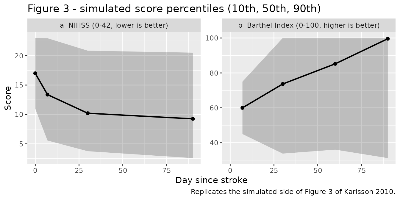
Figure 4 – simulated change from baseline
cfb <- function(traj, scale_label) {
  base <- traj |>
    dplyr::filter(day == min(day)) |>
    dplyr::select(id, base_score = score)
  traj |>
    dplyr::inner_join(base, by = "id") |>
    dplyr::filter(!is.na(score), day > min(day)) |>
    dplyr::mutate(delta = score - base_score) |>
    dplyr::group_by(day) |>
    dplyr::summarise(
      Q10 = quantile(delta, 0.10),
      Q50 = quantile(delta, 0.50),
      Q90 = quantile(delta, 0.90),
      .groups = "drop"
    ) |>
    dplyr::mutate(scale = scale_label)
}

fig4 <- dplyr::bind_rows(
  cfb(traj_nihss, "a  NIHSS change from admission"),
  cfb(traj_bi,    "b  Barthel Index change from day 7")
)

ggplot(fig4, aes(day, Q50)) +
  geom_ribbon(aes(ymin = Q10, ymax = Q90), alpha = 0.25) +
  geom_line(linewidth = 0.8) +
  geom_point(size = 1.6) +
  geom_hline(yintercept = 0, linetype = "dashed", colour = "grey40") +
  facet_wrap(~scale, scales = "free_y") +
  labs(x = "Day since stroke", y = "Change from baseline score",
       title = "Figure 4 - simulated change from baseline (10th, 50th, 90th percentiles)",
       caption = "Replicates the simulated side of Figure 4 of Karlsson 2010.")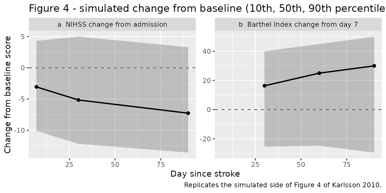
Transition-event mix and informative dropout
The feature that distinguishes this model class from a conventional longitudinal analysis is that dropout is modelled rather than discarded, and is driven by the predicted score. The panel below shows the event mix per visit and the dependence of the dropout probability on the predicted declined score.
event_mix <- dplyr::bind_rows(
  traj_nihss |> dplyr::filter(event != "start") |> dplyr::mutate(scale = "NIHSS"),
  traj_bi    |> dplyr::filter(event != "start") |> dplyr::mutate(scale = "Barthel Index")
) |>
  dplyr::count(scale, day, event) |>
  dplyr::group_by(scale, day) |>
  dplyr::mutate(fraction = n / sum(n)) |>
  dplyr::ungroup()

ggplot(event_mix, aes(factor(day), fraction, fill = event)) +
  geom_col() +
  facet_wrap(~scale) +
  labs(x = "Day since stroke", y = "Fraction of subjects", fill = NULL,
       title = "Transition-event mix at each visit")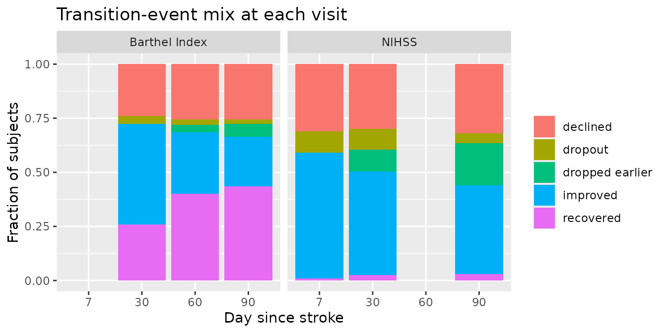
# Deterministic covariate sweeps at typical values -- one row per grid point,
# not per simulated participant.
grid_n <- solve_nihss(seq(0, 42, length.out = 100))
#> Warning: some etas defaulted to non-mu referenced, possible parsing error: etalogitimpr_dlt14, etalogitimpr_dge14, etalogitdecl_dlt14, etalogitdecl_dge14
#> as a work-around try putting the mu-referenced expression on a simple line
#> Warning: multi-subject simulation without without 'omega'
grid_b <- solve_bi(seq(0, 100, length.out = 100))
#> Warning: multi-subject simulation without without 'omega'

dplyr::bind_rows(
  tibble::tibble(scale = "NIHSS (0-42)",
                 predicted = grid_n$nihss_decline, p_dropout = grid_n$p_dropout),
  tibble::tibble(scale = "Barthel Index (0-100)",
                 predicted = grid_b$bi_decline,    p_dropout = grid_b$p_dropout)
) |>
  ggplot(aes(predicted, p_dropout)) +
  geom_line(linewidth = 0.8) +
  facet_wrap(~scale, scales = "free_x") +
  labs(x = "Model-predicted declined score", y = "p(dropout)",
       title = "Informative dropout: p(dropout) against the predicted declined score",
       subtitle = "Typical values, day 30. Opposite slopes because the scales run in opposite directions.")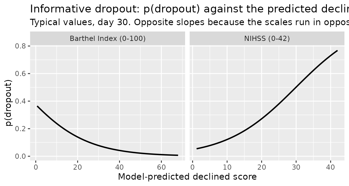
Validation
This paper has no PK layer, no dose and no concentration, so NCA is not the applicable check. The gates below are the structural and behavioural ones the model class admits.
score_range <- function(traj) range(traj$score, na.rm = TRUE)
r_nihss <- score_range(traj_nihss)
r_bi    <- score_range(traj_bi)

# Median score at the day-90 endpoint versus baseline.
med_at <- function(traj, d) median(traj$score[traj$day == d], na.rm = TRUE)
nihss_base <- med_at(traj_nihss, 0)
nihss_d90  <- med_at(traj_nihss, 90)
bi_base    <- med_at(traj_bi, 7)
bi_d90     <- med_at(traj_bi, 90)

# Fraction still in study at day 90.
retained <- function(traj) mean(!traj$dropped[traj$day == max(traj$day)])
ret_nihss <- retained(traj_nihss)
ret_bi    <- retained(traj_bi)

checks <- tibble::tribble(
  ~Check, ~Value, ~Requirement,
  "NIHSS scores stay within [0, 43]",
    sprintf("[%.2f, %.2f]", r_nihss[1], r_nihss[2]), "the 0-42 scale plus the source's +1 offset",
  "Barthel Index scores stay within [0, 101]",
    sprintf("[%.2f, %.2f]", r_bi[1], r_bi[2]),       "the 0-100 scale plus the source's +1 offset",
  "Median NIHSS improves from admission to day 90",
    sprintf("%.1f -> %.1f", nihss_base, nihss_d90),  "lower is better",
  "Median Barthel Index improves from day 7 to day 90",
    sprintf("%.1f -> %.1f", bi_base, bi_d90),        "higher is better",
  "Fraction retained at day 90 (NIHSS model)",
    sprintf("%.2f", ret_nihss),                      "between 0.50 and 0.95",
  "Fraction retained at day 90 (BI model)",
    sprintf("%.2f", ret_bi),                         "between 0.60 and 0.99"
)

knitr::kable(checks, caption = "Structural and behavioural validation of the packaged models.")| Check | Value | Requirement |
|---|---|---|
| NIHSS scores stay within [0, 43] | [0.00, 39.38] | the 0-42 scale plus the source’s +1 offset |
| Barthel Index scores stay within [0, 101] | [2.58, 100.48] | the 0-100 scale plus the source’s +1 offset |
| Median NIHSS improves from admission to day 90 | 17.0 -> 9.3 | lower is better |
| Median Barthel Index improves from day 7 to day 90 | 60.0 -> 99.6 | higher is better |
| Fraction retained at day 90 (NIHSS model) | 0.76 | between 0.50 and 0.95 |
| Fraction retained at day 90 (BI model) | 0.92 | between 0.60 and 0.99 |
stopifnot(
  # Bounds are a hard property of the reconstruction rules, not a cohort draw.
  # The +1 upper slack is the source's own offset: an "improvement" from
  # SCORE_NIHSS_PREV can land at SCORE_NIHSS_PREV + 1 when imz is near 0, and a
  # "decline" from a maximal Barthel Index can land at 101 when dez is near 0.
  r_nihss[1] >= 0, r_nihss[2] <= 43,
  r_bi[1]    >= 0, r_bi[2]    <= 101,

  # Direction and magnitude of the population trend at the endpoint. Asserted
  # as a trend with headroom rather than as a step-by-step ordering, because
  # visit-to-visit medians of a cohort this size can cross. Realised on the
  # authoring run: NIHSS median 17.0 -> 9.3 (a 7.7-point improvement) and BI
  # median 60.0 -> 99.6 (39.6 points). The bounds below sit well inside that
  # and still go red if the improvement and decline reconstruction rules are
  # swapped, which would send both trends the other way.
  nihss_base - nihss_d90 > 2,
  bi_d90 - bi_base       > 10,

  # Retention at day 90. This is the gate on the informative-dropout sign: with
  # slope_score_p_dropout flipped, the NIHSS model drops essentially nobody
  # (retention -> 1.0) and the BI model drops most of the cohort. Realised on
  # the authoring run: 0.76 (NIHSS) and 0.92 (BI); binomial standard errors at
  # n = 200 are 0.03 and 0.02, so both bounds carry several standard errors of
  # headroom in each direction.
  ret_nihss > 0.50, ret_nihss < 0.95,
  ret_bi    > 0.60, ret_bi    < 0.99
)
A note on the bounds check: the + 1 slack is not a
tolerance, it is the source’s convention. Karlsson 2010’s Table I treats
an unchanged score as a decline, and the reconstruction rules carry a
+ 1 offset
((1 - imz) * (SCORE_NIHSS_PREV + 1),
(1 - dez) * (SCORE_BI_PREV + 1)) so that a full improvement
can reach the scale endpoint exactly. The cost is that a minimal
improvement can overshoot by up to one point. The packaged models
reproduce that rather than clamping it.
Assumptions and deviations
Parameter provenance
-
Supplement A over Supplement B. Every packaged
value is the final estimate from Supplement A. Supplement B’s
$THETA/$OMEGArecords are NONMEM initial estimates and disagree with Supplement A on several NIHSS parameters and on 11 of 15 BI thetas plus the omega (1.25 vs 2.08). The adjudication is the paper’s own stated NIHSS age effect, reproduced under Supplement A and not under Supplement B; see the Source trace section. - BI age effect (claim 3) is a recorded deviation, reproducing as 0.0795 against a published 0.07. Not tuned.
Corrections to the source supplements
-
TLSis mislabelled in the Supplement B dataset legend. The legend reads “TLS = Time since start of study (i.e. time since stroke) in days”. The tabulated data falsify it: in the NIHSS excerpt subject 2 hasDAY 8 -> TLS 7,DAY 33 -> TLS 25(= 33 - 8),DAY 62 -> TLS 29(= 62 - 33); in the BI excerptTLSis non-monotonic inDAY, which a time-since-stroke clock cannot be.TLSis time since the previous observation and is packaged asT_PREVOBS. Table II corroborates this by listing “Influence of time since previous observation” and “Influence of time since baseline” as separate rows; the second clock isTSS = DAY, carried here by rxode2’stime. Taking the legend at face value would silently mis-specifye_t_prevobs_p_notmax(NIHSS) ande_t_prevobs_decl(BI). -
Four undefined variables in the BI control stream are
omitted. That stream writes
DECOV = DETLS + DEGGT + DEANG,A1COV = A1PBI + A1AGE + A1CGLandA2COV = A2PBI + A2TLS + A2TSS, butDEGGT,DEANG,A1CGLandA2TLSare never assigned anywhere in it – vestigial covariate-screening terms, with GGT, ANG and CGL surviving undropped in the BI$INPUT. None has a counterpart among Supplement A’s 15 BI thetas or in Table II, so all four are zero in the final model and are omitted from the packaged file. -
The BI
$THETA(1)inline comment is wrong. It reads “Probability of decline (logit scale)”, but the code assignsP1A = P1 ; Improvement, Supplement A names the parameterPrIM, and the covariate signs match improvement. The code and the paper agree; the comment does not. -
No IIV on the BI improvement magnitude, despite the
Results prose. Karlsson 2010 states the BI relative-improvement model
included “terms for interindividual variability and residual
variability”, but the Supplement B stream has
IM = TVIM + RVwith noETAterm whileDE = TVDE + ETA(1) + RV, and Supplement A lists a single omega labelled “IIV on decline”. The equation governs. -
AGE = -99missing-value branching is not reproduced. The BI stream branches onIF(AGE.EQ.-99)to zero both age effects. That is a NONMEM data-coding convention, not model structure; supply a real age.
Encoding
-
Placeholder residuals on the three probability
endpoints. The source likelihood for
p_improve,p_notmaxandp_dropoutis Bernoulli on the observed binary event (NONMEMF_FLAG = 1), which carries no residual-error parameter. rxode2 requires an error model per endpoint, so each probability is emitted with a fixed additive residual SD of 0.001, followingFukae_2024_valemetostat_orr_investigator. Do not read these as estimates. -
addSd_imzandaddSd_dezare one source parameter written twice. The source declares$SIGMA 1 FIXwithRV = THETA(6)*EPS(1)and applies that single term to both the improvement and the decline function. rxode2 requires a distinct endpoint parameter per endpoint. -
The etas are not mu-referenced. Which eta applies
switches with time in the NIHSS model, so the eta cannot sit on a simple
theta + etaline. rxode2 warns about this at parse time; it is correct for this model and affects simulation not at all.
Simulation choices in this vignette
- Covariate dispersions are assumed. The paper reports means and ranges but no standard deviations. Age is drawn N(71.7, 12) truncated to 26-90 and baseline NIHSS N(16.8, 5) truncated to 4-31, so that the simulated means and ranges match the published ones.
- The day-7 Barthel Index seed is constructed, not published. The BI has no admission assessment and the paper reports no day-7 BI distribution, so each subject’s starting BI is mapped from their baseline NIHSS on the reversed scale and rounded to the scale’s five-point grid. This is a starting condition for the demonstration only; it is not a model parameter and nothing in the packaged model depends on it.
-
T_PREVOBSat the first NIHSS transition is taken as 7 days (admission at day 0). The source dataset implies an admission assessment on day 1 (DAY 7 -> TLS 6), a one-day difference with no material effect. - The recursion draws Bernoulli events and logit-scale residuals in R. The packaged models supply every probability, every logit-scale prediction and both reconstruction rules; only the random draws and the carry-forward of the previous score happen in the vignette. This is the same walk the authors used to generate their 10,000-subject diagnostic simulation, at the 200-subject scale this package caps cohorts at.