SLE latent-variable MBMA (Goteti 2024)
Source:vignettes/articles/Goteti_2024_SLE_mbma.Rmd
Goteti_2024_SLE_mbma.RmdModel and source
- Citation: Goteti K, Garcia R, Gillespie WR, French J, Klopp-Schulze L, Li Y, Vazquez Mateo C, Roy S, Guenther O, Benincosa L, Venkatakrishnan K. Model-based meta-analysis using latent variable modeling to set benchmarks for new treatments of systemic lupus erythematosus. CPT Pharmacometrics Syst Pharmacol. 2024;13(2):281-295. doi:10.1002/psp4.13083.
- Description: MBMA. Bayesian latent-variable disease-trajectory model-based meta-analysis (DTM-MBMA) of composite systemic lupus erythematosus (SLE) endpoints across 25 studies, 81 study arms, and 16 SLE treatments (Goteti 2024 Table 1). A uni-dimensional latent SLE disease activity theta(t) is modelled as a mono-exponential approach from a baseline mu_ijk to a long-term level mu_ijk + delta_ijk with time-constant log(2)/lam (Goteti 2024 Eq 1). The paper reparametrizes mu and delta in terms of the more-observable theta_wk4 (latent SLE at week 4) and delta_wk24 (increment from week 4 to week 24), separately for the SRI (SRI-4/5/6) and BICLA endpoints. Mean baseline SLEDAI (centered at 10.5) modifies both mu (via beta_sledai_mu) and delta (via beta_sledai_delta). Continuous-dose Emax dose-response was fit for six drugs whose regimen had three or more doses at the same route and frequency: anifrolumab (i.v. q4w), belimumab (i.v. q2wx3+q4w), CC-220 (oral qd), epratuzumab (i.v. q2w), lulizumab pegol (s.c. q2w), and sifalimumab (i.v. q2w). All 24 other drug-dose-regimen combinations from Table 4 (ALX-0061, atacicept, baricitinib, the s.c. q.w. belimumab arm, the i.v. q.w. epratuzumab arm, evobrutinib, fenebrutinib, IPP-201101, the s.c. q.w. lulizumab pegol arm, lupuzor, PF-04236921, tabalumab, ustekinumab) were modelled as discrete per-regimen additive effects on the latent-scale delta multiplier (1 + xi_ij); the user passes the reference discrete-effect value through the CONMED_XI_DISCRETE covariate (documented lookup in the vignette). SRI-4/5/6 responder probabilities are modelled as a generalized proportional-odds transform of the latent SLE activity (thresholds c_SRI5 = 0.586, c_SRI6 = 0.693), and BICLA responder probability is the logistic transform of the latent SLE activity directly. Between-study variability is encoded as study-level etas on theta_wk4 and delta_wk24 for both endpoints (no subject-level IIV); the simulation scope is aggregate study-arm-mean responder probability, not individual patient trajectories. All Table 3 point estimates are the posterior mean under the reference Bayesian fit (model 106-bm-1 in Table S1 of the supplement).
- Article: https://doi.org/10.1002/psp4.13083 (Open Access)
- Supplement: available with the article; contains the disease-trajectory reparametrization (Eq 3-5), the study-effect Eq 6-7, the generalized proportional-odds SRI observation model, and the missing-baseline-SLEDAI data model.
Population
Goteti 2024 built a Bayesian model-based meta-analysis (MBMA) of composite Systemic Lupus Erythematosus (SLE) endpoints across 25 randomized clinical trials, 81 treatment arms, and 16 SLE therapeutics (Table 1). All 25 studies included a placebo + standard of care (SoC) comparator arm; placebo + SoC arms for studies that were not identified in the literature review were collected through the TransCelerate BioPharma Historical Trial Data Sharing Initiative. The dataset totalled approximately 12,136 patients (Table 1 sample-size column sum) with an across-arm mean age of 40.2 years (per-arm mean range 31.7-46.4 years, Table 2), 94.1% female (range 83.3-100%), and a race distribution of 64.4% White, 13.6% Asian, 11.2% Black, and 14.9% other (Table 2 across-arm means). Regional distribution across arms that reported region was 34.2% North America, 19.5% Central/South America, 17.5% Asia, and 27.0% other (Table 2). Baseline SLE severity, measured by the mean Systemic Lupus Erythematosus Disease Activity Index (SLEDAI), was 10.5 across arms (range 8.8-14.0 across the 75% of arms that reported it); this across-arm mean of 10.5 is the centring point for the SLEDAI covariate in the MBMA model.
The MBMA operates at the study-arm level: each modelled observation is the aggregate response rate (SRI-4/5/6 or BICLA) in one arm at one visit time, with the arm’s total sample size used as the binomial / multinomial denominator in the joint likelihood (supplement Eq 11-13). Simulations from this model produce study-arm-mean responder probabilities and are not suitable for individual-subject simulation.
The same metadata is available programmatically via
readModelDb("Goteti_2024_SLE_mbma")()$population.
Source trace
The per-parameter origin is recorded as an in-file comment next to
each ini() entry in
inst/modeldb/therapeuticArea/Goteti_2024_SLE_mbma.R. The
table below collects them in one place for review.
| Equation / parameter | Value (as encoded) | Source location |
|---|---|---|
theta_wk4_SRI |
logit(0.170) = -1.587 |
Goteti 2024 Table 3 (probability-scale 0.170) |
delta_wk24_SRI |
logit(0.469) - logit(0.170) = +1.463 |
Table 3 (probability-scale wk-24 value 0.469 for
theta_wk4 + delta_wk24) |
theta_wk4_BICLA |
logit(0.247) = -1.115 |
Table 3 (probability-scale 0.247) |
delta_wk24_BICLA |
logit(0.412) - logit(0.247) = +0.760 |
Table 3 (probability-scale wk-24 value 0.412 for
theta_wk4 + delta_wk24) |
lthalf (t_1/2) |
log(4.51) = 1.506 | Table 3 (t_1/2 = 4.51 wk) |
c_SRI5 |
0.586 | Table 3 c_2,SRI |
c_SRI6 |
0.693 | Table 3 c_3,SRI |
beta_sledai_mu |
0.208 | Table 3 beta_SLEDAI,0 |
beta_sledai_delta |
0.255 | Table 3 beta_SLEDAI,delta |
Emax_ANIF |
0.257 | Table 4 (anifrolumab i.v. q4w) |
ED50_ANIF |
259 mg | Table 4 |
Emax_BEL |
0.165 | Table 4 (belimumab i.v. q2wx3+q4w) |
ED50_BEL |
0.787 mg/kg | Table 4 |
Emax_CC220 |
0.415 | Table 4 (CC-220 oral qd) |
ED50_CC220 |
0.415 mg | Table 4 |
Emax_EPRA |
0.397 | Table 4 (epratuzumab i.v. q2w) |
ED50_EPRA |
827 mg | Table 4 |
Emax_LULI |
0.165 | Table 4 (lulizumab pegol s.c. q2w) |
ED50_LULI |
9.47 mg | Table 4 |
Emax_SIFA |
0.0131 | Table 4 (sifalimumab i.v. q2wx3+q4w) |
ED50_SIFA |
942 mg | Table 4 |
| study eta variances | see model file | Table 3 sigma_4w,k and sigma_delta,k (variance = sigma^2) |
| DTM ODE / algebra | n/a | Goteti 2024 Eq 1 + supplement Eq 3-8 |
| Proportional-odds SRI | n/a | Supplement Section 1.3 “Model for SRI” |
| Logit BICLA | n/a | Supplement Section 1.3 “Model for BICLA” |
Model structure summary
Latent SLE disease activity theta(t) evolves
mono-exponentially from a baseline mu to a long-term level
mu + delta (Eq 1):
The paper reparametrizes (mu, delta) in terms of
(theta_wk4, delta_wk24) because the summary-level data are
concentrated at weeks 4 and 24 (supplement Eq 3, 5):
Baseline SLEDAI (centred at 10.5) and drug effect xi_ij
enter multiplicatively on the latent scale (Eq 8):
Responder probabilities:
- BICLA:
p_BICLA(t) = expit(theta_BICLA(t)). - SRI-4/5/6: generalized proportional-odds transform with thresholds
c_0 = 0, c_SRI5, c_SRI6(larger threshold = stricter response),p_SRI-l(t) = expit(theta_SRI(t) - c_l).
Continuous-Emax drugs (six regimens with three-plus doses at the same
route and frequency):
xi_d = (Dose * Emax_d) / (Dose + ED50_d). The other 24
drug-dose-regimen combinations use discrete per-arm effects passed
through the CONMED_XI_DISCRETE covariate; the lookup values
are listed in the model file’s covariateData notes.
Virtual cohort
MBMA operates at the study-arm level, so a “cohort” here is a set of study-arm scenarios (drug/regimen combinations at fixed baseline SLEDAI), each simulated at the same time grid.
The vignette below stays well under the 200-per-arm cap by simulating
one subject per scenario (the model has no per-subject stochasticity at
the individual level; between-study variability is applied via the four
study etas, and typical-value predictions use
rxode2::zeroRe()).
mod_full <- readModelDb("Goteti_2024_SLE_mbma")
mod_typ  <- rxode2::zeroRe(mod_full)

# Standard MBMA-scenario builder: one row per scenario. All non-active drug
# doses / indicators are zero for arms whose drug is covered by a different
# column (only one drug per arm in the source paper).
make_scenarios <- function(scenarios, times, id_offset = 0L) {
  scn <- scenarios |> mutate(id = id_offset + row_number())
  base <- expand.grid(
    id = scn$id,
    time = times,
    KEEP.OUT.ATTRS = FALSE,
    stringsAsFactors = FALSE
  )
  base$amt  <- 0
  base$evid <- 0L
  base$cmt  <- NA_character_  # algebraic model; no ODE state
  base <- dplyr::left_join(base, scn, by = "id")
  # Fill any missing covariate columns with 0 so the model always sees them.
  need <- c(
    "SCORE_SLEDAI", "DOSE_ANIFROLUMAB_MG", "DOSE_BELIMUMAB_MGKG",
    "DOSE_CC220_MG", "DOSE_EPRATUZUMAB_IVQ2W_MG",
    "DOSE_LULIZUMAB_SCQ2W_MG", "DOSE_SIFALIMUMAB_MG", "CONMED_XI_DISCRETE"
  )
  for (nm in need) {
    if (!nm %in% names(base)) base[[nm]] <- 0
  }
  base
}
Placebo response – Table 3 recapitulation
Goteti 2024 Table 3 reports that a placebo + SoC arm with mean baseline SLEDAI = 10.5 has an SRI-4 response probability of 0.170 at week 4 and 0.469 at week 24, and a BICLA response probability of 0.247 at week 4 and 0.412 at week 24. The typical-value simulation below should recover these values (differences at the second decimal are within reported credible interval widths).
placebo <- data.frame(
  scenario = "Placebo + SoC (SLEDAI 10.5)",
  SCORE_SLEDAI = 10.5,
  CONMED_XI_DISCRETE = 0
)

ev_placebo <- make_scenarios(placebo, times = c(0, 2, 4, 8, 12, 16, 24, 36, 52))

sim_placebo <- rxode2::rxSolve(mod_typ, events = ev_placebo,
                               keep = c("scenario")) |>
  as.data.frame()
#> ℹ omega/sigma items treated as zero: 'eta_wk4_SRI', 'eta_delta_SRI', 'eta_wk4_BICLA', 'eta_delta_BICLA'

wk4_wk24 <- sim_placebo |>
  filter(time %in% c(4, 24)) |>
  select(scenario, time, p_SRI4, p_SRI5, p_SRI6, p_BICLA)

wk4_wk24 |>
  dplyr::rename(
    "Scenario"          = scenario,
    "Time (wk)"         = time,
    "p(SRI-4)"          = p_SRI4,
    "p(SRI-5)"          = p_SRI5,
    "p(SRI-6)"          = p_SRI6,
    "p(BICLA)"          = p_BICLA
  ) |>
knitr::kable(digits = 3, caption = "Placebo + SoC response probabilities at week 4 and 24; compare Goteti 2024 Table 3 (p_SRI-4 = 0.170 at wk 4 and 0.469 at wk 24; p_BICLA = 0.247 at wk 4 and 0.412 at wk 24).")| Scenario | Time (wk) | p(SRI-4) | p(SRI-5) | p(SRI-6) | p(BICLA) |
|---|---|---|---|---|---|
| Placebo + SoC (SLEDAI 10.5) | 4 | 0.170 | 0.102 | 0.093 | 0.247 |
| Placebo + SoC (SLEDAI 10.5) | 24 | 0.469 | 0.330 | 0.306 | 0.412 |
sim_placebo |>
  select(time, p_SRI4, p_SRI5, p_SRI6, p_BICLA) |>
  pivot_longer(-time, names_to = "endpoint", values_to = "p") |>
  ggplot(aes(x = time, y = p, colour = endpoint)) +
  geom_line(linewidth = 1) +
  geom_point(size = 1.6) +
  scale_y_continuous(limits = c(0, 0.6), labels = scales::percent_format(1)) +
  labs(x = "Time (weeks)", y = "Responder probability",
       colour = NULL,
       title = "Placebo + SoC responder probability over time",
       caption = "Simulated typical-value response for placebo + SoC at baseline SLEDAI = 10.5.") +
  theme_bw() +
  theme(legend.position = "top")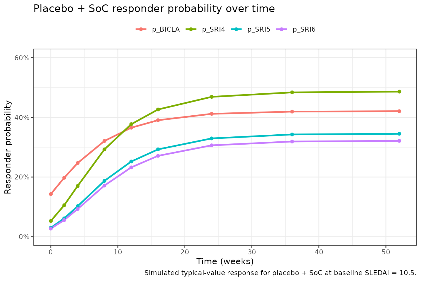
Placebo + SoC response probability over time at baseline SLEDAI = 10.5 (typical value).
Anifrolumab dose-response – Table 4 recapitulation
Goteti 2024 reports that the FDA-approved anifrolumab i.v. 300 mg q4w dose achieves an SRI-4 response of 58% and a BICLA response of 47% at 1 year (Results, second-to-last paragraph before Figure 2). At the model’s ED50 of 259 mg the drug effect achieves half of its Emax.
anif_doses <- data.frame(
  scenario           = paste0("ANIF_", c(0, 50, 100, 150, 200, 259, 300, 500, 750, 1000, 1500, 2000)),
  DOSE_ANIFROLUMAB_MG = c(0, 50, 100, 150, 200, 259, 300, 500, 750, 1000, 1500, 2000),
  SCORE_SLEDAI        = 10.5,
  CONMED_XI_DISCRETE  = 0
)

ev_anif <- make_scenarios(anif_doses, times = 52)
sim_anif <- rxode2::rxSolve(mod_typ, events = ev_anif,
                            keep = c("scenario", "DOSE_ANIFROLUMAB_MG")) |>
  as.data.frame() |>
  filter(time == 52)
#> ℹ omega/sigma items treated as zero: 'eta_wk4_SRI', 'eta_delta_SRI', 'eta_wk4_BICLA', 'eta_delta_BICLA'
#> Warning: multi-subject simulation without without 'omega'

ggplot(sim_anif, aes(x = DOSE_ANIFROLUMAB_MG)) +
  geom_line(aes(y = p_SRI4, colour = "SRI-4"), linewidth = 1) +
  geom_line(aes(y = p_BICLA, colour = "BICLA"), linewidth = 1) +
  geom_vline(xintercept = 259, linetype = "dashed", alpha = 0.5) +
  geom_vline(xintercept = 300, linetype = "dotted", alpha = 0.7) +
  scale_y_continuous(limits = c(0, 0.8), labels = scales::percent_format(1)) +
  labs(x = "Anifrolumab dose (mg IV q4w)",
       y = "Responder probability at week 52",
       colour = NULL,
       title = "Anifrolumab dose-response at 1 year (SLEDAI 10.5)",
       caption = "Dashed line: ED50 = 259 mg (Table 4). Dotted line: FDA-approved 300 mg dose.") +
  theme_bw() +
  theme(legend.position = "top")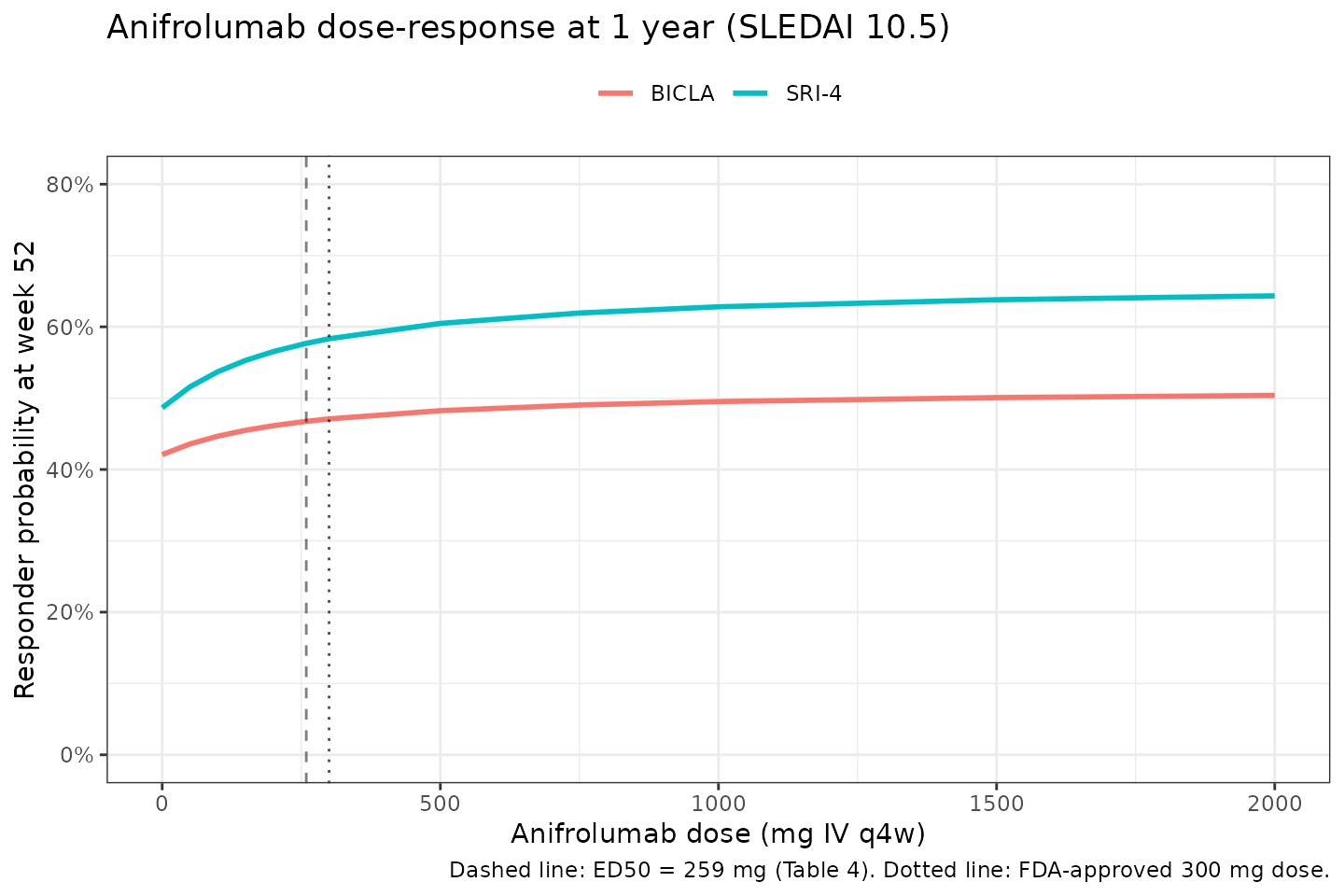
Anifrolumab i.v. q4w dose-response for SRI-4 and BICLA at 1 year (52 weeks), reproducing the Emax dose-response tabulated in Goteti 2024 Table 4.
sim_anif |>
  filter(DOSE_ANIFROLUMAB_MG %in% c(0, 150, 259, 300, 1000)) |>
  transmute(
    Dose         = DOSE_ANIFROLUMAB_MG,
    p_SRI4       = p_SRI4,
    p_BICLA      = p_BICLA
  ) |>
  dplyr::rename(
    "Anifrolumab dose (mg IV q4w)" = Dose,
    "p(SRI-4) at wk 52"            = p_SRI4,
    "p(BICLA) at wk 52"            = p_BICLA
  ) |>
knitr::kable(digits = 3, caption = "Anifrolumab response probability at 1 year (typical placebo + SoC background, SLEDAI = 10.5). Compare Goteti 2024 Results narrative: 300 mg i.v. q4w = 58% SRI-4 and 47% BICLA at 1 year.")| Anifrolumab dose (mg IV q4w) | p(SRI-4) at wk 52 | p(BICLA) at wk 52 |
|---|---|---|
| 0 | 0.486 | 0.421 |
| 150 | 0.553 | 0.455 |
| 259 | 0.577 | 0.467 |
| 300 | 0.583 | 0.471 |
| 1000 | 0.628 | 0.495 |
Belimumab dose-response – Table 4 recapitulation
Goteti 2024 reports that the FDA-approved belimumab i.v. 10 mg/kg q2wx3+q4w dose achieves an SRI-4 response of 59% and a BICLA response of 48% at 1 year (Results, before Figure 2). At the model’s ED50 of 0.787 mg/kg the drug effect achieves half of its Emax.
bel_doses <- data.frame(
  scenario            = paste0("BEL_", c(0, 0.25, 0.5, 0.787, 1, 2, 4, 10, 20)),
  DOSE_BELIMUMAB_MGKG = c(0, 0.25, 0.5, 0.787, 1, 2, 4, 10, 20),
  SCORE_SLEDAI        = 10.5,
  CONMED_XI_DISCRETE  = 0
)

ev_bel <- make_scenarios(bel_doses, times = 52)
sim_bel <- rxode2::rxSolve(mod_typ, events = ev_bel,
                           keep = c("scenario", "DOSE_BELIMUMAB_MGKG")) |>
  as.data.frame() |>
  filter(time == 52)
#> ℹ omega/sigma items treated as zero: 'eta_wk4_SRI', 'eta_delta_SRI', 'eta_wk4_BICLA', 'eta_delta_BICLA'
#> Warning: multi-subject simulation without without 'omega'

ggplot(sim_bel, aes(x = DOSE_BELIMUMAB_MGKG)) +
  geom_line(aes(y = p_SRI4, colour = "SRI-4"), linewidth = 1) +
  geom_line(aes(y = p_BICLA, colour = "BICLA"), linewidth = 1) +
  geom_vline(xintercept = 0.787, linetype = "dashed", alpha = 0.5) +
  geom_vline(xintercept = 10, linetype = "dotted", alpha = 0.7) +
  scale_x_log10() +
  scale_y_continuous(limits = c(0, 0.8), labels = scales::percent_format(1)) +
  labs(x = "Belimumab dose (mg/kg IV q2wx3+q4w, log scale)",
       y = "Responder probability at week 52",
       colour = NULL,
       title = "Belimumab dose-response at 1 year (SLEDAI 10.5)",
       caption = "Dashed line: ED50 = 0.787 mg/kg (Table 4). Dotted line: FDA-approved 10 mg/kg dose.") +
  theme_bw() +
  theme(legend.position = "top")
#> Warning in scale_x_log10(): log-10 transformation introduced infinite values.
#> Warning in scale_x_log10(): log-10 transformation introduced infinite values.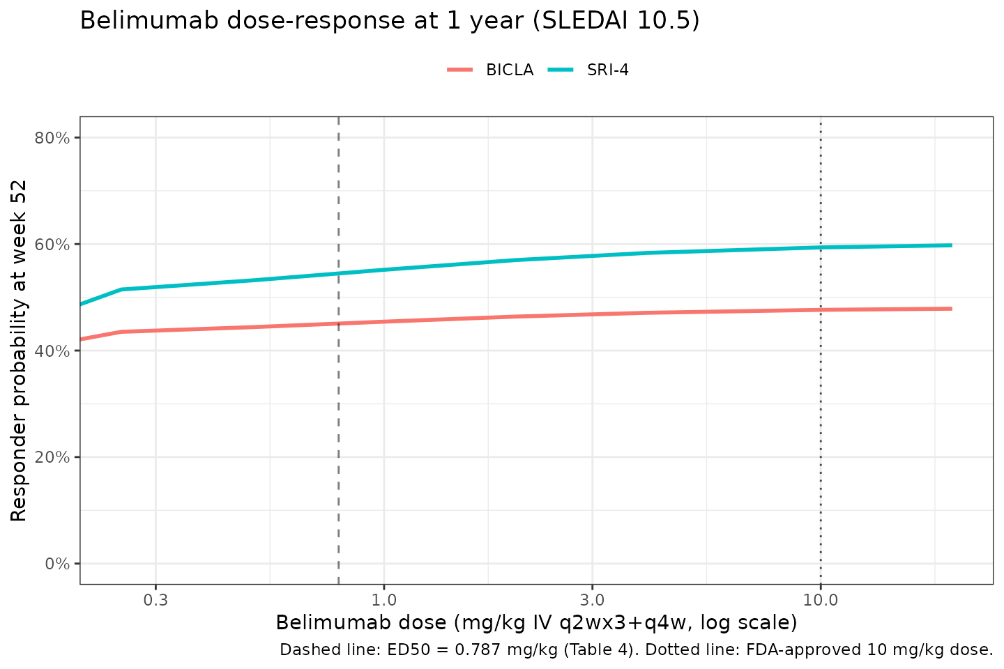
Belimumab i.v. q2wx3+q4w dose-response for SRI-4 and BICLA at 1 year (52 weeks).
sim_bel |>
  filter(DOSE_BELIMUMAB_MGKG %in% c(0, 0.787, 1, 4, 10)) |>
  transmute(
    Dose    = DOSE_BELIMUMAB_MGKG,
    p_SRI4  = p_SRI4,
    p_BICLA = p_BICLA
  ) |>
  dplyr::rename(
    "Belimumab dose (mg/kg IV q2wx3+q4w)" = Dose,
    "p(SRI-4) at wk 52"                    = p_SRI4,
    "p(BICLA) at wk 52"                    = p_BICLA
  ) |>
knitr::kable(digits = 3, caption = "Belimumab response probability at 1 year (typical placebo + SoC background, SLEDAI = 10.5). Compare Goteti 2024 Results: 10 mg/kg i.v. q2wx3+q4w = 59% SRI-4 and 48% BICLA at 1 year.")| Belimumab dose (mg/kg IV q2wx3+q4w) | p(SRI-4) at wk 52 | p(BICLA) at wk 52 |
|---|---|---|
| 0.000 | 0.486 | 0.421 |
| 0.787 | 0.545 | 0.451 |
| 1.000 | 0.552 | 0.454 |
| 4.000 | 0.583 | 0.471 |
| 10.000 | 0.594 | 0.476 |
Baseline SLEDAI covariate effect
Higher baseline SLEDAI increases both baseline latent activity (via
beta_sledai_mu = 0.208) and long-term latent change (via
beta_sledai_delta = 0.255), so higher-severity cohorts show
larger placebo response probabilities.
sledai_grid <- data.frame(
  scenario           = paste0("SLEDAI_", seq(8, 14, by = 1)),
  SCORE_SLEDAI       = seq(8, 14, by = 1),
  CONMED_XI_DISCRETE = 0
)

ev_sledai <- make_scenarios(sledai_grid, times = 52)
sim_sledai <- rxode2::rxSolve(mod_typ, events = ev_sledai,
                              keep = c("scenario", "SCORE_SLEDAI")) |>
  as.data.frame() |>
  filter(time == 52)
#> ℹ omega/sigma items treated as zero: 'eta_wk4_SRI', 'eta_delta_SRI', 'eta_wk4_BICLA', 'eta_delta_BICLA'
#> Warning: multi-subject simulation without without 'omega'

sim_sledai |>
  select(SCORE_SLEDAI, p_SRI4, p_BICLA) |>
  pivot_longer(-SCORE_SLEDAI, names_to = "endpoint", values_to = "p") |>
  ggplot(aes(x = SCORE_SLEDAI, y = p, colour = endpoint)) +
  geom_line(linewidth = 1) +
  geom_point(size = 1.6) +
  scale_y_continuous(limits = c(0, 0.6), labels = scales::percent_format(1)) +
  labs(x = "Baseline SLEDAI (per-arm mean)",
       y = "Responder probability at week 52",
       colour = NULL,
       title = "Placebo + SoC response at 1 year across baseline SLEDAI",
       caption = "Baseline SLEDAI covariate effect on placebo + SoC (SLEDAI centered at 10.5).") +
  theme_bw() +
  theme(legend.position = "top")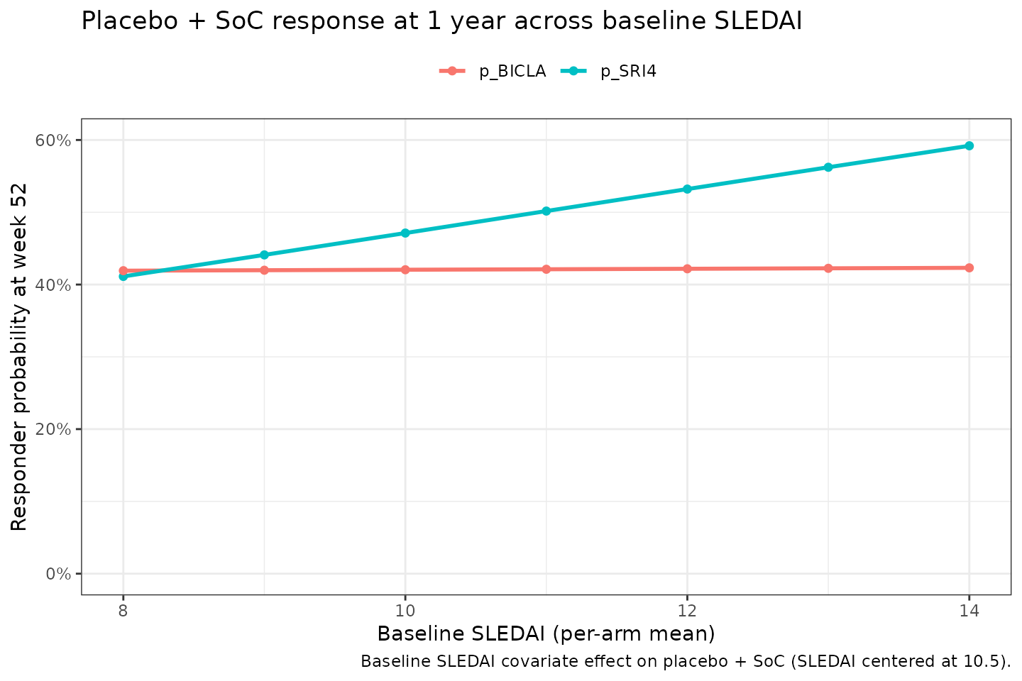
Placebo + SoC SRI-4 response probability at 1 year across baseline-SLEDAI values from 8 to 14 (covering the observed across-arm range in Goteti 2024 Table 2).
Discrete-effect regimens – Table 4 recapitulation
For drug-dose-regimen combinations that did not have three-plus doses
at the same route and frequency, the paper fit per-regimen discrete
effects xi_d on the latent-scale delta multiplier (Table
4). Reproduce a selection of them by passing the tabulated
xi values through the CONMED_XI_DISCRETE
covariate.
discrete_arms <- tibble::tribble(
  ~scenario,                            ~CONMED_XI_DISCRETE,
  "Placebo + SoC",                       0.00,
  "Belimumab 200 mg s.c. q.w.",         +0.16,
  "Epratuzumab 600 mg i.v. q.w.",       +0.324,
  "Tabalumab 120 mg s.c. q2w",          +0.0699,
  "Baricitinib 4 mg oral q.d.",         +0.24,
  "Ustekinumab 6 mg/kg IV + 90 mg SC q8w", -0.182
) |>
  mutate(SCORE_SLEDAI = 10.5)

ev_disc <- make_scenarios(discrete_arms, times = 52)
sim_disc <- rxode2::rxSolve(mod_typ, events = ev_disc,
                            keep = c("scenario", "CONMED_XI_DISCRETE")) |>
  as.data.frame() |>
  filter(time == 52)
#> ℹ omega/sigma items treated as zero: 'eta_wk4_SRI', 'eta_delta_SRI', 'eta_wk4_BICLA', 'eta_delta_BICLA'
#> Warning: multi-subject simulation without without 'omega'

sim_disc |>
  transmute(
    Regimen = scenario,
    xi      = CONMED_XI_DISCRETE,
    p_SRI4  = p_SRI4,
    p_BICLA = p_BICLA
  ) |>
  dplyr::rename(
    "Regimen"           = Regimen,
    "xi (Table 4)"      = xi,
    "p(SRI-4) at wk 52" = p_SRI4,
    "p(BICLA) at wk 52" = p_BICLA
  ) |>
knitr::kable(digits = 3, caption = "Discrete-effect regimen response probabilities at 1 year (typical placebo + SoC background, SLEDAI = 10.5).")| Regimen | xi (Table 4) | p(SRI-4) at wk 52 | p(BICLA) at wk 52 |
|---|---|---|---|
| Placebo + SoC | 0.000 | 0.486 | 0.421 |
| Belimumab 200 mg s.c. q.w. | 0.160 | 0.598 | 0.479 |
| Epratuzumab 600 mg i.v. q.w. | 0.324 | 0.703 | 0.539 |
| Tabalumab 120 mg s.c. q2w | 0.070 | 0.536 | 0.446 |
| Baricitinib 4 mg oral q.d. | 0.240 | 0.651 | 0.508 |
| Ustekinumab 6 mg/kg IV + 90 mg SC q8w | -0.182 | 0.361 | 0.357 |
Assumptions and deviations
Latent-scale storage of Table 3 point estimates. Goteti 2024 Table 3 reports
theta_wk4,kandtheta_wk4,k + delta_wk24,kon the probability scale, but the underlying Bayesian estimation is on the latent (logit) scale on which the SLEDAI / drug / study effects all operate (Eq 8). Theini()entries store the latent-scale values aslog(0.170 / (1 - 0.170))etc., with the probability-scale value documented in each label. Any downstream user who reads the.Rfile sees both scales; there is no re-interpretation.SRI proportional-odds threshold indexing. The supplement writes
p_SRI-l(t) = expit(theta_SRI(t) - c_{l-4})forl = 4, 5, 6withc_0 = 0andc_3 > c_2 > c_1 > c_0. Table 3 reports two thresholds labelledc_2,SRI = 0.586andc_3,SRI = 0.693; the pairing that matches SRI-4 = expit(theta), SRI-5 < SRI-4, SRI-6 < SRI-5 with these two threshold values isc_SRI5 = 0.586(the supplement’sc_1) andc_SRI6 = 0.693(the supplement’sc_2). The apparent supplement / main-text index offset by 1 is a Bayesian-array indexing artefact (Stan arrays are 1-based); the numeric values are unambiguous. Verification at the placebo + SoC typical value: at week 4,p_SRI4 = expit(logit(0.170)) = 0.170(matches Table 3), and the derivedp_SRI5andp_SRI6decrease monotonically as expected.Aggregate-level likelihood not encoded. The paper’s Bayesian likelihood is binomial (BICLA) and multinomial (SRI-4/5/6) at the study-arm level, weighted by per-arm sample size
N_ij(t)(supplement Eq 11-13). nlmixr2 / rxode2 do not natively encode binomial / multinomial residuals for aggregate responder probabilities, so the model exposes the responder probabilities as continuous algebraic outputs (p_SRI4,p_SRI5,p_SRI6,p_BICLA) and attaches a small fixed additive residual placeholder (addSd = 0.001) toCc = p_SRI4to satisfy the nlmixr2 observation-model requirement. Users wanting a full aggregate-level simulation should sampleY_arm ~ Binomial(N_arm, p_arm)post-simulation.Between-study variability encoded as etas. The four study-level random-effect SDs from Table 3 (
sigma_4w,SRI,sigma_delta,SRI,sigma_4w,BICLA,sigma_delta,BICLA) are encoded as independent etas ontheta_wk4_kanddelta_wk24_k. These are BETWEEN-STUDY variances, distinct from popPK between-subject variability. The simulation scope is study-arm-mean responder probability, not individual patient trajectory; this is a fundamental MBMA scope.CONMED_XI_DISCRETE consolidates 24 discrete-effect regimens. Rather than register 24 individual per-regimen indicator covariates, this model passes the appropriate xi value directly. The full lookup lives in
covariateData$CONMED_XI_DISCRETE$notesin the model file and in the discrete-effect scenario table above. When simulating a specific arm, read the arm’s xi from Table 4 and pass it asCONMED_XI_DISCRETE.Lupuzor 200 mg s.c. q4w row printed as “201 mg” in Table 4 – this is interpreted as a Table 4 typo (Table 1 lists Lupuzor at 200 mg for both the q2w and q4w regimens). The 0.205 xi value is used at 200 mg.
Missing-baseline-SLEDAI submodel not encoded. The paper handles arms with missing mean baseline SLEDAI by drawing a per-arm value from a truncated normal
TN(ec_i, mu_SLEDAI, sigma_SLEDAI / sqrt(n_ij))(supplement Eq 10) withmu_SLEDAI = 4.75andsigma_SLEDAI = 5.94(Table 3); this is an estimation-side data-imputation feature and is not part of the forward simulation. If a downstream user has missing arm-level SLEDAI, they should either impute externally (e.g., pass 10.5 as the across-arm mean) or draw from the truncated normal above using the arm’s enrolment criterionec_iand sample sizen_ij.Model reference is 106-bm-1 (relative dose effect on delta, no dose effect on lambda). This is the parsimonious model selected in Goteti 2024 supplement Section 1.5 Table 1 despite marginally worse ELPD than the more complex 107-bm / 108-bm variants; the authors’ rationale (Results, “Consequently, the principle of parsimony was used, and the model with relative dose effect on delta … was selected”) is followed here.