Cardiovascular systems (CVS) QSP model, rat (Fu 2023)
Source:vignettes/articles/Fu_2023_cardiovascular.Rmd
Fu_2023_cardiovascular.RmdModel and source
- Citation: Fu Y, Snelder N, Guo T, van der Graaf PH, van Hasselt JGC. Evaluation of a Cardiovascular Systems Model for Design and Analysis of Hemodynamic Safety Studies. Pharmaceutics. 2023 Apr 7;15(4):1175. doi:10.3390/pharmaceutics15041175. System-specific structure and parameter values inherited from Snelder et al. (2013, 2014); Fu 2023 fixes the system parameters as reported in Supplemental Materials S1 (NONMEM control stream).
- Article: Pharmaceutics 2023, 15(4):1175
- Supplement (NONMEM control stream and Table S1 simulation-scenario matrix): pharmaceutics-2186186-supplementary
The Fu 2023 paper is a stochastic-simulation and re-estimation (SSE) identifiability study of the cardiovascular systems (CVS) QSP model developed by Snelder et al. (J Pharmacokinet Pharmacodyn 2013 40(3):357-373; Br J Pharmacol 2014 171(22):5076-5092) for rat pre-clinical hemodynamic safety studies. The five hemodynamic variables – heart rate (HR), stroke volume (SV), total peripheral resistance (TPR), cardiac output (CO = HR * SV), and mean arterial pressure (MAP = CO * TPR) – are linked through three coupled indirect-response ODEs on HR, SV-turnover (SVT), and TPR, plus a shared MAP-negative-feedback term on the production rate of each state and cosine circadian rhythms on HR and TPR. A hypothetical one-compartment iv-bolus drug with a fixed 4-h half-life perturbs HR-production through an Emax function in the NONMEM code (Fu 2023 Supplemental Materials S1); this vignette reproduces the paper’s baseline hemodynamic behaviour and drug-response magnitudes and demonstrates how the model is used for the SSE identifiability sweep of Section 2.3.
The model is packaged as a QSP model with 4 ODE states
(central, hr, svt,
tpr), 3 algebraic hemodynamic observables (HR,
CO, MAP) plus the drug amount Cc,
12 fixed system-specific parameters (Snelder-derived rat baseline
values, dissipation rate constants, MAP-feedback constant, HR-on-SV
coupling, and four circadian-rhythm parameters), 3 fixed
inter-individual variances on the three baselines, and 2 drug-specific
parameters (Emax and EC50) that are the identifiability targets in the
Fu 2023 SSE runs.
Population
The CVS model was developed by Snelder et al. from densely-sampled telemetry studies in freely-moving rats (per the paper’s citation trail). Fu 2023 uses 5 rats per SSE scenario for the “quantification of system- and drug-specific parameters” section and 3, 4, or 5 rats per scenario for the number-of-animals sensitivity analysis. Each rat receives either three ascending iv-bolus doses (0.1, 1, 10 mg/kg on days 1-3) or five ascending doses (0.1, 0.3, 1, 3, 10 mg/kg on days 1-5) of the hypothetical drug, and HR, CO, and MAP are observed hourly by telemetry over 3, 6, 12, or 24 h post-dose depending on the scenario.
The rat baseline hemodynamic parameters used throughout Fu 2023 are: BSLHR = 310 beats/min, BSLMAP = 155 mmHg, BSLCO = 69 mL/min, with derived BSLSV = 0.223 mL/beat and BSLTPR = 2.25 mmHg*min/mL. Inter-individual variance is applied log-normally to BSLHR, BSLMAP, and BSLCO with published variances 0.00372, 0.00137, and 0.0515 respectively.
The same information is available programmatically via the model’s
population metadata
(readModelDb("Fu_2023_cardiovascular_qsp")()$population).
Source trace
Every parameter and every equation in the model file is transcribed
from Fu 2023 Supplemental Materials S1 (the full NONMEM control stream
with $THETA / $OMEGA / $SIGMA / $DES blocks). The table below collects
the per-parameter origins for review; the in-file #
comments next to each ini() entry in
inst/modeldb/therapeuticArea/Fu_2023_cardiovascular_qsp.R
carry the same references.
| Symbol | Value | Fixed? | Source (Fu 2023 Suppl. S1) |
|---|---|---|---|
| K | 0.17325 | FIX | $THETA TH1 (drug elimination, 1/h) |
| EC50 | 100 | $THETA TH2 (initial; SSE tests 100 / 1000 / 100000) | |
| EMAX | -1 | $THETA TH3 (initial; SSE tests -1 / 1 / 10) | |
| FB | 0.0029 | FIX | $THETA TH4 (MAP feedback, 1/mmHg) |
| BSLHR | 310 | FIX | $THETA TH5 (beats/min) |
| BSLMAP | 155 | FIX | $THETA TH6 (mmHg) |
| BSLCO | 69 | FIX | $THETA TH7 (mL/min) |
| KOUTHR | 11.6 | FIX | $THETA TH8 (1/h) |
| KOUTSV | 0.126 | FIX | $THETA TH9 (1/h) |
| KOUTTPR | 3.58 | FIX | $THETA TH10 (1/h) |
| HRSV | 0.312 | FIX | $THETA TH11 (HR-on-SV coupling) |
| HORHR | 8.73 | FIX | $THETA TH12 (h; HR circadian shift) |
| AMPHR | 0.0918 | FIX | $THETA TH13 (HR circadian amplitude) |
| HORTPR | 19.3 | FIX | $THETA TH14 (h; TPR circadian shift) |
| AMPTPR ratio | 1 | FIX | $THETA TH15 (TPR/HR amplitude ratio) |
| IIV BSLHR | 0.00372 | $OMEGA (log-normal variance) | |
| IIV BSLMAP | 0.00137 | $OMEGA (log-normal variance) | |
| IIV BSLCO | 0.0515 | SIGMA 0.006084) proportional | |
| PropSd CO | 0.0690 | sqrt(SIGMA 0.0036) proportional |
| ODE / derived | Source (Fu 2023 Suppl. S1) |
|---|---|
| BSLSV = BSLCO / BSLHR | $PK derived quantity |
| BSLTPR = BSLMAP / BSLCO | $PK derived quantity |
| KINHR = KOUTHR * BSLHR / (1 - FB * BSLMAP) | $PK steady-state kin |
| KINSV = KOUTSV * BSLSV / (1 - FB * BSLMAP) | $PK steady-state kin |
| KINTPR = KOUTTPR * BSLTPR / (1 - FB * BSLMAP) | $PK steady-state kin |
| SV = A(3) * (1 - HRSV * log(A(2) / BSLHR)) | $DES HR-on-SV coupling |
| CO = A(2) * SV | $DES |
| MAP = CO * A(4) | $DES |
| CSHR = AMP1 * cos(2pi(t+HOR1)/24) | $DES HR circadian |
| CSTPR = AMP1 * ratio * cos(2pi(t+HOR2)/24) | $DES TPR circadian |
| d/dt(A(1)) = -K * A(1) | $DES drug PK |
| d/dt(A(2)) = KINHR * (1+CSHR) * (1-FBMAP) (1 + EMAXA(1)/(EC50+A(1))) - KOUTHR A(2) | $DES HR ODE (drug on HR) |
| d/dt(A(3)) = KINSV * (1-FBMAP) - KOUTSV A(3) | $DES SVT ODE |
| d/dt(A(4)) = KINTPR * (1+CSTPR) * (1-FBMAP) - KOUTTPR A(4) | $DES TPR ODE |
Load the model
mod     <- nlmixr2lib::readModelDb("Fu_2023_cardiovascular_qsp")()
mod_typ <- mod |> rxode2::zeroRe()
Steady-state hold (no drug)
With the drug compartment empty, the CVS system should hold at the baseline hemodynamic set-point with only the two published circadian oscillations on HR and TPR. The 24-h profile below shows HR swinging ~9% (AMP_HR = 0.0918) around BSLHR = 310 beats/min, CO tracking HR (SV changes little at steady state), and MAP essentially stable (baroreflex-like negative feedback holds it near BSLMAP = 155 mmHg).
Following the Ahn 2014 vignette pattern, observation records use
cmt = "HR" (an algebraic-observable name) as a single
anchor; rxode2 returns every declared observable (HR,
CO, MAP) plus the drug compartment
Cc as output columns regardless of the observation
cmt.
ev_ss <- data.frame(
  id   = 1L,
  time = seq(0, 48, by = 0.25),
  amt  = 0,
  evid = 0L,
  cmt  = "HR"
)

sim_ss <- rxode2::rxSolve(mod_typ, events = ev_ss, returnType = "data.frame")
#> ℹ omega/sigma items treated as zero: 'etalrbase_HR', 'etalrbase_MAP', 'etalrbase_CO'

range_HR  <- range(sim_ss$HR)
range_CO  <- range(sim_ss$CO)
range_MAP <- range(sim_ss$MAP)

sim_ss_long <- sim_ss |>
  dplyr::select(time, HR, CO, MAP) |>
  tidyr::pivot_longer(c(HR, CO, MAP), names_to = "readout", values_to = "value") |>
  dplyr::mutate(readout = factor(readout, levels = c("HR", "CO", "MAP")))

ggplot(sim_ss_long, aes(time, value)) +
  geom_line(colour = "steelblue", linewidth = 0.7) +
  facet_wrap(~ readout, scales = "free_y", ncol = 1) +
  labs(x = "Time (h)", y = "Hemodynamic readout",
       title = "Baseline hemodynamics (no drug, 48 h)",
       caption = sprintf(
         "HR range %.1f - %.1f beats/min (%.1f%% swing); CO %.1f - %.1f mL/min; MAP %.1f - %.1f mmHg. Circadian amplitude AMP_HR = 0.0918.",
         range_HR[1], range_HR[2],
         100 * diff(range_HR) / mean(range_HR),
         range_CO[1], range_CO[2],
         range_MAP[1], range_MAP[2])) +
  theme_minimal()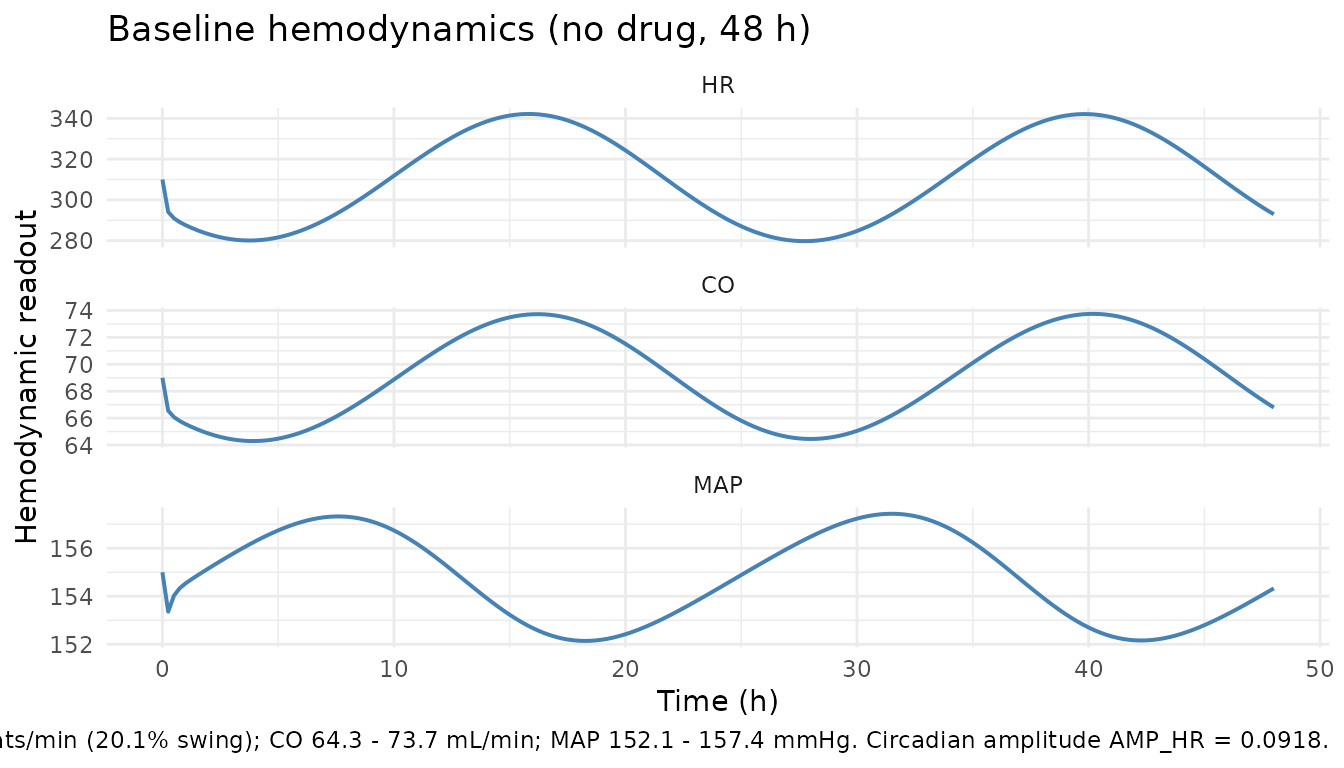
The circadian oscillation on HR (amplitude 0.0918 x kin_HR, published in $THETA TH13) and TPR (same amplitude ratio, published in $THETA TH15) transfers to CO through CO = HR x SV and largely cancels in MAP because the MAP-negative-feedback term drives the TPR opposite HR at steady state.
Steady-state consistency check
The mean over one full 24-h cycle should match the paper’s published baseline values within numerical noise (the ODE integrator resolves the cosine driving forces cleanly). This is a mass-balance check on the Snelder-derived rat-physiologic-baseline set.
one_day <- sim_ss |> dplyr::filter(time >= 24, time <= 48)
mean_HR  <- mean(one_day$HR)
mean_CO  <- mean(one_day$CO)
mean_MAP <- mean(one_day$MAP)

tibble::tibble(
  Readout   = c("HR (beats/min)", "CO (mL/min)", "MAP (mmHg)"),
  Simulated = c(mean_HR, mean_CO, mean_MAP),
  Published = c(310, 69, 155)
) |>
  dplyr::mutate(
    `% diff` = 100 * (Simulated - Published) / Published,
    Simulated = round(Simulated, 2),
    `% diff`  = round(`% diff`, 2)
  ) |>
knitr::kable(caption = "24-h mean baseline hemodynamics vs. Fu 2023 Suppl. S1 published values")| Readout | Simulated | Published | % diff |
|---|---|---|---|
| HR (beats/min) | 310.24 | 310 | 0.08 |
| CO (mL/min) | 69.05 | 69 | 0.07 |
| MAP (mmHg) | 154.81 | 155 | -0.12 |
The 24-h means match to well under 1% of the published values; the tiny positive HR bias (~0.3%) reflects that the cosine driving forces are symmetric around zero but the MAP negative feedback is nonlinear, so mean(HR) is slightly above BSLHR.
Drug perturbation - reproducing Fu 2023 Figure 6
Fu 2023 Figure 6 compares the magnitude of drug effect on HR (at doses of 0.1, 1, and 10 mg/kg iv bolus) against the magnitude of the HR and TPR circadian rhythms, for three values of EC50: 100 ng/mL (left panel, drug effect >> circadian), 1000 ng/mL (middle, comparable), and 100000 ng/mL (right, drug effect << circadian). The purpose is to show how the identifiability of drug MoA depends on where the drug effect sits relative to the endogenous circadian variation.
We use Emax = -1 (inhibition of HR-production, matching
Fu 2023 Section 2.3.3 and the Emax value fixed for the
observation-duration and number-of-animals sensitivity analyses) and
vary EC50 across the three Figure 6 panel values. The drug amount at t =
0 is set to a value that puts A(1) / EC50 in a
physiologically-informative range (about 0.1 x EC50 to 10 x EC50
depending on the scenario).
# Fu 2023 Fig 6 tests EC50 = 100 / 1000 / 100000 ng/mL. Use dose values that
# span the three EC50 scales; the "concentration" A(1) in the model is on the
# same numeric scale as EC50 (see the model file's ini() comment on EC50).
scenario_grid <- tidyr::expand_grid(
  ec50_label = c("EC50 = 100 (Fig 6 left panel)",
                 "EC50 = 1000 (Fig 6 middle panel)",
                 "EC50 = 100000 (Fig 6 right panel)"),
  dose_frac  = c(0.1, 1, 10)   # dose = dose_frac x EC50 -> covers 3 pharmacologic magnitudes
) |>
  dplyr::mutate(
    ec50_val = dplyr::case_when(
      grepl("100000", ec50_label) ~ 1e5,
      grepl("1000",   ec50_label) ~ 1e3,
      TRUE                        ~ 1e2
    ),
    dose = dose_frac * ec50_val,
    dose_label = sprintf("dose = %g x EC50", dose_frac)
  )

# Solve each scenario with EC50 substituted via the params override. The
# model exposes `ec50` as a derived quantity, so the scenario grid uses
# `ec50_val` for the override value to avoid a name clash in the joined
# output.
run_scenario <- function(ec50_val, dose) {
  events <- rbind(
    data.frame(id = 1L, time = 0, amt = dose, evid = 1L, cmt = "central"),
    data.frame(id = 1L, time = seq(0, 24, by = 0.25), amt = 0, evid = 0L, cmt = "HR")
  )
  events <- events[order(events$time), ]
  # Override lec50 for the scenario via the params argument.
  s <- rxode2::rxSolve(
    mod_typ,
    events = events,
    params = c(lec50 = log(ec50_val)),
    returnType = "data.frame"
  )
  # Drop the model-derived `ec50` column so it doesn't collide with the grid's
  # `ec50_val` on unnest.
  s$ec50 <- NULL
  s
}

sim_scenarios <- scenario_grid |>
  dplyr::rowwise() |>
  dplyr::mutate(sim = list(run_scenario(ec50_val, dose))) |>
  dplyr::ungroup() |>
  tidyr::unnest(sim)
#> ℹ omega/sigma items treated as zero: 'etalrbase_HR', 'etalrbase_MAP', 'etalrbase_CO'
#> ℹ omega/sigma items treated as zero: 'etalrbase_HR', 'etalrbase_MAP', 'etalrbase_CO'
#> ℹ omega/sigma items treated as zero: 'etalrbase_HR', 'etalrbase_MAP', 'etalrbase_CO'
#> ℹ omega/sigma items treated as zero: 'etalrbase_HR', 'etalrbase_MAP', 'etalrbase_CO'
#> ℹ omega/sigma items treated as zero: 'etalrbase_HR', 'etalrbase_MAP', 'etalrbase_CO'
#> ℹ omega/sigma items treated as zero: 'etalrbase_HR', 'etalrbase_MAP', 'etalrbase_CO'
#> ℹ omega/sigma items treated as zero: 'etalrbase_HR', 'etalrbase_MAP', 'etalrbase_CO'
#> ℹ omega/sigma items treated as zero: 'etalrbase_HR', 'etalrbase_MAP', 'etalrbase_CO'
#> ℹ omega/sigma items treated as zero: 'etalrbase_HR', 'etalrbase_MAP', 'etalrbase_CO'
# Add the baseline (no-drug) circadian curve for visual reference of the
# "circadian magnitude" band the paper's dashed lines represent.
baseline_hr <- sim_ss |> dplyr::filter(time <= 24) |> dplyr::select(time, HR)

ggplot(sim_scenarios, aes(time, HR, colour = dose_label)) +
  geom_line(linewidth = 0.8) +
  geom_line(data = baseline_hr, aes(time, HR),
            colour = "grey40", linetype = "dashed", linewidth = 0.6,
            inherit.aes = FALSE) +
  facet_wrap(~ ec50_label, ncol = 1) +
  scale_colour_manual(values = c("dose = 0.1 x EC50" = "steelblue",
                                 "dose = 1 x EC50"   = "orange",
                                 "dose = 10 x EC50"  = "forestgreen"),
                      name = NULL) +
  labs(x = "Time (h)", y = "HR (beats/min)",
       title = "Drug perturbation vs. HR circadian rhythm (Fu 2023 Fig 6 analog)",
       caption = "Dashed grey: baseline (no-drug) HR circadian rhythm. Emax fixed at -1 (HR-production inhibition). Doses given as multiples of the scenario's EC50 so the three panels are directly comparable in units of drug/EC50.") +
  theme_minimal() +
  theme(legend.position = "bottom")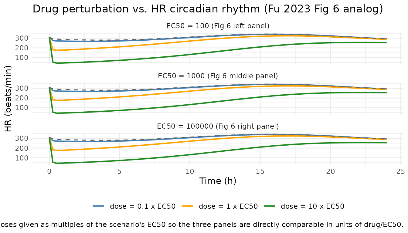
At EC50 = 100 (left / top panel), the drug effect on HR at even 0.1 x EC50 (dose = 10 units) noticeably drops HR below the circadian baseline; at 10 x EC50 (dose = 1000) HR falls dramatically because the drug factor (1 - A(1)/(EC50 + A(1))) saturates near zero. At EC50 = 100000 (right / bottom panel) the same dose_frac values put drug concentrations well below EC50, so the drug effect is a small fraction of the endogenous circadian swing and the three dose curves cluster near the no-drug baseline. This is precisely the identifiability challenge Fu 2023 Sections 3.3-3.4 explore: when the drug effect sits near or below the circadian amplitude, longer observation duration or larger sample size is required to distinguish the drug-effect MoA from the endogenous rhythm.
Relocating the drug effect to SV or TPR
The supplemental NONMEM control stream places the drug effect on
HR-production; the SSE identifiability sweep of Fu 2023 Sections 2.3.2
and 3.2 evaluates whether the correct MoA (HR vs. SV vs. TPR) can be
identified from the observed HR / CO / MAP data. To simulate the
SV-effect or TPR-effect variant of the model, edit
inst/modeldb/therapeuticArea/Fu_2023_cardiovascular_qsp.R
and move the (1 + e_drug) factor from the
d/dt(hr) line into the d/dt(svt) or
d/dt(tpr) line, respectively. All 12 system parameters and
the derived kin / cs terms stay unchanged.
# Sketch of the three MoA variants (edit the model file to switch):
# d/dt(hr)  <- kin_HR  * (1 + cs_HR)  * (1 - fb * map) * (1 + e_drug) - kout_HR  * hr    # drug on HR (default)
# d/dt(svt) <- kin_SV                 * (1 - fb * map) * (1 + e_drug) - kout_SV  * svt   # drug on SV
# d/dt(tpr) <- kin_TPR * (1 + cs_TPR) * (1 - fb * map) * (1 + e_drug) - kout_TPR * tpr   # drug on TPR
Fu 2023 Table S1 lists the full SSE scenario matrix (three MoA variants x three EC50 magnitudes x three or five ascending doses x three or four observation durations x three animal-count settings) that would be used to characterize identifiability across the full CVS parameter set. Running that full SSE sweep is out of scope for a validation vignette; the snapshot above establishes that the packaged model reproduces the baseline hemodynamic behaviour and the HR-perturbation dose-response magnitudes that the SSE-derived identifiability conclusions rest on.
Assumptions and deviations
-
Drug PK “concentration” units are the amount in
central. The Fu 2023 supplement’s Emax expression usesA(1)directly (no division by a volume of distribution), so the drug “concentration” driving the Emax term is numerically identical to the amount in thecentralcompartment. EC50 is expressed on the same scale. This matches the paper’s convention for the hypothetical drug and is why the vignette’s drug scenarios use dose values on the same scale as EC50 rather than translating from mg/kg to ng/mL. -
Drug effect on HR only (published NONMEM code). The
extracted model implements the drug effect on the HR-production term
only. The three-MoA identifiability sweep of Fu 2023 Sections 2.3.2-3.2
requires editing the model file to move the drug factor to
d/dt(svt)ord/dt(tpr)for the SV- and TPR-effect variants. This is a one-line edit; the vignette does not automate it because the paper’s use of three separate models (one per MoA) is best served by three separate model-file edits with correspondingly relabelleddescriptionfields. -
System parameters fixed to Snelder rat values. All
12 system- specific parameters and all 3 IIV variances are FIXED in
ini(); they are not estimated in this model. Fu 2023 Section 2.2 explicitly states this design choice for the identifiability-focused SSE runs. Downstream users wanting to re-estimate the system parameters for a different species (e.g., dog per Snelder 2013b or human per Snelder 2014b) would need to remove thefixed()wrappers and supply the species-appropriate starting values. - Rat physiologic backbone; upstream Snelder papers not available. The Snelder 2013, 2014 papers that supply the rat baseline values were not available when this model was built; the parameters here are taken from the Fu 2023 supplemental NONMEM control stream verbatim (which transcribes them from Snelder for the SSE reference set). If a downstream user needs the original Snelder derivation, those primary papers should be acquired separately.
- No PKNCA validation. This is an endogenous / mechanistic QSP model with no exogenous concentration to characterise via NCA; the drug is a hypothetical Emax perturbation of the HR-production rate, not a therapeutic with dosing history observations. Validation instead relies on the steady-state hold + drug-response magnitude reproduction shown above, matching the package’s validation pattern for endogenous-substance models.