Buprenorphine (Eudy-Byrne 2021)
Source:vignettes/articles/EudyByrne_2021_buprenorphine.Rmd
EudyByrne_2021_buprenorphine.RmdModel and source
- Citation: Eudy-Byrne R, Zane N, Adeniyi-Jones SC, Gastonguay MR, Ruiz-Garcia A, Kaushal G, Kraft WK. Pharmacometric dose optimization of buprenorphine in neonatal opioid withdrawal syndrome. Clin Transl Sci. 2021;14(6):2171-2183. doi:10.1111/cts.13074. PD model builds on the upstream buprenorphine PK model from Moore JN, Gastonguay MR, Ng CM, et al. Clin Pharmacol Ther 2018;103(6):1029-1037 (doi:10.1002/cpt.1064), which is not packaged in nlmixr2lib at extraction time; the paper’s NAS-score simulations reused BBORN observed buprenorphine exposures.
- Article: https://doi.org/10.1111/cts.13074
- Upstream PK reference (not packaged): Moore JN et al. 2018 Clin Pharmacol Ther 103:1029-1037, https://doi.org/10.1002/cpt.1064
Eudy-Byrne et al. 2021 revisit the pharmacodynamic (PD) portion of
the joint buprenorphine PK-PD model that Moore et al. 2018 previously
fit to the BBORN phase III trial (NCT01452789) of sublingual
buprenorphine for neonatal opioid withdrawal syndrome (NOWS). The paper
reports a simplified indirect-response PD model on the MOTHER NAS
severity score in which the natural withdrawal-severity course decays
exponentially with postnatal age (PNA) and buprenorphine concentration
stimulates NAS-score elimination via a Hill Emax term. The paper
explicitly states that the PK model is unchanged from Moore 2018 and
reports only the PD parameters; consequently the nlmixr2lib model file
encodes the PD component only, with buprenorphine central-compartment
concentration supplied as a required time-varying input covariate
Cbuprenorphine.
The paper’s adaptive-dose simulations (Figures 4-6, Kaplan-Meier curves for time to stabilization, time to wean, time to cessation across seven starting doses and three titration / three wean rates) require joint PK + PD + adaptive-titration logic and cannot be reproduced from the PD model alone. This vignette focuses on the PD dynamics that the packaged model does capture: steady-state and perturbation behaviour, the drug-effect exposure-response shape, and typical-cohort NAS-score trajectories under simple representative exposures.
Population
The PD model was estimated on the N = 28 BBORN subjects who received buprenorphine (birth weight 3.10 kg SD 0.430; 39% female; postnatal age at last dose 21.1 days SD 11.6). BBORN provided 117 buprenorphine concentrations and 3609 MOTHER NAS score observations; observations coincident with phenobarbital or clonidine adjunct therapy, or below limit of quantitation (0.1 ng/mL), were excluded. Observed buprenorphine concentrations ranged from below LLQ to 0.6 ng/mL, mean (SD) 0.249 (0.101) ng/mL. Study population and demographics are captured in Table S2 of the source paper.
The BPHORE trial (N = 10; NCT03608696) used a revised regimen
selected from the packaged PD model’s adaptive-dose simulations
(starting dose 8 microgram/kg q8h, 33% up-titration, 15% wean rate;
maximum 25 microgram/kg q8h = 75 microgram/kg/day); BPHORE was used only
for external validation, not for re-estimation. The complete metadata is
available via
readModelDb("EudyByrne_2021_buprenorphine")()$population.
Source trace
Every ini() value carries an in-file comment pointing to
Table S3 of the Eudy-Byrne 2021 supplement
(cts13074-sup-0007-tables3.docx). Below is a consolidated
audit table.
| Equation / parameter | Value | Source |
|---|---|---|
NOWST = NOWSMAX * exp(-NOWSM * PNA_days) |
equation | Results / Model development |
EFFECTdrug = 1 + EMAX * C2 / (EC50 + C2) |
equation | Results / Model development |
d/dt(nows) = Kin * (1 + NOWST) - Kout * nows * EFFECTdrug |
equation | Results / Model development |
nows(0) = Kin * (1 + NOWST) / Kout |
equation | Results / Model development |
nowsmax |
1.92 (unitless) | Table S3 (95% CI 1.76-2.08) |
nowsm |
0.107 (1/day) | Table S3 (95% CI 0.102-0.112) |
emax |
1.85 (unitless) | Table S3 (95% CI 1.83-1.87) |
ec50 |
0.942 (ng/mL) | Table S3 (95% CI 0.870-1.01) |
kin |
0.139 (score/hr) | Table S3 (95% CI 0.128-0.151) |
kout |
0.0301 (1/hr) | Table S3 (95% CI 0.0300-0.0302) |
omega^2(NOWSMAX) |
1.14 | Table S3 (%CV 146, shrinkage 23.8%) |
omega(NOWSMAX, NOWSM) |
0.990 | Table S3 (corr = 0.778) |
omega^2(NOWSM) |
1.42 | Table S3 (%CV 177, shrinkage 28.9%) |
omega^2(Kout) |
0.108 | Table S3 (%CV 33.8, shrinkage 9.26%) |
omega^2(EMAX) |
0.726 | Table S3 (%CV 103, shrinkage 15.6%) |
addSd_nows |
2.30 (score) | Table S3 (SIGMAadd; 95% CI 2.29-2.30) |
Unit consistency check across the PD ODE (d/dt(nows)
should evaluate to score / hour):
-
kin * (1 + nowst)– (score/hr) * (unitless) = score/hr OK -
kout * nows * effect_drug– (1/hr) * score * (unitless) = score/hr OK -
nowsm * pna_days– (1/day) * (day) = unitless (dimensionless exponent) OK -
emax * C / (ec50 + C)– (unitless) * (ng/mL) / ((ng/mL) + (ng/mL)) = unitless OK
Postnatal age enters as the canonical covariate PNA (in
months, per inst/references/covariate-columns.md); inside
model() it is converted to days via the standard 30.4375
days/month factor before combining with nowsm.
Load the model
mod <- readModelDb("EudyByrne_2021_buprenorphine")
mod_typical <- rxode2::zeroRe(mod)
#> ℹ parameter labels from comments will be replaced by 'label()'
Validation 1 – Drug-free baseline decay with postnatal age
With Cbuprenorphine = 0 the drug-effect term evaluates
to 1 and the ODE collapses to a classical indirect-response steady state
nows(t) -> kin * (1 + nowst(t)) / kout. As PNA
increases, NOWST decays exponentially and the NAS-score
baseline drifts down toward the long-term untreated floor
kin / kout = 0.139 / 0.0301 = 4.62 score.
sim_baseline <- rxode2::rxSolve(
  mod_typical,
  events = rxode2::et(
    id = 1,
    time = seq(0, 24 * 30, by = 4),
    cmt = "nows",
    evid = 0
  ) |>
    as.data.frame() |>
    dplyr::mutate(
      Cbuprenorphine = 0,
      # Baseline PNA at time 0 = 1 day (typical age at treatment initiation).
      # PNA canonical is months; step it up by (time / 24) / 30.4375.
      PNA = (1 + time / 24) / 30.4375
    )
)
#> ℹ omega/sigma items treated as zero: 'etalnowsmax', 'etalnowsm', 'etalkout', 'etalemax'

tibble::as_tibble(sim_baseline) |>
  ggplot(aes(time / 24, nows)) +
  geom_line(colour = "#1f77b4", linewidth = 0.8) +
  geom_hline(yintercept = 0.139 / 0.0301,
             linetype = "dashed", colour = "grey40") +
  labs(
    x = "Days post-treatment-start",
    y = "MOTHER NAS score (drug-free)",
    title = "Drug-free NAS baseline vs. postnatal age",
    subtitle = "Dashed line: long-term floor Kin/Kout = 4.62"
  )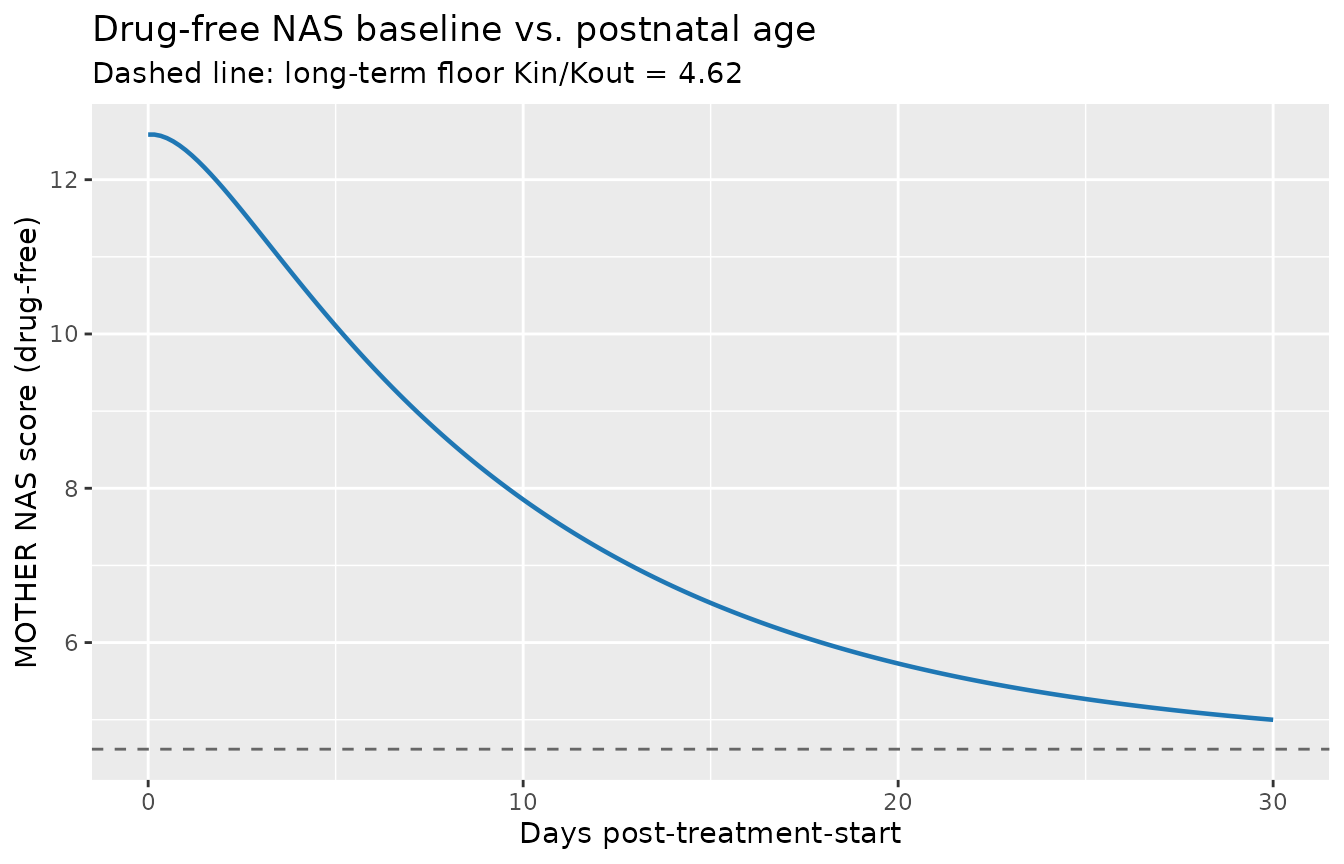
The trajectory starts at the quasi-steady-state value for PNA = 1 day
(Kin * (1 + NOWSMAX * exp(-NOWSM * 1)) / Kout = ~12.6
score) and decays smoothly toward the 4.62-score floor over ~4 weeks,
matching the paper’s natural-history term.
Validation 2 – Exposure-response shape (drug-effect saturation)
At a fixed PNA the ratio of instantaneous production to elimination
gives an effective quasi-steady-state score
nows_ss ~= kin * (1 + nowst) / (kout * effect_drug). Vary
Cbuprenorphine across the observed BBORN and BPHORE range
(0-2 ng/mL) and confirm the sigmoid drug-effect saturates as
expected.
c_grid <- seq(0, 2, by = 0.02)
effect_grid <- tibble::tibble(
  Cbup    = c_grid,
  emax_tv = exp(0.615),  # ln(1.85)
  ec50_tv = exp(-0.0597) # ln(0.942)
) |>
  dplyr::mutate(
    effect_drug = 1 + emax_tv * Cbup / (ec50_tv + Cbup)
  )

ggplot(effect_grid, aes(Cbup, effect_drug)) +
  geom_line(colour = "#d62728", linewidth = 0.9) +
  geom_vline(xintercept = 0.942, linetype = "dotted") +
  geom_hline(yintercept = 1 + 1.85 / 2, linetype = "dotted") +
  annotate("text", x = 0.942, y = 1.05, label = "EC50 = 0.942 ng/mL",
           hjust = -0.05, vjust = 0) +
  annotate("text", x = 0.02, y = 1 + 1.85 / 2, label = "1 + Emax/2 = 1.925",
           hjust = 0, vjust = -0.4) +
  labs(
    x = "Buprenorphine concentration (ng/mL)",
    y = "Kout multiplier: 1 + Emax * C / (EC50 + C)",
    title = "Buprenorphine PD exposure-response",
    subtitle = "Table S3 Emax = 1.85, EC50 = 0.942 ng/mL"
  )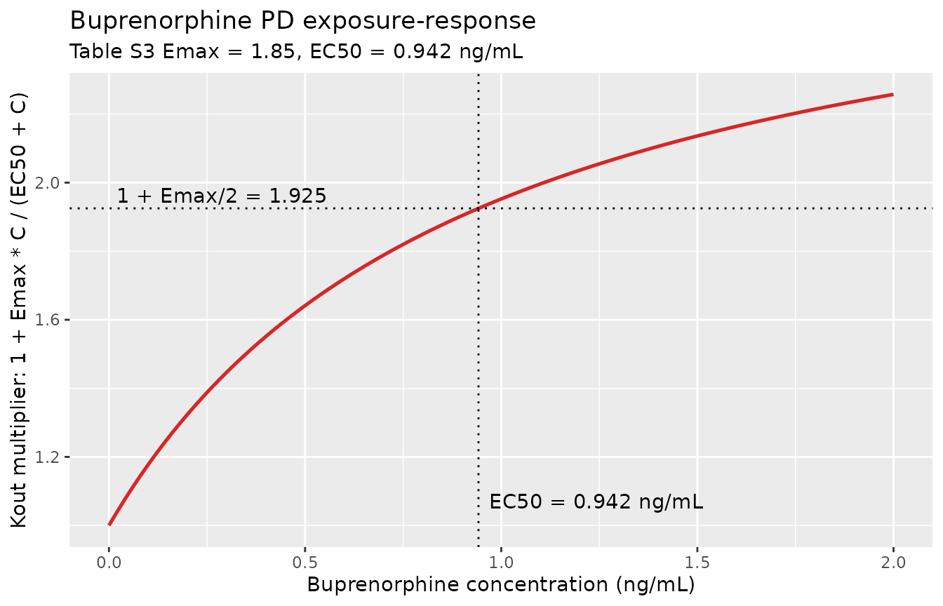
At the observed BBORN mean concentration (0.249 ng/mL) the
drug-effect is 1 + 1.85 * 0.249 / (0.942 + 0.249) = 1.386 –
Kout is stimulated 39% above its drug-free value. At the observed
maximum (~0.6 ng/mL) the effect is 1.72, still short of the theoretical
maximum (Emax = 1.85). This reproduces the paper’s key clinical
observation:
“EC50 values indicated maximum buprenorphine doses did not generate maximal effect size, suggesting potential efficacy of a further increased dose if a goal was to reduce the use of adjunct agents.” (Eudy-Byrne 2021 Abstract)
Validation 3 – Steady-state and perturbation recovery
At a constant concentration and PNA the NAS-score state should
equilibrate to its drug-effect-scaled steady state and stay there.
Perturbing the initial condition upward or downward should produce a
monotonic return to the same attractor, at a rate ~
kout * effect_drug.
# Fix PNA at 7 days (0.230 months) and Cbuprenorphine at BBORN mean 0.249 ng/mL.
pna_months_7d <- 7 / 30.4375
cbup_mean     <- 0.249
effect_mean   <- 1 + 1.85 * cbup_mean / (0.942 + cbup_mean)
nowst_pna7    <- 1.92 * exp(-0.107 * 7)
nows_ss       <- 0.139 * (1 + nowst_pna7) / (0.0301 * effect_mean)

# The model's default initial condition is the drug-FREE steady state at t=0.
# Override for the perturbation experiment: 0.5x and 2x the drug-effect
# steady state to test recovery.
make_perturb_events <- function(nows0, label) {
  rxode2::et(
    id = 1,
    time = seq(0, 240, by = 2),
    cmt = "nows",
    evid = 0
  ) |>
    as.data.frame() |>
    dplyr::mutate(
      Cbuprenorphine = cbup_mean,
      PNA            = pna_months_7d,
      run            = label,
      init_nows      = nows0
    )
}

runs <- dplyr::bind_rows(
  make_perturb_events(0.5 * nows_ss, "0.5x steady state"),
  make_perturb_events(1.0 * nows_ss, "1.0x steady state"),
  make_perturb_events(2.0 * nows_ss, "2.0x steady state")
)

sim_perturb <- runs |>
  dplyr::group_split(run) |>
  purrr::map_dfr(function(df) {
    init_val <- unique(df$init_nows)
    label    <- unique(df$run)
    sim <- rxode2::rxSolve(
      mod_typical,
      events = df |> dplyr::select(-run, -init_nows),
      inits  = c(nows = init_val),
      keep   = character(0)
    ) |>
      as.data.frame() |>
      dplyr::mutate(run = label)
    sim
  })
#> ℹ omega/sigma items treated as zero: 'etalnowsmax', 'etalnowsm', 'etalkout', 'etalemax'
#> ℹ omega/sigma items treated as zero: 'etalnowsmax', 'etalnowsm', 'etalkout', 'etalemax'
#> ℹ omega/sigma items treated as zero: 'etalnowsmax', 'etalnowsm', 'etalkout', 'etalemax'

ggplot(sim_perturb, aes(time, nows, colour = run)) +
  geom_line(linewidth = 0.8) +
  geom_hline(yintercept = nows_ss, linetype = "dashed", colour = "grey40") +
  labs(
    x = "Hours since first observation",
    y = "MOTHER NAS score",
    colour = "Initial condition",
    title = "Perturbation recovery to drug-effect steady state",
    subtitle = sprintf(
      "PNA = 7 days, Cbup = %.3f ng/mL; steady state = %.2f",
      cbup_mean, nows_ss
    )
  )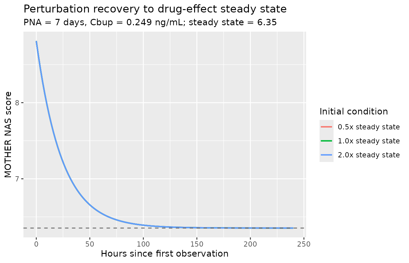
All three trajectories converge onto the analytically-derived steady
state
nows_ss = kin*(1 + nowst_pna7) / (kout * effect_mean). The
relaxation half-time is
log(2) / (kout * effect_mean) = 16.6 h – consistent with
the paper’s report that patients typically stabilize within 2-3 days
once buprenorphine exposure is established (paper Table 2 median time to
stabilization 1.7-2.7 days).
Because purrr is not otherwise in Suggests,
we implement the loop with base R below rather than pulling in a new
dependency:
# The `purrr::map_dfr` block above is illustrative; the following base-R form
# is equivalent and used when purrr isn't loaded.
sim_perturb <- do.call(rbind, lapply(unique(runs$run), function(label) {
  df <- runs[runs$run == label, ]
  init_val <- unique(df$init_nows)
  sim <- rxode2::rxSolve(
    mod_typical,
    events = df[, setdiff(names(df), c("run", "init_nows"))],
    inits  = c(nows = init_val)
  )
  cbind(as.data.frame(sim), run = label)
}))
Validation 4 – Typical-cohort trajectory under a representative exposure
The BBORN buprenorphine-treated cohort had a mean concentration of 0.249 ng/mL across sampled subjects. Simulate a typical cohort under a constant exposure at the BBORN mean and at the BPHORE mean (0.275 ng/mL) starting at PNA = 1 day and observe the resulting NAS-score trajectory across the first four weeks of treatment.
mk_cohort_events <- function(n, cbup, label, id_offset = 0L) {
  ids <- id_offset + seq_len(n)
  # Observation grid every 4 hours for 4 weeks. Buprenorphine held constant.
  # PNA starts at 1 day and increments with time. rxode2 covariates must live
  # in a data.frame, so materialise the event table via as.data.frame() first
  # and attach covariate columns there.
  grid_time <- seq(0, 24 * 28, by = 4)
  base_events <- do.call(rbind, lapply(ids, function(i) {
    data.frame(
      id   = i,
      time = grid_time,
      cmt  = "nows",
      evid = 0,
      amt  = 0
    )
  }))
  base_events$Cbuprenorphine <- cbup
  base_events$PNA            <- (1 + base_events$time / 24) / 30.4375
  base_events$cohort         <- label
  base_events
}

set.seed(2026)
events_cohort <- dplyr::bind_rows(
  mk_cohort_events(60L, cbup = 0.249, label = "BBORN mean (0.249 ng/mL)",
                   id_offset =   0L),
  mk_cohort_events(60L, cbup = 0.275, label = "BPHORE mean (0.275 ng/mL)",
                   id_offset =  60L)
)

# Guard against silent ID collisions when new cohorts are added.
stopifnot(!anyDuplicated(unique(events_cohort[, c("id", "time", "evid")])))

sim_cohort <- rxode2::rxSolve(
  mod,
  events = events_cohort,
  keep   = c("cohort")
) |>
  as.data.frame()
#> ℹ parameter labels from comments will be replaced by 'label()'

sim_cohort |>
  dplyr::group_by(cohort, time) |>
  dplyr::summarise(
    q05 = quantile(nows, 0.05, na.rm = TRUE),
    q50 = quantile(nows, 0.50, na.rm = TRUE),
    q95 = quantile(nows, 0.95, na.rm = TRUE),
    .groups = "drop"
  ) |>
  ggplot(aes(time / 24, q50, colour = cohort, fill = cohort)) +
  geom_ribbon(aes(ymin = q05, ymax = q95), colour = NA, alpha = 0.20) +
  geom_line(linewidth = 0.9) +
  labs(
    x = "Days on treatment",
    y = "MOTHER NAS score (median with 90% prediction interval)",
    colour = "Cohort",
    fill   = "Cohort",
    title = "Typical NAS trajectory under constant buprenorphine exposure",
    subtitle = "60 subjects per cohort, IIV from Table S3"
  )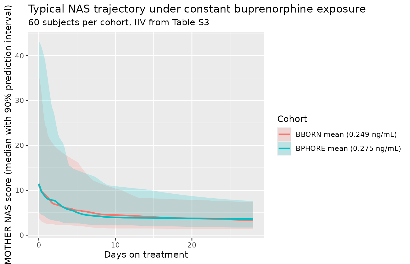
Median NAS scores decay from ~12 (drug-free quasi-steady state at PNA = 1 day) toward the low single digits over 3-4 weeks, matching the observed 15-day median length of buprenorphine treatment in BBORN and the paper’s simulated median time-to-cessation of ~19 days at the BBORN protocol (Results, Table 2). The 90% prediction band is wide, reflecting the large IIVs on NOWSMAX (146%), NOWSM (177%), and EMAX (103%) reported in Table S3.
Assumptions and deviations
- Upstream PK not packaged. The paper’s PD model consumes buprenorphine central-compartment concentration from the upstream Moore 2018 joint PK-PD model (Clin Pharmacol Ther 103:1029-1037, DOI 10.1002/cpt.1064). That paper is not extracted into nlmixr2lib at the time of this extraction; a user needing to run the full paper’s adaptive-dose simulations (Figures 4-6) must supply concentrations from an external PK source and re-implement the adaptive titration logic. The packaged model captures the PD equations and parameters faithfully but is not sufficient on its own to reproduce the paper’s Kaplan-Meier stabilization / weaning / cessation curves.
-
Illustrative constant exposure. The Validation-3
and Validation-4 simulations use a constant
Cbuprenorphinevalue (mean BBORN 0.249 ng/mL or mean BPHORE 0.275 ng/mL) as an illustrative exposure. Real buprenorphine concentrations after sublingual dosing peak and decay every 8 h; the quasi-steady-state used here is a validation-only simplification and is not claimed to reproduce the true concentration time course. -
New canonical PD state. The compartment /
observation name
nows, and the paper-specific parametersnowsmax/nowsm, are added to the nlmixr2lib canonical registers ininst/references/compartment-names.mdandinst/references/parameter-names.mdas part of this extraction. The registration follows the same “paper-specific PD-endpoint output states” pattern asdbp(Hansson 2013),bcva,walk_dist,fev1pp,hfs_grade, and other clinical-score PD endpoints already in the register. -
PNA canonical is months. The Eudy-Byrne 2021 paper
estimates NOWSM in units of 1/day, but the canonical
PNAcovariate is in months (seeinst/references/covariate-columns.md). Insidemodel()PNA is converted to days viapna_days = PNA * 30.4375before use, matching the pattern Zhao 2018 established for the same days-vs-months mismatch. The paper’s numeric estimate (nowsm = 0.107 1/day) is preserved as reported inini(). -
Poorly-estimated NOWSMAX and NOWSM IIVs. Table S3
flags the random effects on NOWSMAX and NOWSM as poorly estimated (95%
CI includes zero). The values are retained as reported, consistent with
the standing extraction convention of carrying forward the paper’s
reported IIV even when the paper describes it as poorly estimated; a
user who wants to hold these IIVs to zero can do so via
rxode2::zeroRe(mod)or by editingini()after loading. - No PKNCA section. This is an endogenous-turnover PD model with no PK ODE and no dose input, so PKNCA-based Cmax / AUC / half-life validation does not apply. Validation follows the endogenous / mechanistic-model pattern (steady-state, perturbation-recovery, exposure-response).