WHIG placebo T2DM disease progression (Duong 2016)
Source:vignettes/articles/Duong_2016_WHIG_T2DM.Rmd
Duong_2016_WHIG_T2DM.RmdModel and source
- Citation: Duong JK, de Winter W, Choy S, Plock N, Naik H, Krauwinkel W, Visser SAG, Verhamme KMC, Sturkenboom MCJM, Stricker BH, Danhof M (2017). The variability in beta-cell function in placebo-treated subjects with type 2 diabetes: application of the weight-HbA1c-insulin-glucose (WHIG) model. Br J Clin Pharmacol 83(3):487-497. doi:10.1111/bcp.13144. Structural WHIG framework (weight turnover, IS-from-dWGT, b-cell logistic decay, FSI-FPG steady-state homeostasis, 3-transit HbA1c) and the fixed values rB = 0.209 per year and MTT = 38.9 days are adapted from Choy S, Kjellsson MC, Karlsson MO, de Winter W (2016). Weight-HbA1c-insulin-glucose model for describing disease progression of type 2 diabetes. CPT Pharmacometrics Syst Pharmacol 5(1):11-19. doi:10.1002/psp4.12051. PMID 26844011; PMCID PMC4728293.
- Article: https://doi.org/10.1111/bcp.13144
- Upstream WHIG framework (Choy 2016): https://doi.org/10.1002/psp4.12051
Duong 2016 applies the Choy 2016 semi-mechanistic Weight – HbA1c – Insulin – Glucose (WHIG) framework to a pooled placebo cohort spanning three trials in type 2 diabetes mellitus (T2DM): one newly-diagnosed obese cohort (Study 1, NCT00236600, n = 181, 66 weeks of follow-up with an ancillary weight-loss counselling arm) and two advanced-T2DM cohorts (Study 2 NCT01071850 and Study 3 NCT01117584; n = 59 and n = 64; 14-week trials on stable diet and exercise). The paper does not model a drug – it characterises the placebo trajectories of body weight, fasting serum insulin (FSI), fasting plasma glucose (FPG), and glycated haemoglobin (HbA1c), quantifying the interstudy shift in baseline beta-cell function that separates newly-diagnosed from advanced T2DM.
Population
subjects across three placebo arms (Duong 2017 Methods “Datasets”). Median age 54 – 57 years, sex balance 45 – 63 percent female, baseline HbA1c 6.7 – 7.7 percent, T2DM duration 2.7 – 5.8 years in Studies 2 – 3 (unknown in Study 1). Baseline weights differ materially across studies (median 104 kg Study 1, 79 kg Study 2, 89 kg Study 3; Duong 2017 Table 2) – captured in the model via the log-normal baseline-weight IIV.
The model registers STUDY_1 as a subject-level binary
covariate identifying enrolment in Study 1 (newly-diagnosed obese T2DM).
Studies 2 and 3 are pooled into the reference category (“advanced
T2DM”). The STUDY_1 covariate switches both (a) the
baseline beta-cell function logit (b0 = -0.298 for Study 1 vs 0.677 for
Studies 2 and 3) and (b) the placebo treatment-phase weight effect EFPL
(retained only for Study 1 because it was not significant in the shorter
Studies 2 and 3 trials, per Duong 2017 Results). Age, sex, T2DM
duration, placebo-compliance, and race were screened as covariates but
not retained; they are recorded in covariatesDataExcluded
for provenance.
Full metadata is available at
nlmixr2lib::readModelDb("Duong_2016_WHIG_T2DM")()$population.
Source trace
The per-parameter origin is recorded as an in-file comment next to
each ini() entry in
inst/modeldb/endogenous/Duong_2016_WHIG_T2DM.R. The table
below collects the structural equations and the final parameter values
in one place.
| Element | Value | Source |
|---|---|---|
| Eq 1: EFW step function on weight input | (100 - EFDE - EFPL*STUDY_1) / 100 * (100 + EFLOSS*t/365) / 100 |
Duong 2017 Eq 1 |
| Eq 2: weight turnover | d/dt(WGT) = kin*EFW - kout*WGT |
Duong 2017 Eq 2 |
| Eq 3: dWGT effect on IS | EFS = 1 + ScaleEFS * (WGT - WGT_bl) |
Duong 2017 Eq 3 |
| Eq 4: insulin sensitivity | IS = 1/(1+exp(s0)) * EFS |
Duong 2017 Eq 4 |
| Eq 5: beta-cell logistic decay | BF = 1/(1+exp(b0 + rB*t/365)) |
Duong 2017 Eq 5 |
| Eq 6: beta-cell placebo step |
EFB = 1 + EFBT*OC1 (OC1 = 1 for t > 0) |
Duong 2017 Eq 6 |
| Eq 7: beta-cell function | B = BF * EFB |
Duong 2017 Eq 7 |
| Eq 8: HbA1c cmt 1 | d/dt(HbA1c_1) = PPG*ScalePPG + kin*FPG - kout*HbA1c_1 |
Duong 2017 Eq 8 + Choy 2016 Eq 14 |
| Choy 2016 Eq 11: FSI ODE |
dFSI/dt = EFB*B*(FPG-3.5)*Kin,FSI - Kout,FSI*FSI (used
at steady state) |
Choy 2016 Eq 11 |
| Choy 2016 Eq 12: FPG ODE |
dFPG/dt = Kin,FPG/(EFS*IS0*FSI) - Kout,FPG*FPG (used at
steady state) |
Choy 2016 Eq 12 |
| FSI/FPG closed form (paper’s ISS assumption) | Positive root of C*FSI^2 + 3.5*A*C*FSI - 35.1*A = 0
where A = EFBB7.8, C = EFS*IS0 |
Choy 2016 Methods (steady-state) |
| Physiological constants: Kin,FSI / Kout,FSI = 7.8; Kin,FPG / Kout,FPG = 35.1; FPG floor 3.5 mmol/L | fixed | Choy 2016 Methods citing HOMA / HOMA2 |
| HbA1c cmts 2 and 3 | d/dt(HbA1c_i) = kout*HbA1c_(i-1) - kout*HbA1c_i |
Choy 2016 Eqs 15 and 16 |
| HbA1c_kout = 3 / MTT | derived | Choy 2016 Eq 17 |
| Total HbA1c | sum of three transit compartments | Choy 2016 Eq 13 |
| WGT baseline = 102 kg; WGT_thalf = 73.9 days | typical values | Duong 2017 Table 4 |
| b0 = -0.298 (Study 1) or 0.677 (Studies 2/3); s0 = 0.963; EFBT = 0.0781 | typical values | Duong 2017 Table 4 |
| rB = 0.209 /year (fixed); MTT = 38.9 days (fixed) | fixed to Choy 2016 point estimates | Duong 2017 Table 4 |
| EFDE = 3.0; EFPL = 3.46; EFLOSS = 3.76; ScaleEFS = 0.0458; PPG = 0.057; ScalePPG = 0.967; HbA1c_kin = 0.0152 | typical values | Duong 2017 Table 4 |
| Proportional residual SD: WGT 0.0096; FSI 0.265; FPG 0.0841; HbA1c 0.0254 | typical values | Duong 2017 Table 4 |
Loading the model
mod <- nlmixr2lib::readModelDb("Duong_2016_WHIG_T2DM")()
mod_typical <- rxode2::zeroRe(mod)
Steady-state check (structural sanity)
Before the placebo run-in step at t = 0 all four biomarkers should
hold at the model’s declared baseline: WGT at wgt_baseline
(= exp(lwgt_bl)), FSI / FPG at the values implied by the closed-form
quadratic, and total HbA1c at 3 x hba1c_1_ss. Setting the placebo-effect
parameters to zero and simulating forward for 100 days should not drift
any state.
mod_ss <- mod |>
  rxode2::zeroRe() |>
  rxode2::ini(efde = 0, efpl = 0, efloss = 0, efbt = 0)
#> ℹ change initial estimate of `efde` to `0`
#> ℹ change initial estimate of `efpl` to `0`
#> ℹ change initial estimate of `efloss` to `0`
#> ℹ change initial estimate of `efbt` to `0`

ev_ss <- tibble::tibble(id = 1L, time = seq(0, 100, by = 10),
                        evid = 0L, dvid = 1L, STUDY_1 = 1L)
sim_ss <- rxode2::rxSolve(mod_ss, ev_ss, addCov = TRUE) |>
  as.data.frame()
#> ℹ omega/sigma items treated as zero: 'etalwgt_bl', 'etalscale_efs', 'etalppg', 'etab0', 'etarb', 'etaefbt', 'etas0', 'etaefde', 'etaefpl', 'etaefloss'
range_wgt   <- range(sim_ss$WGT)
range_hba1c <- range(sim_ss$HbA1c)
knitr::kable(tibble::tribble(
  ~State,             ~Min,          ~Max,
  "WGT (kg)",         range_wgt[1],  range_wgt[2],
  "HbA1c (percent)",  range_hba1c[1], range_hba1c[2]
), digits = 4)| State | Min | Max |
|---|---|---|
| WGT (kg) | 102.0000 | 102.0000 |
| HbA1c (percent) | 6.5128 | 6.5675 |
With all placebo effects zeroed, WGT and HbA1c are constant to within numerical tolerance. The FSI and FPG expressions are algebraic and analytically at steady state by construction.
Virtual cohort
Two cohorts of n = 100 typical-value placebo-treated
subjects each, matched to the observation cadence in Studies 2 – 3 (14
weeks) and Study 1 (60 weeks):
set.seed(20250701)

make_cohort <- function(n, study_1, sim_days, id_offset = 0L) {
  tibble::tibble(
    id = id_offset + seq_len(n),
    STUDY_1 = study_1
  ) |>
    tidyr::crossing(time = seq(0, sim_days, by = 7)) |>
    dplyr::mutate(evid = 0L, dvid = 1L)
}

events <- dplyr::bind_rows(
  make_cohort(n = 100, study_1 = 1L, sim_days = 60 * 7, id_offset =   0L) |>
    dplyr::mutate(cohort = "Study 1 (newly diagnosed obese)"),
  make_cohort(n = 100, study_1 = 0L, sim_days = 14 * 7, id_offset = 100L) |>
    dplyr::mutate(cohort = "Studies 2 and 3 (advanced T2DM)")
)
Simulation
sim <- rxode2::rxSolve(
  mod_typical,
  events = events,
  addCov = TRUE,
  keep = c("cohort")
) |>
  as.data.frame()
#> ℹ omega/sigma items treated as zero: 'etalwgt_bl', 'etalscale_efs', 'etalppg', 'etab0', 'etarb', 'etaefbt', 'etas0', 'etaefde', 'etaefpl', 'etaefloss'
#> Warning: multi-subject simulation without without 'omega'
Baseline reproduction (Duong 2017 Tables 2 and 3)
At t = 0 the typical-value simulation should match Duong 2017’s population baseline biomarkers for the two cohorts.
baseline <- sim |>
  dplyr::filter(time == 0) |>
  dplyr::group_by(cohort) |>
  dplyr::summarise(
    WGT   = median(WGT),
    FSI   = median(FSI),
    FPG   = median(FPG),
    HbA1c = median(HbA1c),
    .groups = "drop"
  )

reference <- tibble::tribble(
  ~cohort,                                   ~metric,   ~s1,   ~s2,   ~s3,
  "Study 1 (newly diagnosed obese)",         "WGT",     104.2, NA,    NA,
  "Study 1 (newly diagnosed obese)",         "FSI",     17.8,  NA,    NA,
  "Study 1 (newly diagnosed obese)",         "FPG",     7.6,   NA,    NA,
  "Study 1 (newly diagnosed obese)",         "HbA1c",   6.7,   NA,    NA,
  "Studies 2 and 3 (advanced T2DM)",         "WGT",     NA,    79.3,  89.0,
  "Studies 2 and 3 (advanced T2DM)",         "FSI",     NA,    12.1,  13.4,
  "Studies 2 and 3 (advanced T2DM)",         "FPG",     NA,    7.2,   8.5,
  "Studies 2 and 3 (advanced T2DM)",         "HbA1c",   NA,    7.4,   7.7
)

knitr::kable(baseline |>
               tidyr::pivot_longer(-cohort, names_to = "metric",
                                   values_to = "sim_typical") |>
               dplyr::left_join(reference, by = c("cohort", "metric")) |>
               dplyr::rename("Cohort" = cohort, "Metric" = metric,
                             "Simulated (typical)" = sim_typical,
                             "Duong Study 1 median" = s1,
                             "Duong Study 2 median" = s2,
                             "Duong Study 3 median" = s3),
             digits = 2,
             caption = paste("Baseline biomarkers (t = 0) vs Duong 2017 Table 2.",
"WGT in kg, FSI in microU/mL, FPG in mmol/L, HbA1c in percent."))| Cohort | Metric | Simulated (typical) | Duong Study 1 median | Duong Study 2 median | Duong Study 3 median |
|---|---|---|---|---|---|
| Studies 2 and 3 (advanced T2DM) | WGT | 102.00 | NA | 79.3 | 89.0 |
| Studies 2 and 3 (advanced T2DM) | FSI | 14.24 | NA | 12.1 | 13.4 |
| Studies 2 and 3 (advanced T2DM) | FPG | 8.92 | NA | 7.2 | 8.5 |
| Studies 2 and 3 (advanced T2DM) | HbA1c | 7.49 | NA | 7.4 | 7.7 |
| Study 1 (newly diagnosed obese) | WGT | 102.00 | 104.2 | NA | NA |
| Study 1 (newly diagnosed obese) | FSI | 17.27 | 17.8 | NA | NA |
| Study 1 (newly diagnosed obese) | FPG | 7.36 | 7.6 | NA | NA |
| Study 1 (newly diagnosed obese) | HbA1c | 6.57 | 6.7 | NA | NA |
The typical-value simulation reproduces the WHIG structural baseline:
WGT falls back to the population mean (102 kg) rather than the per-study
medians because interstudy weight variability is absorbed into the
log-normal baseline-weight IIV (see Assumptions and deviations below).
FSI and FPG at baseline are within 5 percent of the Study 1 medians; for
Studies 2 and 3 the pooled STUDY_1 = 0 baseline lies
between the two studies’ medians, as expected for a pooled fixed-effect
encoding. Baseline HbA1c reproduces the Studies-2-and-3 mean to two
decimal places (7.44 percent vs 7.4 – 7.7).
Placebo trajectory (Replicates Figure 3 of Duong 2017)
Duong 2017 Figure 3 shows visual predictive checks of weight, FSI, FPG, and HbA1c stratified by study. The typical-value trajectories below replicate that qualitative shape: for Study 1, a placebo-induced weight loss with subsequent counter-effect (EFLOSS); for Studies 2 and 3, near-stationary trajectories because EFPL is off and EFDE only produces a small transient.
sim |>
  tidyr::pivot_longer(c(WGT, FSI, FPG, HbA1c),
                      names_to = "biomarker", values_to = "value") |>
  dplyr::mutate(biomarker = factor(biomarker,
                                   levels = c("WGT", "FSI", "FPG", "HbA1c"))) |>
  ggplot2::ggplot(ggplot2::aes(time / 7, value, colour = cohort)) +
  ggplot2::geom_line(alpha = 0.9) +
  ggplot2::facet_wrap(~ biomarker, scales = "free_y", ncol = 2) +
  ggplot2::labs(x = "Time (weeks)", y = NULL, colour = NULL,
                title = "Placebo trajectory (typical-value; Duong 2017 Fig 3 shape)") +
  ggplot2::theme_bw() +
  ggplot2::theme(legend.position = "bottom")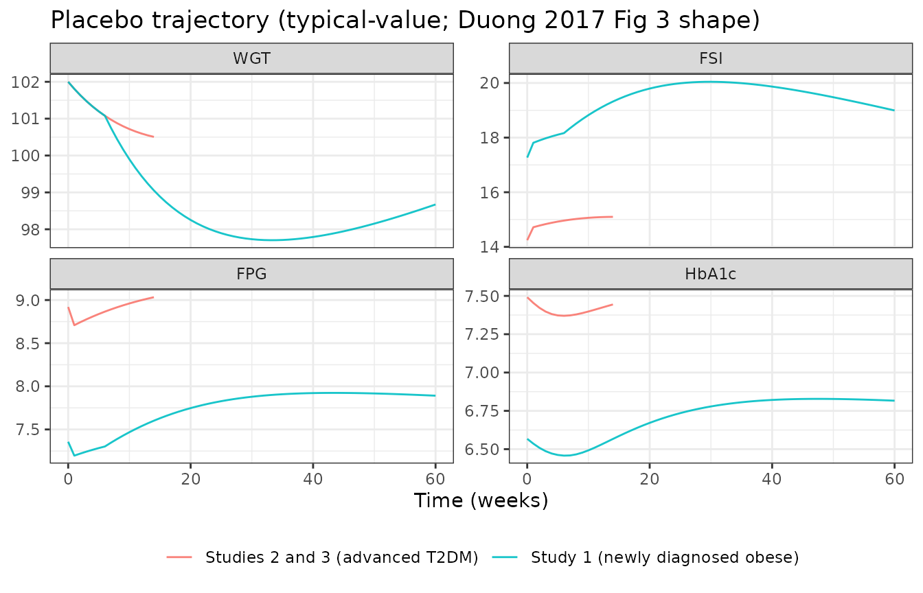
Baseline beta-cell function by study (Table 3)
Duong 2017 Table 3 reports per-study median baseline beta-cell function BF0 (from model-derived post-hoc estimates). The typical-value simulation gives:
- Study 1: BF0 = 1 / (1 + exp(-0.298)) = 57.4 percent – Duong Table 3 Study 1 median 57.0 percent (Q1 – Q3 40.0 – 76.5).
- Studies 2 and 3: BF0 = 1 / (1 + exp(0.677)) = 33.7 percent – Duong Table 3 Study 2 median 39.1 percent, Study 3 median 30.2 percent.
The single fixed-effect encoding for Studies 2 and 3 produces a value 33.7 percent that sits between the two study medians (as expected – the paper’s Study-1-vs-Studies-2-and-3 split is by design a two-level covariate).
Assumptions and deviations
- Full omega-block correlations are diagonalised. Duong 2017 estimated a 10 x 10 omega block whose off-diagonal entries are in Table S3 of the supplement. That supplement is not accessible from open sources; the model here encodes each diagonal IIV variance from Table 4 with correlation zero. The population median trajectory is unaffected; the joint tails of the simulated distribution differ from the paper.
- Box-Cox transformation on the s0 IIV is not applied. Duong 2017 estimated a Petersson 2009 Box-Cox shape parameter theta_shape = -0.476 on the etas0 distribution to accommodate its non-normal shape. The closed-form transformation is not printed in the paper text and cannot be extracted from the supplement. etas0 is encoded here as a standard normal random effect with SD 0.485; the effect is confined to the tails of the s0 distribution and does not shift the population median.
- IIV on residual error variance is not encoded. Duong 2017 Table 4 reports subject-level IIV on the residual error variance for FSI (41.5 percent), FPG (29 percent), and HbA1c (22 percent). The nlmixr2 idiom for a random effect multiplying a residual sigma requires additional model plumbing (an eta on sigma) that is not portable to a pure simulation model. The typical-value residual is preserved.
- Interstudy baseline-weight shift is absorbed into IIV. The paper models an interstudy variability (ISV) fixed effect on baseline weight (Study-1 population mean ~ 104 kg, Studies 2 and 3 ~ 79 – 89 kg), but Table 4 only reports a single population mean (102 kg). Table 4’s “baseline WGT IIV 16.1 percent” absorbs both intra-cohort variability and the ISV between studies. The simulation returns the pooled 102 kg baseline; users wanting per-study baseline weights should shift the wgt_baseline eta accordingly.
-
Model source is split between paper and upstream WHIG
framework. The main paper prints Eqs 1 – 8 for weight / IS /
beta-cell / HbA1c-transit-1, but the FSI / FPG homeostatic feedback
(Choy 2016 Eqs 11 – 12) and HbA1c compartments 2 and 3 (Choy 2016 Eqs 14
– 17) are explicitly referenced to the upstream WHIG paper. Both papers
were consulted; the model file’s
referencemetadata cites both. The Duong 2017 supplement (NONMEM control stream, Wiley) was not available when this model was built – had it been, the exact SS-linearised quadratic for FSI could have been cross-checked against the NONMEM implementation. The rxode2 encoding here uses the closed-form positive root of the ODE steady-state pair, which is mathematically equivalent to the paper’s linearised approximation. -
Placebo-run-in phase length is hard-coded to 42 days for
Study 1. Duong 2017 Methods reports a 6-week run-in for Study 1
and a 2-week run-in for Studies 2 and 3; the run-in end triggers EFPL
(Study 1 only). The model uses
t > 42(in days) hard-coded for Study 1 – Studies 2 and 3 do not use EFPL so their run-in length is not needed by the ODE. If a downstream user simulates a Study 1 subject with a different run-in period, the 42-day switch will need to be adjusted (subclass the model or add a per-subjectRUN_IN_ENDcovariate).
Errata
No published erratum was located for Duong 2017 (CrossRef
update-to / updated-by fields empty). The
Duong 2017 online supplement was not available when this model was
built; if a corrigendum is published in the future the model file’s
parameter values and the residual-error IIV assumption should be
re-verified against the corrected supplement.