Motesanib tumor size and overall survival in NSCLC (Claret 2014)
Source:vignettes/articles/Claret_2014_motesanib_nsclc.Rmd
Claret_2014_motesanib_nsclc.RmdModel and source
This paper contributes two models to the library.
tso <- rxode2::rxode(readModelDb("Claret_2014_motesanib_tumorsize_OS"))
#> ℹ Joint TS/OS exploratory model for first-line nonsquamous NSCLC (Claret 2014 MONET1, n=934 TS-evaluable). TS = simplified Claret TGI with resistance decay (kge, kdrug, lambda, rbase); OS = log-normal AFT driven by log(TTG+100) plus baseline TS, RACE_ASIAN and smoking history. Outputs: tumor_size (observable, mm), ttg, log_ttg, mu_os_logdays, sigma_os, median_os, sur, hazard, cumhazard. ERRATUM: Supplementary Table S1 transposes the KDE and lambda estimates; this model uses the corrected KDE=0.0103, lambda=0.0193 per day, which is what reproduces the paper's own published TTG and TSratio medians. The TS sub-model has NO treatment-arm term, so fresh-eta simulation gives the same TTG distribution in both arms; the paper conditioned its trial simulations on observed per-patient TTG instead. log(TTG+100) is undefined for TTG <= -100 days and is deliberately left unguarded. Companion model for TS-nonevaluable patients: modellib('Claret_2014_motesanib_OS_nonevaluable').
#> ℹ parameter labels from comments will be replaced by 'label()'
nev <- rxode2::rxode(readModelDb("Claret_2014_motesanib_OS_nonevaluable"))
#> ℹ Log-normal AFT overall-survival model for the tumor-size-NONEVALUABLE MONET1 patients (Claret 2014, n=146). Baseline serum albumin (ALB, g/L, uncentred) is the sole prognostic factor; there is no drug-effect term, no tumor-size term, no ODE, no IIV and no residual error. Outputs: mu_os_logdays, sigma_os, median_os, sur, hazard, cumhazard. Use it to correct trial simulations built on modellib('Claret_2014_motesanib_tumorsize_OS') for the 14 percent nonevaluable fraction, as the source paper did.- Citation: Claret L, Bruno R, Lu J-F, Sun Y-N, Hsu C-P. Exploratory modeling and simulation to support development of motesanib in Asian patients with non-small cell lung cancer based on MONET1 study results. Clin Pharmacol Ther. 2014;95(4):446-451. doi:10.1038/clpt.2014.11. TS model parameter estimates: Supplementary Table S1. OS model parameter estimates: Table 3; parameter covariance matrix: Supplementary Table S3. The companion model for TS-nonevaluable patients is modellib(‘Claret_2014_motesanib_OS_nonevaluable’).
- Article: https://doi.org/10.1038/clpt.2014.11
Claret_2014_motesanib_tumorsize_OS –
the joint tumor-size (TS) / overall-survival (OS) model for the 934
TS-evaluable patients.
Claret_2014_motesanib_OS_nonevaluable –
the separate OS model for the patients whose tumor-size response could
not be predicted, which the authors used to correct their trial
simulations for the nonevaluable fraction.
A third model is discussed in the paper but is not extractable from it: the “historical” first-line NSCLC OS model of Wang et al., which Claret 2014 assesses and then improves upon. Its parameter estimates live in that earlier publication and are not reprinted here, so no model file is created for it.
Population
MONET1 randomised 1,090 patients with advanced or recurrent nonsquamous NSCLC to carboplatin/paclitaxel (CP) plus motesanib 125 mg once daily or CP plus placebo, first line. Of these, 934 (86%) were TS-evaluable – 453 of 541 on motesanib and 481 of 549 on placebo – with a median of four TS measurements per patient (range 2-27). The remaining 156 (14%) were nonevaluable: 115 had no postbaseline tumor assessment and 41 had only nontarget lesions. 227 enrolled patients (21%) were Asian; the 219 Asian patients used for the virtual phase III simulations included 21 nonevaluable patients.
The same information is available programmatically from each model’s
population metadata:
str(readModelDb("Claret_2014_motesanib_tumorsize_OS")()$population[
  c("n_subjects", "disease_state", "race_ethnicity")
])
#> ℹ Joint TS/OS exploratory model for first-line nonsquamous NSCLC (Claret 2014 MONET1, n=934 TS-evaluable). TS = simplified Claret TGI with resistance decay (kge, kdrug, lambda, rbase); OS = log-normal AFT driven by log(TTG+100) plus baseline TS, RACE_ASIAN and smoking history. Outputs: tumor_size (observable, mm), ttg, log_ttg, mu_os_logdays, sigma_os, median_os, sur, hazard, cumhazard. ERRATUM: Supplementary Table S1 transposes the KDE and lambda estimates; this model uses the corrected KDE=0.0103, lambda=0.0193 per day, which is what reproduces the paper's own published TTG and TSratio medians. The TS sub-model has NO treatment-arm term, so fresh-eta simulation gives the same TTG distribution in both arms; the paper conditioned its trial simulations on observed per-patient TTG instead. log(TTG+100) is undefined for TTG <= -100 days and is deliberately left unguarded. Companion model for TS-nonevaluable patients: modellib('Claret_2014_motesanib_OS_nonevaluable').
#> List of 3
#>  $ n_subjects    : int 934
#>  $ disease_state : chr "Advanced (stage IIIB with pleural effusion or stage IV) or recurrent nonsquamous non-small cell lung cancer, pr"| __truncated__
#>  $ race_ethnicity: chr "227 of the 1,090 enrolled MONET1 patients (21 percent) were Asian; 219 Asian patients were resampled for the vi"| __truncated__
Source trace
Every ini() value carries an in-file comment naming its
source location. They are collected here for review.
| Equation / parameter | Value | Source location |
|---|---|---|
TS(t) = BASE * exp(KL*t - (KDE/lambda)*(1 - exp(-lambda*t))) |
n/a | Methods, “TS model” (p. 450, left column) |
d/dt(tumor_size) = tumor_size * (kge - kdrug*exp(-lambda*t)) |
n/a | Derivative of the Methods TS equation (see “Structural checks” below) |
TSratio = TS(week8) / BASE |
n/a | Methods, “Two metrics to assess TS response”, metric 1 |
TTG = (log(KDE) - log(KL)) / lambda |
n/a | Methods, metric 2 |
log(TTG*) = log(TTG + 100) |
n/a | Methods, shifted-log definition |
lrbase (BASE) |
90 mm | Supplementary Table S1 (RSE 2.37%) |
lkge (KL) |
0.00107 /day | Supplementary Table S1 (RSE 7.70%) |
lkdrug (KDE) |
0.0103 /day | Supplementary Table S1, estimate read off the lambda row (RSE 5.16% from the KDE row); see “Supplementary Table S1 transposes KDE and lambda” and Errata item 1 |
llambda (lambda) |
0.0193 /day | Supplementary Table S1, estimate read off the KDE row (RSE 3.72% from the lambda row); see “Supplementary Table S1 transposes KDE and lambda” and Errata item 1 |
etalrbase |
SD 0.683 -> var 0.4665 | Supplementary Table S1, “SD” column |
etalkge |
SD 1.18 -> var 1.3924 | Supplementary Table S1, “SD” column |
etalkdrug |
SD 0.679 -> var 0.4610 | Supplementary Table S1, “SD” column |
etallambda |
SD 0.797 -> var 0.6352 | Supplementary Table S1, “SD” column |
addSd (Sigma) |
7.849 mm | Supplementary Table S1 (RSE 1.18%) |
mu_os_int_logdays |
1.079 | Table 3, Intercept (SE 0.436) |
e_tsb_mu_os |
-0.00197 /mm | Table 3, Baseline TS (SE 0.00035) |
e_ttg_mu_os |
0.97695 | Table 3, Log(TTG*(day)) (SE 0.0794) |
e_race_asian_mu_os |
0.319 | Table 3, Asian ethnicity (SE 0.069) |
e_smoke_ever_mu_os |
-0.264 | Table 3, Smoking history (SE 0.063) |
sigma_os_log |
-0.24 | Table 3, Log(scale) (SE 0.0282) |
Nonevaluable mu_os_int_logdays
|
0.681 | Supplementary Table S2, Intercept (SE 0.881) |
Nonevaluable e_alb_mu_os
|
0.108 /(g/L) | Supplementary Table S2, Baseline albumin (SE 0.0237) |
Nonevaluable sigma_os_log
|
0.502 | Supplementary Table S2, Log(scale) (SE 0.0702) |
| TTG time unit (days, not the Methods’ “weeks”) | n/a | Table 3 row heading Log(TTG*(day)) + footnote c; see
Errata item 11 |
| Nonevaluable model VPC (validation target) | n/a | Supplementary Figure S3 |
| TS goodness-of-fit (axes mislabelled “cm”) | n/a | Supplementary Figure S1; see Errata item 7 |
Parameter covariance matrices for the two OS models are in
Supplementary Tables S3 and S4 respectively. They are not encoded in the
model files – an nlmixr2 model object carries point estimates, not the
estimation covariance – but they are what the paper used to propagate
“model uncertainty at the replicate level” through its trial
simulations. Each model file’s reference field names the
supplementary table to read them from.
Mechanism in one paragraph
Tumor size grows exponentially at rate kge (the paper’s
KL) and is suppressed by a drug term that starts at kdrug
(KDE) and decays exponentially at rate lambda, representing
acquired resistance and dose reductions. Net growth is therefore
negative early and turns positive once
kdrug * exp(-lambda*t) falls below kge. The
instant that happens is the tumor-size nadir, and the time to it is
TTG – the metric this paper proposes as the driver of
survival benefit. Because TTG rewards duration of effect and
not just depth of shrinkage, it credits a cytostatic antiangiogenic such
as motesanib in a way that the week-8 shrinkage ratio (TSratio) does
not. TTG then enters a log-normal accelerated failure time (AFT)
survival model as log(TTG + 100), alongside baseline tumor
size, Asian ethnicity and smoking history.
Structural checks
These are exact algebraic identities of the encoded model, so they are asserted tightly. They confirm that the ODE encoding, the TTG formula and the AFT survivor function are all faithful to the printed equations.
The ODE reproduces the published closed form
The model file encodes the TS equation as an ODE. Differentiating the
paper’s closed form gives
d(TS)/dt = TS * (KL - KDE*exp(-lambda*t)), so the two must
agree to solver tolerance.
# KDE and lambda take the CORRECTED (de-transposed) assignment used by the
# model file -- see "Supplementary Table S1 transposes KDE and lambda" below.
BASE <- 90; KL <- 0.00107; KDE <- 0.0103; LAM <- 0.0193
tgrid <- seq(0, 1100, by = 5)
closed_form <- BASE * exp(KL * tgrid - (KDE / LAM) * (1 - exp(-LAM * tgrid)))

ev_typ <- data.frame(
  id = 1L, time = tgrid, cmt = "tumor_size", evid = 0L, amt = NA_real_,
  RACE_ASIAN = 0, SMOKE_NEVER = 0
)
sim_typ <- as.data.frame(
  rxode2::rxSolve(rxode2::zeroRe(tso), ev_typ, returnType = "data.frame")
)
#> ℹ omega/sigma items treated as zero: 'etalrbase', 'etalkge', 'etalkdrug', 'etallambda'

max_rel_err <- max(abs(sim_typ$tumor_size - closed_form) / closed_form)
max_rel_err
#> [1] 9.980748e-07
stopifnot(max_rel_err < 1e-4)
TTG is the time to nadir
TTG = (log(KDE) - log(KL)) / lambda should land exactly
on the minimum of the closed-form curve.
fine <- seq(0, 1100, by = 0.05)
nadir_numeric <- fine[which.min(
  BASE * exp(KL * fine - (KDE / LAM) * (1 - exp(-LAM * fine)))
)]
ttg_model <- unique(sim_typ$ttg)

c(ttg_formula = ttg_model, nadir_numeric = nadir_numeric)
#>   ttg_formula nadir_numeric
#>      117.3308      117.3500
stopifnot(abs(ttg_model - nadir_numeric) < 0.1)
The AFT survivor function is internally consistent
Two identities: the cumulative hazard must be
-log(S(t)), and the model’s median_os output
must be the time at which S(t) = 0.5.
stopifnot(max(abs(sim_typ$sur - exp(-sim_typ$cumhazard))) < 1e-12)

med  <- unique(sim_typ$median_os)
zmed <- (log(med) - unique(sim_typ$mu_os_logdays)) / unique(sim_typ$sigma_os)
s_at_median <- 1 - pnorm(zmed)

c(median_os_days = med, S_at_median = s_at_median)
#> median_os_days    S_at_median
#>       363.2456         0.5000
stopifnot(abs(s_at_median - 0.5) < 1e-8)
Tumor-size trajectories
# rxSetSeed fixes the eta draw within an rxode2 version; the summaries below
# are reported, not asserted on, precisely because the extreme quantiles of a
# random cohort are not reproducible across rxode2 builds.
rxode2::rxSetSeed(20140311)
set.seed(20140311)
n_sub <- 200L

obs_times <- seq(0, 1100, by = 14)
cohort <- tidyr::expand_grid(id = seq_len(n_sub), time = obs_times) |>
  dplyr::mutate(cmt = "tumor_size", evid = 0L, amt = NA_real_,
                RACE_ASIAN = 0, SMOKE_NEVER = 0)

sim <- as.data.frame(rxode2::rxSolve(tso, cohort, returnType = "data.frame"))
band <- sim |>
  dplyr::group_by(time) |>
  dplyr::summarise(
    Q05 = quantile(tumor_size, 0.05),
    Q50 = quantile(tumor_size, 0.50),
    Q95 = quantile(tumor_size, 0.95),
    .groups = "drop"
  )

ggplot(band, aes(time, Q50)) +
  geom_ribbon(aes(ymin = Q05, ymax = Q95), alpha = 0.25, fill = "steelblue") +
  geom_line(linewidth = 0.8, colour = "steelblue") +
  geom_line(
    data = data.frame(time = tgrid, Q50 = closed_form),
    linetype = "dashed", colour = "black"
  ) +
  geom_vline(xintercept = ttg_model, linetype = "dotted") +
  labs(
    x = "Time (days)", y = "Tumor size (mm)",
    title = "Simplified TGI model: median and 5th-95th percentile band",
    caption = paste0(
      "Dashed = typical-value (zeroRe) trajectory; dotted vertical line = ",
      "typical-value TTG (", round(ttg_model), " days), the model-predicted nadir."
    )
  ) +
  theme_bw()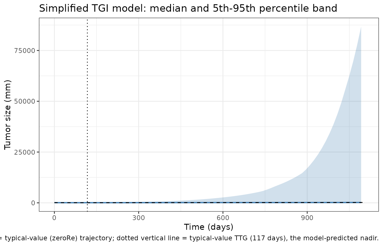
The characteristic shape is reproduced: shrinkage while the drug term dominates, a nadir at TTG, then regrowth as resistance takes over.
Derived TS metrics versus the published distributions
Claret 2014 reports the distributions of both TS metrics computed from individual empirical-Bayes (EBE) estimates. These are the model’s primary validation targets, and reproducing them is what identified the transposition of KDE and lambda in Supplementary Table S1 (see the dedicated section below, and Errata item 1). With that correction applied, both metrics fall where the paper puts them.
per_subject <- sim |> dplyr::filter(time == 0)
ts_w8   <- sim |> dplyr::filter(time == 56)  |> dplyr::pull(tumor_size)
ts_base <- sim |> dplyr::filter(time == 0)   |> dplyr::pull(tumor_size)
tsratio <- ts_w8 / ts_base

metric_tbl <- tibble::tibble(
  Metric = c("TTG (days)", "TSratio (week 8 / baseline)"),
  `Simulated median` = c(
    round(median(per_subject$ttg), 1),
    round(median(tsratio), 2)
  ),
  `Simulated 2.5-97.5%` = c(
    paste(round(quantile(per_subject$ttg, c(0.025, 0.975)), 0), collapse = " to "),
    paste(round(quantile(tsratio, c(0.025, 0.975)), 2), collapse = " to ")
  ),
  `Published, motesanib arm` = c("125 (28 to 399)", "0.69 (0.24 to 0.99)"),
  `Published, placebo arm`   = c("93 (-6 to 312)",  "0.77 (0.27 to 1.25)")
)
knitr::kable(metric_tbl)| Metric | Simulated median | Simulated 2.5-97.5% | Published, motesanib arm | Published, placebo arm |
|---|---|---|---|---|
| TTG (days) | 107.40 | 1 to 571 | 125 (28 to 399) | 93 (-6 to 312) |
| TSratio (week 8 / baseline) | 0.77 | 0.29 to 1.19 | 0.69 (0.24 to 0.99) | 0.77 (0.27 to 1.25) |
The tightest available check is on the typical value – all etas zero – because the TS model is a single pooled fit with no treatment-arm term. Its typical subject is therefore the pooled-cohort central subject, and its metrics must land between the two published per-arm medians. That statement involves no random draw at all, so it is asserted exactly.
ttg_typ     <- (log(KDE) - log(KL)) / LAM
tsratio_typ <- exp(KL * 56 - (KDE / LAM) * (1 - exp(-LAM * 56)))

c(TTG_typical = round(ttg_typ, 1), TSratio_typical = round(tsratio_typ, 3))
#>     TTG_typical TSratio_typical
#>         117.300           0.746

stopifnot(
  # Published per-arm medians: TTG 93 (placebo) and 125 (motesanib) days.
  ttg_typ > 93, ttg_typ < 125,
  # Published per-arm medians: TSratio 0.69 (motesanib) and 0.77 (placebo).
  tsratio_typ > 0.69, tsratio_typ < 0.77
)
Both typical values sit inside the published arm interval, which is what a pooled no-arm-term fit is supposed to do.
The cohort medians agree too, but they are asserted much more loosely: TTG is a ratio of log-normal quantities and is heavy-tailed, so a 200-subject median carries real sampling noise and its upper quantiles are not reproducible across rxode2 builds. The upper tail is deliberately not asserted on – a forward draw from a diagonal prior is also genuinely wider than a distribution of shrunken EBEs, so the published 97.5th percentiles are expected to be narrower than the simulated ones.
stopifnot(
  # Centre: within 40% of the published pooled median (~108 days). A
  # mis-transcribed rate constant moves this by 2- to 3-fold.
  abs(median(per_subject$ttg) / 108 - 1) < 0.4,
  # TTG is positive for the large majority of subjects, as reported (the
  # published placebo 2.5th percentile is -6 days, i.e. ~2.5% negative).
  # The closed-form probability is pnorm(log(KDE/KL)/sqrt(varKDE+varKL)) =
  # 0.952, so at n = 200 the binomial SE is 0.015; the bound is set ~7 SE
  # below it rather than the ~3 SE that 0.9 would give, because the eta draw
  # is not reproducible across rxode2 versions. This is a sanity check on the
  # sign of the drug effect, not a discriminator for the Table S1 erratum --
  # the printed reading would give a HIGHER positive fraction (0.983).
  mean(per_subject$ttg > 0) > 0.85,
  # Week-8 TSratio: net shrinkage, centred on the published 0.69-0.77.
  median(tsratio) < 1,
  abs(median(tsratio) / 0.73 - 1) < 0.25
)
How often is log(TTG + 100) undefined?
TTG is negative whenever KL > KDE, and the published shifted log
is undefined for TTG <= -100 days. No guard is added because none is
published. The exact probability under the Supplementary Table S1 IIV is
available in closed form – TTG = N / lambda with
N ~ Normal(log(KDE) - log(KL), sqrt(var_KDE + var_KL)) and
lambda log-normal – so it is integrated rather than
estimated by Monte Carlo:
mu_N    <- log(KDE) - log(KL)          # KDE/KL with the corrected assignment
sd_N    <- sqrt(0.679^2 + 1.18^2)      # SDs stay on their printed Table S1 rows
mu_lam  <- log(LAM)
sd_lam  <- 0.797

p_undefined <- integrate(
  function(lam) pnorm((-100 * lam - mu_N) / sd_N) * dlnorm(lam, mu_lam, sd_lam),
  lower = 0, upper = Inf
)$value

round(p_undefined, 5)
#> [1] 0.00454
stopifnot(p_undefined < 0.02)
About 0.5% of subjects drawn from the published IIV fall outside the
domain of log(TTG + 100) and return non-finite survival
quantities. Filter them explicitly in downstream work; the observed
MONET1 TTG range (-6 to 399 days) is comfortably inside the domain.
The OS model: covariate effects
On the AFT log-time scale every covariate is a multiplicative shift of median survival, so the following are exact identities that pin each Table 3 estimate.
os_grid <- expand.grid(RACE_ASIAN = c(0, 1), SMOKE_NEVER = c(0, 1)) |>
  dplyr::mutate(id = dplyr::row_number())

os_ev <- os_grid |>
  tidyr::expand_grid(time = c(0, 365)) |>
  dplyr::mutate(cmt = "tumor_size", evid = 0L, amt = NA_real_)

# Select only the outputs before joining: rxSolve echoes the covariate
# columns back, so joining os_grid without this select would silently
# produce RACE_ASIAN.x / RACE_ASIAN.y and leave $RACE_ASIAN NULL.
os_sim <- as.data.frame(
  rxode2::rxSolve(rxode2::zeroRe(tso), os_ev, returnType = "data.frame")
) |>
  dplyr::distinct(id, .keep_all = TRUE) |>
  dplyr::select(id, median_os, mu_os_logdays) |>
  dplyr::left_join(os_grid, by = "id")
#> ℹ omega/sigma items treated as zero: 'etalrbase', 'etalkge', 'etalkdrug', 'etallambda'
#> Warning: multi-subject simulation without without 'omega'

ref   <- os_sim$median_os[os_sim$RACE_ASIAN == 0 & os_sim$SMOKE_NEVER == 0]
asian <- os_sim$median_os[os_sim$RACE_ASIAN == 1 & os_sim$SMOKE_NEVER == 0]
never <- os_sim$median_os[os_sim$RACE_ASIAN == 0 & os_sim$SMOKE_NEVER == 1]

# Guard against an empty subset: `stopifnot()` passes vacuously on
# logical(0), so the length checks below are what make the ratio
# assertions meaningful.
stopifnot(length(ref) == 1L, length(asian) == 1L, length(never) == 1L)

knitr::kable(
  tibble::tibble(
    Contrast = c("Asian vs non-Asian", "Never- vs ever-smoker",
                 "Per +100 mm baseline TS"),
    `Model ratio` = c(asian / ref, never / ref, exp(-0.00197 * 100)),
    `Table 3 expectation` = c(exp(0.319), exp(0.264), exp(-0.197))
  ),
  digits = 4
)| Contrast | Model ratio | Table 3 expectation |
|---|---|---|
| Asian vs non-Asian | 1.3758 | 1.3758 |
| Never- vs ever-smoker | 1.3021 | 1.3021 |
| Per +100 mm baseline TS | 0.8212 | 0.8212 |
Both signs match the paper’s prose: survival probability is higher in Asian patients and lower in former and current smokers.
Figure 1: survival by TTG
Figure 1 of Claret 2014 splits the observed Kaplan-Meier curves by quartile of TTG. The quartile boundaries themselves are not published, so rather than invent midpoints the model analogue below is drawn at the TTG values the paper does print: the per-arm median and 2.5th/97.5th percentiles of the empirical-Bayes TTG distribution (Results, “TS model”).
mu_os <- function(ttg, tumsz = 90, asian = 0, ever = 1) {
  1.079 - 0.00197 * tumsz + 0.97695 * log(ttg + 100) +
    0.319 * asian - 0.264 * ever
}
sigma_os_aft <- exp(-0.24)

ttg_landmarks <- c(
  "2.5th pct, placebo (-6 d)"      = -6,
  "median, placebo (93 d)"         = 93,
  "median, motesanib (125 d)"      = 125,
  "97.5th pct, motesanib (399 d)"  = 399
)

km <- tidyr::expand_grid(
  landmark = factor(names(ttg_landmarks), levels = names(ttg_landmarks)),
  time     = seq(1, 1200, by = 5)
) |>
  dplyr::mutate(
    ttg = unname(ttg_landmarks[as.character(landmark)]),
    sur = 1 - pnorm((log(time) - mu_os(ttg)) / sigma_os_aft)
  )

ggplot(km, aes(time, sur, linetype = landmark)) +
  geom_line(linewidth = 0.7) +
  coord_cartesian(ylim = c(0, 1)) +
  labs(x = "Time (days)", y = "Survival probability", linetype = NULL,
       title = "Model-predicted survival across the published TTG range",
       caption = paste(
         "Reference subject: baseline TS 90 mm, non-Asian, ever-smoker.",
         "Compare Figure 1 of Claret 2014."
       )) +
  theme_bw()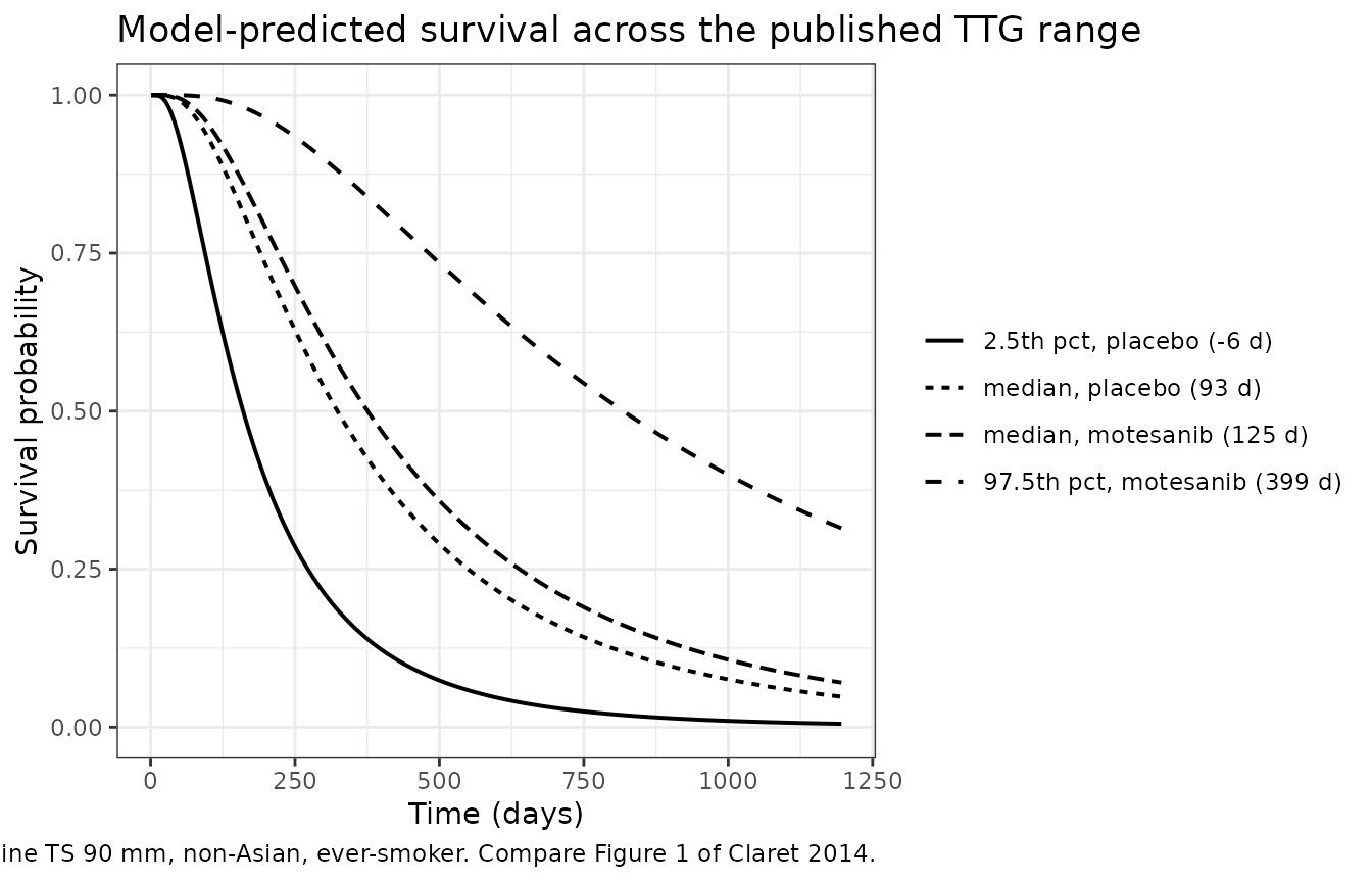
land_tbl <- tibble::tibble(
  `Published TTG landmark`           = names(ttg_landmarks),
  `TTG (days)`                       = unname(ttg_landmarks),
  `Median OS, ever-smoker (days)`    = round(exp(mu_os(unname(ttg_landmarks)))),
  `Median OS, never-smoker (days)`   = round(exp(mu_os(unname(ttg_landmarks), ever = 0)))
)
knitr::kable(land_tbl)| Published TTG landmark | TTG (days) | Median OS, ever-smoker (days) | Median OS, never-smoker (days) |
|---|---|---|---|
| 2.5th pct, placebo (-6 d) | -6 | 160 | 209 |
| median, placebo (93 d) | 93 | 323 | 421 |
| median, motesanib (125 d) | 125 | 376 | 489 |
| 97.5th pct, motesanib (399 d) | 399 | 818 | 1065 |
Across the published TTG range the model’s median survival for this reference subject spans roughly 160 days (2.5th percentile, ever-smoker) to 1,070 days (97.5th percentile, never-smoker). Figure 1’s four observed quartile curves cross S(t) = 0.5 in increasing order of TTG quartile, the first at roughly 200 days and the fourth somewhere between 600 and 800 days. No more precise reading is quoted here: the second- and third-quartile curves cross each other close to S(t) = 0.5, so their individual crossing times cannot be separated reliably from the printed figure. What survives that uncertainty is that the four medians are monotone in TTG quartile and lie inside the model’s span, which is the most that can be claimed.
Two reasons that comparison is qualitative only, and why nothing here is asserted on it. First, a digitized curve is evidence about the printed figure, not about the underlying patient data. Second, and more fundamentally, the two are not like-for-like: Figure 1’s curves pool all evaluable patients within a TTG quartile, mixing ethnicity, smoking history and baseline tumor size, whereas the model line is a single reference subject (90 mm, non-Asian, ever-smoker) at a TTG percentile rather than a quartile midpoint. The paper does not publish the quartile boundaries, so the two cannot be aligned.
The assertions below are therefore restricted to the two claims that are exact properties of Table 3: survival increases monotonically with TTG – the paper’s central claim – and never-smokers outlive ever-smokers at equal TTG.
Supplementary Table S1 transposes KDE and lambda
This is the one substantive correction this extraction makes to the published material, so the evidence is laid out in full.
Supplementary Table S1 prints, in this row order:
| Parameter | Estimate | RSE, % | SD |
|---|---|---|---|
| KL (day^-1) | 0.00107 | 7.70 | 1.18 |
| KDE (day^-1) | 0.0193 | 5.16 | 0.679 |
| lambda (day^-1) | 0.0103 | 3.72 | 0.797 |
| BASE (mm) | 90 | 2.37 | 0.683 |
| Sigma (mm) | 7.849 | 1.18 |
Read literally, that parameter set contradicts the paper’s own Results in two places at once, and by a wide margin. The model files therefore exchange the two bolded estimates, using KDE = 0.0103 and lambda = 0.0193 per day. Both numbers are taken verbatim from Table S1; only their row assignment changes, and no value is tuned to a target.
The decisive test does not involve the random effects
The TS model is a single pooled fit with no treatment-arm term. Its typical subject – every eta set to zero – is therefore the central subject of the pooled cohort, and its metrics must fall between the two published per-arm medians. No covariance structure, eta correlation or empirical-Bayes shrinkage argument can bear on this, because the typical value contains no etas at all.
typ_metrics <- function(kde, lam, kl = 0.00107, t8 = 56) {
  c(TTG = (log(kde) - log(kl)) / lam,
    TSratio = exp(kl * t8 - (kde / lam) * (1 - exp(-lam * t8))))
}

decisive <- rbind(
  `as printed in Table S1` = typ_metrics(0.0193, 0.0103),
  `corrected (this model)` = typ_metrics(0.0103, 0.0193)
)

knitr::kable(
  tibble::tibble(
    Reading = rownames(decisive),
    `Typical TTG (days)` = round(decisive[, "TTG"], 1),
    `Published arm medians` = "93 to 125",
    `Typical TSratio` = round(decisive[, "TSratio"], 3),
    `Published arm medians ` = "0.69 to 0.77"
  )
)| Reading | Typical TTG (days) | Published arm medians | Typical TSratio | Published arm medians |
|---|---|---|---|---|
| as printed in Table S1 | 280.8 | 93 to 125 | 0.467 | 0.69 to 0.77 |
| corrected (this model) | 117.3 | 93 to 125 | 0.746 | 0.69 to 0.77 |
stopifnot(
  # The printed reading falls outside BOTH published intervals.
  decisive["as printed in Table S1", "TTG"] > 125,
  decisive["as printed in Table S1", "TSratio"] < 0.69,
  # The corrected reading falls inside BOTH.
  decisive["corrected (this model)", "TTG"] > 93,
  decisive["corrected (this model)", "TTG"] < 125,
  decisive["corrected (this model)", "TSratio"] > 0.69,
  decisive["corrected (this model)", "TSratio"] < 0.77
)
The printed reading implies a typical patient who shrinks 53% by week 8 and does not reach nadir until day 281. The paper reports median shrinkage of 23% and 31% by arm and median nadir at days 93 and 125. That gap is far too large to be a shrinkage artefact, and – being eta-free – it cannot be one.
Two further published outputs agree independently
The forward Monte Carlo over the Table S1 IIV. This is a distributional check rather than a point one, and it discriminates on the lower tail as well as the centre. It is run in plain R rather than off the 200-subject rxode2 cohort so that it is reproducible across rxode2 builds.
set.seed(20140311)
n_mc <- 2e5
mc_metrics <- function(kde, lam) {
  kl_i  <- 0.00107 * exp(rnorm(n_mc, 0, 1.18))
  kde_i <- kde     * exp(rnorm(n_mc, 0, 0.679))
  lam_i <- lam     * exp(rnorm(n_mc, 0, 0.797))
  ttg_i <- (log(kde_i) - log(kl_i)) / lam_i
  tsr_i <- exp(kl_i * 56 - (kde_i / lam_i) * (1 - exp(-lam_i * 56)))
  c(ttg_med = median(ttg_i),
    tsr_med = median(tsr_i),
    tsr_p025 = unname(quantile(tsr_i, 0.025)))
}

mc <- rbind(`as printed` = mc_metrics(0.0193, 0.0103),
            `corrected`  = mc_metrics(0.0103, 0.0193))

knitr::kable(
  tibble::tibble(
    Reading = c(rownames(mc), "published (pooled)"),
    `Median TTG (days)` = c(round(mc[, "ttg_med"]), 108),
    `Median TSratio` = c(round(mc[, "tsr_med"], 2), 0.73),
    `TSratio 2.5th pct` = c(round(mc[, "tsr_p025"], 3), 0.25)
  )
)| Reading | Median TTG (days) | Median TSratio | TSratio 2.5th pct |
|---|---|---|---|
| as printed | 256 | 0.51 | 0.049 |
| corrected | 104 | 0.79 | 0.269 |
| published (pooled) | 108 | 0.73 | 0.250 |
s1_ttg_md <- unname(mc["corrected", "ttg_med"])

stopifnot(
  # The corrected median TTG is within 40% of the published pooled ~108 days;
  # the printed one is more than double it.
  abs(mc["corrected", "ttg_med"] / 108 - 1) < 0.4,
  mc["as printed", "ttg_med"] > 2 * 108,
  # The published TSratio 2.5th percentile is 0.24-0.27 by arm. The corrected
  # reading lands in that neighbourhood; the printed one is ~5-fold below it.
  mc["corrected", "tsr_p025"] > 0.2,
  mc["as printed", "tsr_p025"] < 0.1
)
The Table 5 simulation output, inverted through the Table 3 regression. Table 5 reports the paper’s own simulated median OS for a virtual phase III study in Asian patients: 594 days on CP + motesanib and 450 days on CP + placebo. Those numbers are outputs of the same Table 3 regression, so the regression can be inverted to recover the arm-level TTG the authors must have been conditioning on. This uses only published values – no digitization, no reconstructed quartiles.
invert_ttg <- function(median_os_days, tumsz = 90, asian = 1, ever = 1) {
  intercept <- 1.079 - 0.00197 * tumsz + 0.319 * asian - 0.264 * ever
  exp((log(median_os_days) - intercept) / 0.97695) - 100
}

tbl5_os   <- c(motesanib = 594, placebo = 450)
implied   <- invert_ttg(tbl5_os)
published <- c(motesanib = 125, placebo = 93)

knitr::kable(
  tibble::tibble(
    Arm = c("CP + motesanib", "CP + placebo"),
    `Table 5 simulated median OS (days)`  = unname(tbl5_os),
    `Implied TTG, ever-smoker (days)`     = round(unname(implied)),
    `Implied TTG, never-smoker (days)`    = round(unname(invert_ttg(tbl5_os, ever = 0))),
    `Published median TTG (days)`         = unname(published)
  )
)| Arm | Table 5 simulated median OS (days) | Implied TTG, ever-smoker (days) | Implied TTG, never-smoker (days) | Published median TTG (days) |
|---|---|---|---|---|
| CP + motesanib | 594 | 159 | 98 | 125 |
| CP + placebo | 450 | 95 | 49 | 93 |
Inverting Table 5 recovers arm-level TTGs in the same 90-160 day band as the Results-text medians, and feeding the Results-text medians forward through the Table 3 regression recovers Table 5’s survival times – 445 days computed against 450 published on placebo. The printed Table S1 TTG of 281 days instead implies a median OS of 864 days: 1.5 times Table 5’s motesanib arm (594 days), 1.9 times its placebo arm (450 days), and 1.8 times the 479 days implied by the published pooled TTG of about 108 days. That last ratio is the like-for-like one – 281 and 108 days are both pooled typical values – and it is the comparison asserted on below.
forward_os <- function(ttg, tumsz = 90, asian = 1, ever = 1) {
  exp(1.079 - 0.00197 * tumsz + 0.97695 * log(ttg + 100) +
        0.319 * asian - 0.264 * ever)
}

knitr::kable(
  tibble::tibble(
    `TTG source` = c("Results text, placebo (93 d)",
                     "Results text, motesanib (125 d)",
                     "Table S1 as printed, typical (281 d)",
                     "Table S1 corrected, typical (117 d)"),
    `Median OS via Table 3 (days)` = round(forward_os(c(93, 125, 280.8, 117.3))),
    `Table 5 published (days)` = c(450, 594, NA, NA)
  )
)| TTG source | Median OS via Table 3 (days) | Table 5 published (days) |
|---|---|---|
| Results text, placebo (93 d) | 445 | 450 |
| Results text, motesanib (125 d) | 517 | 594 |
| Table S1 as printed, typical (281 d) | 864 | NA |
| Table S1 corrected, typical (117 d) | 500 | NA |
stopifnot(
  # Table 5 inverts to a longer TTG on motesanib than on placebo: the drug effect.
  implied["motesanib"] > implied["placebo"],
  # Table 5 and the Results-text medians agree within 50% on both arms.
  all(abs(implied / published - 1) < 0.5),
  # The published placebo TTG reproduces Table 5's placebo arm closely.
  abs(forward_os(93) / 450 - 1) < 0.1,
  # The printed Table S1 typical TTG overshoots even the BETTER of the two
  # published Table 5 arms by more than 40%.
  forward_os(280.8) > 1.4 * 594,
  # Like-for-like: both 280.8 d and 108 d are pooled/typical TTG values, so
  # this is the comparison the transposition actually distorts -- by >70%.
  forward_os(280.8) / forward_os(108) > 1.7,
  # The corrected typical TTG lands inside the published arm range.
  forward_os(117.3) > 450, forward_os(117.3) < 594
)
Why a transposition, and why not something else
Four independent published quantities – the Results-text TTG medians, the Results-text TSratio medians and percentiles, the Table 3 regression and the Table 5 simulation output – all place the operative TTG scale near 100 days and the week-8 TSratio near 0.73. Exchanging the two Table S1 estimates reproduces every one of them; leaving them as printed misses each by 2- to 5-fold.
A transposition of two adjacent rows is also the most economical explanation. Both candidate values already appear in the table, so nothing is invented, and a swap moves both metrics coherently – which a single mistyped digit would not, since TTG and TSratio each depend on KDE and lambda together.
The competing explanation, that a forward draw from a diagonal prior is simply the wrong comparator for a median of correlated empirical-Bayes estimates, is ruled out by the decisive test above: it is an argument about the distribution of etas, and the typical value has none.
One sub-choice is genuinely undetermined and is not load-bearing. The estimates alone may be transposed (the reading used here: KDE keeps the printed KDE row’s RSE and SD), or the whole rows including labels may be swapped. The two differ by about one day in median TTG (104 vs 105). The estimate-only reading is preferred because it matches the published lower tails slightly better – a TSratio 2.5th percentile of 0.269 against 0.196, versus a published 0.24-0.27.
This has been recorded for author correspondence; until the authors
confirm, users who need to reproduce the paper’s printed Table
S1 exactly can override the two values with
rxode2::ini().
The nonevaluable-patient model
For the 14% of patients with no predictable TS metric, survival depends only on baseline serum albumin.
alb_grid <- data.frame(id = 1:5, time = 365, ALB = c(25, 30, 35, 40, 45))
nev_sim  <- as.data.frame(rxode2::rxSolve(nev, alb_grid, returnType = "data.frame"))

knitr::kable(
  nev_sim |>
    dplyr::select(ALB, median_os, sur) |>
    dplyr::rename(
      "Baseline albumin (g/L)" = ALB,
      "Median OS (days)" = median_os,
      "S(365 days)" = sur
    ),
  digits = c(0, 1, 3)
)| Baseline albumin (g/L) | Median OS (days) | S(365 days) |
|---|---|---|
| 25 | 29.4 | 0.064 |
| 30 | 50.5 | 0.115 |
| 35 | 86.6 | 0.192 |
| 40 | 148.6 | 0.293 |
| 45 | 254.9 | 0.414 |
# Exact identity: +10 g/L albumin multiplies median OS by exp(10 * 0.108).
ratio_10 <- nev_sim$median_os[nev_sim$ALB == 45] / nev_sim$median_os[nev_sim$ALB == 35]
stopifnot(
  length(ratio_10) == 1L,
  abs(ratio_10 - exp(1.08)) < 1e-8,
  max(abs(nev_sim$sur - exp(-nev_sim$cumhazard))) < 1e-12
)
The albumin coefficient’s units are self-checking. At a typical 38 g/L the model gives a median OS of
exp(0.681 + 0.108 * 38)
#> [1] 119.7014
days – a poor outcome, consistent with patients who never had an evaluable postbaseline scan. Reading the same coefficient as “per g/dL” would give
exp(0.681 + 0.108 * 3.8)
#> [1] 2.978441
days, which is impossible. Supplementary Table S2 labels the row “Baseline albumin (g/L)”, and the arithmetic confirms it.
An external check on the absolute scale (Supplementary Figure S3)
Supplementary Figure S3 is the paper’s own visual predictive check for this model: observed Kaplan-Meier curves for the nonevaluable patients in each arm, overlaid with the model’s prediction band. Locating the axis tick marks in the figure and interpolating between them, the motesanib curve crosses S(t) = 0.5 at about 70 days and the placebo curve at about 125 days (the placebo step sits flat on 0.5 from about 117 to 129 days, which sets the resolution of the reading). Digitizing a printed step function is evidence about the figure, not about the underlying data, so nothing below is asserted on those numbers tightly – the assertions are stated with enough margin to absorb a +/- 25% reading error.
What is robust to that reading error is the scale. Serum albumin in advanced-cancer patients runs roughly 30-45 g/L. Under the labelled g/L reading that range brackets both digitized medians; under a g/dL misreading the model misses by a factor of about fifty, which no plausible digitizing error can close.
med_os_alb <- function(alb) exp(0.681 + 0.108 * alb)

scale_tbl <- tibble::tibble(
  Reading = c("g/L (as labelled)", "g/dL (the misreading)"),
  `Plausible albumin range` = c("30 to 45 g/L", "3.0 to 4.5 g/dL"),
  `Model median OS (days)` = c(
    paste(round(med_os_alb(c(30, 45))), collapse = " to "),
    paste(round(med_os_alb(c(3.0, 4.5)), 1), collapse = " to ")
  ),
  `At a typical 40 g/L (4.0 g/dL)` = round(med_os_alb(c(40, 4.0)), 1)
)
knitr::kable(scale_tbl)| Reading | Plausible albumin range | Model median OS (days) | At a typical 40 g/L (4.0 g/dL) |
|---|---|---|---|
| g/L (as labelled) | 30 to 45 g/L | 50 to 255 | 148.6 |
| g/dL (the misreading) | 3.0 to 4.5 g/dL | 2.7 to 3.2 | 3.0 |
stopifnot(
  # Across the plausible albumin range the g/L reading brackets both digitized
  # per-arm medians (about 70 days motesanib, 125 days placebo), with margin on
  # both sides rather than a bound that tracks the point estimate.
  med_os_alb(30) < 70, med_os_alb(45) > 125,
  # The g/dL reading is ~50-fold too low -- not a borderline call.
  med_os_alb(4.0) < 5
)
The albumin imbalance the paper invokes is also the right size: inverting the regression at the two digitized medians implies
implied_alb <- (log(c(motesanib = 70, placebo = 125)) - 0.681) / 0.108
round(implied_alb, 1)
#> motesanib   placebo
#>      33.0      38.4

stopifnot(
  # Both implied values land inside the physiologic albumin range, so the g/L
  # reading is self-consistent. A +/- 25% error on either digitized median
  # moves the implied albumin by only about 2.7 g/L, well inside this window.
  all(implied_alb > 25), all(implied_alb < 50),
  # The paper's own explanation: the placebo arm did better because its
  # nonevaluable patients started with HIGHER baseline albumin.
  implied_alb[["placebo"]] > implied_alb[["motesanib"]]
)
g/L, i.e. an arm difference of about 5.4 g/L – a modest, entirely plausible baseline imbalance, which is precisely the explanation Claret 2014 offers for the better outcome in the placebo arm among these patients. Under the g/dL misreading the same two medians would demand baseline albumins of 33 and 38.4 g/dL, roughly eight-fold above any physiologic value.
nev_curves <- tidyr::expand_grid(
  ALB = c(25, 30, 35, 40, 45),
  time = seq(1, 1200, by = 5)
) |>
  dplyr::mutate(
    sur = 1 - pnorm((log(time) - (0.681 + 0.108 * ALB)) / exp(0.502)),
    Albumin = factor(paste(ALB, "g/L"), levels = paste(c(25, 30, 35, 40, 45), "g/L"))
  )

ggplot(nev_curves, aes(time, sur, colour = Albumin)) +
  geom_line(linewidth = 0.7) +
  coord_cartesian(ylim = c(0, 1)) +
  labs(x = "Time (days)", y = "Survival probability",
       title = "Nonevaluable patients: survival by baseline albumin",
       caption = paste(
         "Compare Supplementary Figure S3 of Claret 2014, the paper's visual",
         "predictive check for this model against the observed per-arm",
         "Kaplan-Meier curves.")) +
  theme_bw()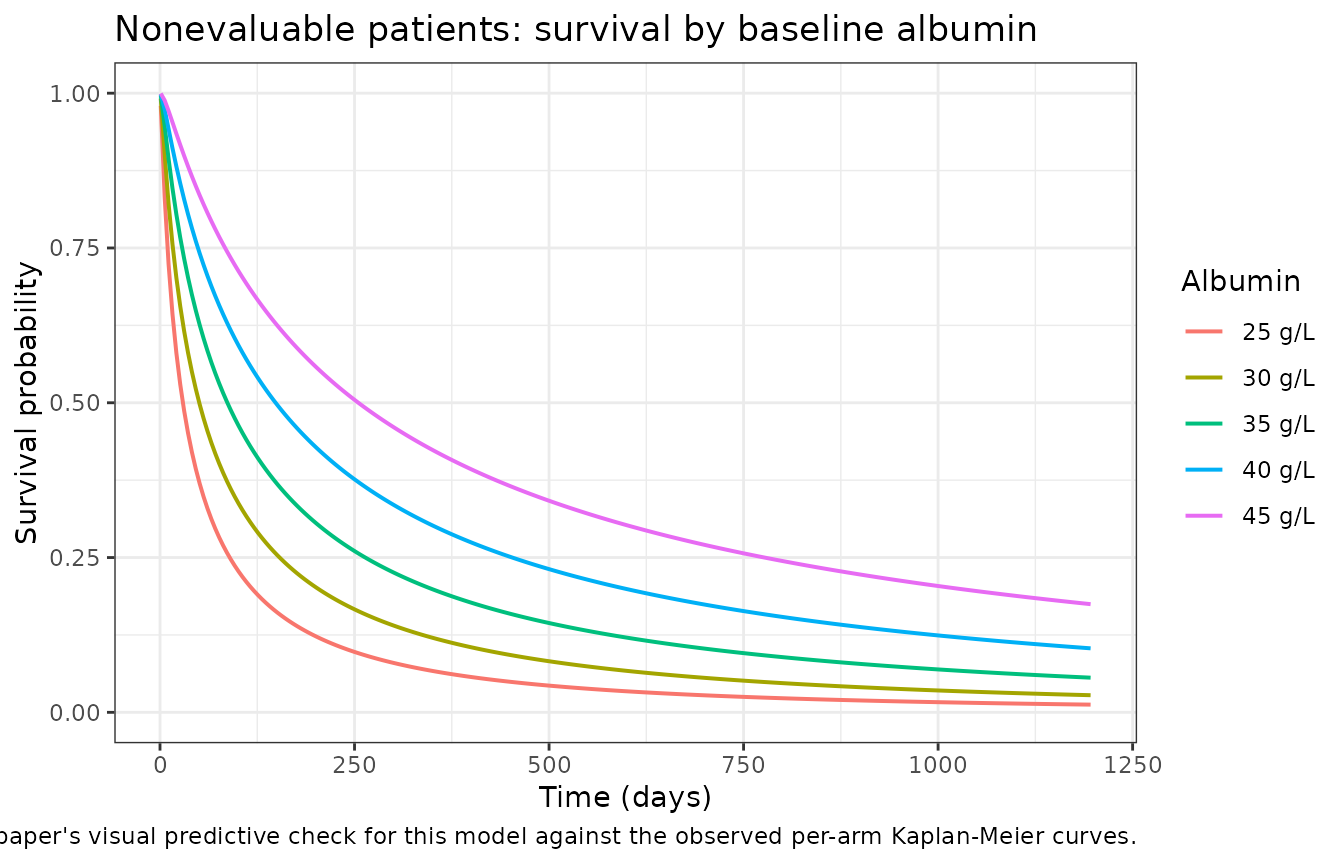
This reproduces the paper’s observation that an imbalance in baseline albumin could account for the better outcome seen in the CP-plus-placebo arm than in the CP-plus-motesanib arm among nonevaluable patients.
Why no NCA
Neither model contains a pharmacokinetic compartment. The simplified
TGI model is explicitly not exposure-driven – motesanib’s 125
mg once-daily regimen enters only through the estimated
kdrug and lambda – and the OS models consume
covariates, not concentrations. There is therefore no concentration-time
profile to run through PKNCA. Validation here is by structural identity
and by comparison against the paper’s published figures and tables,
following the same pattern as
vignette("Struemper_2025_tumorsize_OS_nsclc") and
vignette("Nagy_2017_obiltoxaximab").
Assumptions and deviations
-
Supplementary Table S1 transposes the KDE and lambda estimates; this extraction exchanges them. Table S1 prints KDE = 0.0193 and lambda = 0.0103 per day; the model file uses KDE = 0.0103 and lambda = 0.0193. Both numbers are verbatim from Table S1 – only their row assignment changes, and no value is tuned toward any target. The full argument, with assertions, is in the section “Supplementary Table S1 transposes KDE and lambda” above. In brief:
- The decisive test is eta-free. The TS model is a single pooled fit with no treatment-arm term, so its typical value must lie between the two published per-arm medians. As printed it gives a typical TTG of 281 days and a week-8 TSratio of 0.467, outside the published 93-125 day and 0.69-0.77 intervals on both counts; corrected it gives 117 days and 0.746, inside both. Because the typical value contains no random effects, no eta-correlation or empirical-Bayes-shrinkage argument can account for the gap.
- Forward Monte Carlo over the Table S1 IIV corroborates on the lower tail: the corrected reading gives a median TTG of 104 days and a TSratio 2.5th percentile near 0.27 against a published 0.24-0.27, while the printed reading gives 257 days and 0.05.
- Feeding the published TTG medians forward through the Table 3 regression reproduces Table 5’s simulated survival (445 days computed vs 450 published on placebo); the printed Table S1 TTG implies roughly 865 days.
A prior draft of this vignette attributed the same discrepancy to the difference between a forward marginal draw and a distribution of correlated empirical-Bayes estimates, and left Table S1 unchanged. The eta-free typical- value test above rules that explanation out.
This has not been confirmed with the authors and no erratum to the paper is known. Users who need the printed Table S1 values can restore them with
rxode2::ini(), at the cost of no longer matching the paper’s Results. The TS sub-model has no treatment-arm term. It is a single pooled fit across both MONET1 arms, so a forward simulation with freshly drawn etas produces the same TS and TTG distribution for motesanib and placebo. The paper’s arm difference arises entirely from the individual empirical-Bayes estimates, and its trial simulations “were conditioned on ‘predicted’ tumor reductions and patient characteristics of MONET1 data”. Consequently the packaged model cannot generate the published hazard ratios (Table 4: 0.88 full population, 0.76 Asian) or the Table 5 power calculations de novo – those require the individual-level MONET1 data, which are not public. Neither is asserted in this vignette.
IIV scale. Supplementary Table S1’s fourth column is headed “SD” and its abbreviation line defines it as the “standard deviation of inter-patient variability in diagonal covariance matrix”. The values are therefore squared to give the variances nlmixr2’s
eta ~ variancesyntax expects. This choice does not affect any median, so the checks in this vignette cannot discriminate it; the table’s own wording is the evidence.Smoking-history polarity. Table 3’s coefficient (-0.264) is defined for “former and current smokers as compared with those who had never smoked”, i.e. on an ever-smoker indicator. The canonical register column is
SMOKE_NEVER, somodel()forms the ever-smoker indicator as1 - SMOKE_NEVER. This keeps both the published intercept (1.079) and the published coefficient intact, preserving their correspondence with the Supplementary Table S3 covariance matrix; re-parameterising directly ontoSMOKE_NEVERwould have required shifting the intercept to 0.815.Baseline TS in the OS model. The paper’s OS regression uses observed baseline tumor size. The joint model uses the TS sub-model’s own individual
rbase, following the convention ofmodellib("Struemper_2025_tumorsize_OS_nsclc"). The two coincide at the typical value (90 mm) and differ only by estimation shrinkage.Nonevaluable cohort size. Supplementary Table S2 is titled “… for Non-evaluable Patients (n = 146)”, but the main text reports 156 nonevaluable patients (88 motesanib + 68 placebo, and separately 115 + 41). The paper does not reconcile the two; the most likely explanation is that 10 patients lacked a baseline albumin measurement.
population$n_subjectsis set to 146 (the number the regression was actually fitted on); the 14% correction applied in the simulations uses 156.Supplementary Figure S1 axis labels. The goodness-of-fit panels label both axes “(cm)”, but the Methods, Table S1 and the plotted range (0-420 with a typical baseline of 90) are all mm. Treated as a figure-labelling error; the models use mm throughout.
log(TTG + 100)is left unguarded. The published model is undefined for TTG <= -100 days and the paper specifies no fallback, so none is invented. The probability is quantified above (about 0.5% under the published IIV) rather than silently clipped.No IIV or residual error on either OS model. Neither Table 3 nor Supplementary Table S2 reports any; the AFT scale parameter is the sole source of between-subject survival variability. No etas are invented.
The historical OS model is not extracted. Claret 2014 evaluates the earlier first-line NSCLC OS model of Wang et al. (its reference 7) but does not reprint its parameter estimates, so it cannot be sourced from this paper.
TTG time unit: the Methods say weeks, everything else says days. The Methods define metric 2 as “Time to tumor growth (TTG), the time to nadir TS (in weeks)”. Four other locations contradict that word: the Methods themselves state that “the parameters KL, KDE, and
lambdahave inverse of time units (e.g., day^-1)”, so(log(KDE) - log(KL)) / lambdais in days; Table 3 heads the rowLog(TTG*(day)); Table 3 footnote c states that survival time was analysed in days; and the Results report the TTG medians as “125 (28-399) vs. 93 (-6 to 312) days”. TTG is therefore taken as days throughout, as is the shift constant inlog(TTG + 100). Reading “(in weeks)” literally would rescale TTG by a factor of 7 and, through the 0.97695 coefficient onlog(TTG*), would move predicted median survival by a factor of roughly 6, so the distinction is load-bearing rather than cosmetic.Figure-digitized values are used for narrative only, never for parameters. Two numbers in this vignette were read off a printed figure rather than taken from the text or tables: the Supplementary Figure S3 per-arm median survival times for nonevaluable patients (about 70 days on motesanib and about 125 days on placebo). Both were obtained by locating the printed axis tick marks in the page image and interpolating linearly between them, not by eye. Figure 1’s TTG-quartile medians are deliberately not quoted numerically – the second- and third-quartile curves cross near S(t) = 0.5, so those two crossing times cannot be separated reliably from the printed figure, and only the monotone ordering is claimed. Every
ini()value in both model files comes from Table 3, Supplementary Table S1 or Supplementary Table S2; no parameter is derived from a figure. The assertions that reference the two digitized readings are stated as windows wide enough to absorb a +/- 25% reading error.