Week-8 disease control rate as a predictor of OS and PFS in NSCLC (Claret 2014)

Model and source

• Citation: Claret L, Gupta M, Han K, Joshi A, Sarapa N, He J, Powell B, Bruno R. Prediction of overall survival or progression free survival by disease control rate at week 8 is independent of ethnicity: Western versus Chinese patients with first-line non-small cell lung cancer treated with chemotherapy with or without bevacizumab. J Clin Pharmacol. 2014;54(3):253-257. doi:10.1002/jcph.191. Parameter estimates are from Table 2 (Parameter Estimates of the OS Model). The companion PFS model from the same paper (Table 3) is available as modellib(‘Claret_2014_DCR_PFS_nsclc’).
• Article: J Clin Pharmacol. 2014;54(3):253-257

This paper contributes two models to nlmixr2lib, matching the two independent survreg regressions the authors report:

• modellib("Claret_2014_DCR_OS_nsclc") – overall survival (paper Table 2).
• modellib("Claret_2014_DCR_PFS_nsclc") – progression-free survival (paper Table 3).

Both are accelerated failure time (AFT) log-normal survival regressions with no PK input, no ODE state, no inter-individual variability and no residual error. They are algebraic: given a patient’s covariates they return the location parameter of log(T), the median survival time, and the survivor function directly.

• OS description: Parametric overall-survival (OS) model for first-line advanced non-small cell lung cancer (NSCLC), linking the week-8 RECIST disease control rate (DCR) to survival. Accelerated failure time (AFT) log-normal regression fit with the R survreg function to pooled individual-level data from 774 evaluable patients in two bevacizumab-plus-chemotherapy studies: E4599 (Phase III, 878 Western patients, bevacizumab + carboplatin/paclitaxel versus carboplatin/paclitaxel) and SAiL (Phase IV single arm, 198 Chinese patients). The location parameter of log(OS) is a linear function of two retained binary covariates: week-8 disease control (CR + PR + SD versus PD) and baseline hypoalbuminaemia (< 3.5 g/dL). Bevacizumab treatment, Chinese ethnicity and ECOG performance status were all significant in univariate Cox screening but were eliminated in backward selection – disease control fully captured the bevacizumab effect on OS, so the authors describe the final OS model as drug independent. The model is algebraic and deterministic (no ODE state, no PK input, no IIV, no residual error): it returns the survivor function directly. The companion progression-free-survival model from the same paper is modellib(‘Claret_2014_DCR_PFS_nsclc’).
• PFS description: Parametric progression-free-survival (PFS) model for first-line advanced non-small cell lung cancer (NSCLC), linking the week-8 RECIST disease control rate (DCR) to PFS. Accelerated failure time (AFT) log-normal regression fit with the R survreg function to pooled individual-level data from 774 evaluable patients in two bevacizumab-plus-chemotherapy studies: E4599 (Phase III, 878 Western patients, bevacizumab + carboplatin/paclitaxel versus carboplatin/paclitaxel) and SAiL (Phase IV single arm, 198 Chinese patients). The location parameter of log(PFS) is a linear function of two retained binary covariates: week-8 disease control (CR + PR + SD versus PD) and bevacizumab treatment. Unlike the companion overall-survival model, disease control did NOT fully capture the bevacizumab effect here, so a separate bevacizumab term is retained and the authors state the PFS model cannot be assumed drug independent. Baseline albumin, ECOG performance status and Chinese ethnicity were all significant in univariate Cox screening but were eliminated in backward selection. The model is algebraic and deterministic (no ODE state, no PK input, no IIV, no residual error): it returns the survivor function directly. The companion overall-survival model from the same paper is modellib(‘Claret_2014_DCR_OS_nsclc’).

Population

The models were fit to the evaluable population of two bevacizumab studies in first-line advanced non-small cell lung cancer (NSCLC): the Phase III E4599 study in 878 Western patients (bevacizumab + carboplatin/paclitaxel versus carboplatin/paclitaxel alone) and the single-arm Phase IV SAiL study in 198 Chinese patients. To be evaluable a patient needed at least one response assessment between weeks 3 and 14, and the assessment closest to week 8 was the one used; 629 of 878 Western patients (72%) and 145 of 198 Chinese patients (73%) qualified, giving n = 774.

Patient characteristics were limited to two well-established prognostic factors: baseline serum albumin (< 3.5 g/dL versus >= 3.5 g/dL) and ECOG performance status (0 versus >= 1). Low albumin was much more common in the Western study (29%) than the Chinese one (6%), while ECOG >= 1 was slightly more common in the Chinese study (78% versus 60%).

Week-8 response categories in the evaluable population reproduce the paper’s Table 1:

table1 <- tibble::tribble(
  ~Study,    ~Arm,             ~CR, ~PR,  ~SD,  ~PD, ~Total,
  "Western", "Chemo",           2L,  67L, 152L,  99L,   320L,
  "Western", "Bev + Chemo",     4L, 133L, 128L,  44L,   309L,
  "Chinese", "Bev + Chemo",     2L,  67L,  69L,   7L,   145L
) |>
  dplyr::mutate(DCR = (CR + PR + SD) / Total)

stopifnot(with(table1, all(CR + PR + SD + PD == Total)))

table1 |>
  dplyr::mutate(DCR = sprintf("%.1f%%", 100 * DCR)) |>
  knitr::kable(caption = "Week-8 response categories in the evaluable population (reproduces Claret 2014 Table 1); DCR = (CR + PR + SD) / Total.")

Week-8 response categories in the evaluable population (reproduces Claret 2014 Table 1); DCR = (CR + PR + SD) / Total.

Study	Arm	CR	PR	SD	PD	Total	DCR
Western	Chemo	2	67	152	99	320	69.1%
Western	Bev + Chemo	4	133	128	44	309	85.8%
Chinese	Bev + Chemo	2	67	69	7	145	95.2%

The paper’s observation that disease control was higher in the Chinese study (95%) than among Western bevacizumab-treated patients (85%) is recovered exactly by the last column.

The same information is available programmatically from each model’s population metadata (mod_os$population).

Source trace

Every ini() value is carried with an in-file comment in inst/modeldb/therapeuticArea/oncology/Claret_2014_DCR_OS_nsclc.R and ..._PFS_nsclc.R. They are collected here for review.

Model	Parameter	Value	SE	Source location
OS	mu_os_int	1.855	0.0613	Table 2, row “Intercept”
OS	e_dcr_mu_os	0.939	0.0646	Table 2, row “DCR”
OS	e_alb_lt35_mu_os	-0.270	0.0601	Table 2, row “Albumin < 3.5 (g/dL)”
OS	lsigma_os	-0.370	0.0308	Table 2, row “Log (scale)”
PFS	mu_pfs_int	0.466	0.0477	Table 3, row “Intercept”
PFS	e_dcr_mu_pfs	1.378	0.0525	Table 3, row “DCR”
PFS	e_bev_mu_pfs	0.232	0.0429	Table 3, row “Bevacizumab”
PFS	lsigma_pfs	-0.641	0.0282	Table 3, row “Log (scale)”
both	AFT log-normal form, survreg	n/a		Methods, “Survival Model Development”; Results, “Overall Survival Model” and “PFS Model”
both	Week-8 DCR definition (CR + PR + SD vs PD)	n/a		Methods, “Response Metrics”
both	Albumin dichotomy at 3.5 g/dL; ECOG dichotomy at 1	n/a		Methods, “Patient Characteristics”
both	Censoring: study duration ~ Uniform(8, 30) months	n/a		Methods, “Survival Model Development”

Sign recovery for the negative coefficients

Three of the eight estimates are negative. Their minus signs are typeset as U+2212 and are dropped by both the trimmed-markdown conversion of the PDF and by pdftotext -layout, so they cannot be taken from a text extraction. They were recovered from the tables’ own Wald statistics – z equals estimate divided by SE on every row, so the sign of z supplies the sign of the estimate – and then confirmed by reading the rendered page image.

sign_check <- tibble::tribble(
  ~Model, ~Parameter,           ~Estimate, ~SE,     ~z_published,
  "OS",   "Intercept",            1.855,   0.0613,   30.2,
  "OS",   "DCR",                  0.939,   0.0646,   14.5,
  "OS",   "Albumin < 3.5 g/dL",  -0.270,   0.0601,   -4.5,
  "OS",   "Log (scale)",         -0.370,   0.0308,  -12.0,
  "PFS",  "Intercept",            0.466,   0.0477,    9.8,
  "PFS",  "DCR",                  1.378,   0.0525,   26.2,
  "PFS",  "Bevacizumab",          0.232,   0.0429,    5.4,
  "PFS",  "Log (scale)",         -0.641,   0.0282,  -22.7
) |>
  dplyr::mutate(z_recomputed = Estimate / SE,
                rel_diff = abs(z_recomputed / z_published - 1),
                agrees = sign(z_recomputed) == sign(z_published) & rel_diff < 0.01)

# Every row must reproduce the published Wald statistic, sign included.
#
# The test is stated relatively rather than absolutely because the published
# estimate, SE and z are each rounded: the largest honest disagreement across
# the eight rows is 0.31% (the intercept, 30.261 recomputed vs 30.2 printed),
# so a 1% tolerance absorbs rounding. It remains an extremely strict test of
# the signs -- a flipped sign changes z by twice its magnitude, i.e. a relative
# difference of 200%, which is 640-fold above the threshold and could not be
# mistaken for rounding.
stopifnot(all(sign_check$agrees), max(sign_check$rel_diff) < 0.01)

sign_check |>
  dplyr::mutate(z_recomputed = round(z_recomputed, 2),
                rel_diff = sprintf("%.2f%%", 100 * rel_diff)) |>
  dplyr::rename("Published z" = z_published, "Estimate / SE" = z_recomputed,
                "Relative difference" = rel_diff, "Signs agree" = agrees) |>
  knitr::kable(caption = "Sign recovery: estimate / SE reproduces the published Wald statistic for all eight parameters, which fixes the sign of each.")

Sign recovery: estimate / SE reproduces the published Wald statistic for all eight parameters, which fixes the sign of each.

Model	Parameter	Estimate	SE	Published z	Estimate / SE	Relative difference	Signs agree
OS	Intercept	1.855	0.0613	30.2	30.26	0.20%	TRUE
OS	DCR	0.939	0.0646	14.5	14.54	0.25%	TRUE
OS	Albumin < 3.5 g/dL	-0.270	0.0601	-4.5	-4.49	0.17%	TRUE
OS	Log (scale)	-0.370	0.0308	-12.0	-12.01	0.11%	TRUE
PFS	Intercept	0.466	0.0477	9.8	9.77	0.31%	TRUE
PFS	DCR	1.378	0.0525	26.2	26.25	0.18%	TRUE
PFS	Bevacizumab	0.232	0.0429	5.4	5.41	0.15%	TRUE
PFS	Log (scale)	-0.641	0.0282	-22.7	-22.73	0.13%	TRUE

The negative albumin coefficient is independently corroborated by the paper’s prose – “the probability to survive decreases in patients with low baseline albumin” – and the positive bevacizumab coefficient by “the probability of progression or death decreases in patients with disease control and with bevacizumab treatment”.

Mechanism in one paragraph

survreg’s log-normal fit is the AFT form log(T) = mu + sigma * eps with eps ~ N(0, 1), so T is log-normal with median exp(mu) and the table’s Log (scale) row is log(sigma). Each model makes mu linear in its retained binary covariates and leaves sigma covariate-free, which means every covariate acts as a pure multiplier on median survival: disease control at week 8 multiplies median OS by exp(0.939) = 2.56 and median PFS by exp(1.378) = 3.97; low albumin multiplies median OS by exp(-0.270) = 0.76; bevacizumab multiplies median PFS by exp(0.232) = 1.26. The survivor function is S(t) = 1 - Phi((log(t) - mu) / sigma).

The structural difference between the two models is the paper’s main result. In the OS model, bevacizumab treatment was significant univariately but dropped out of the multivariate model because week-8 disease control fully captured it, so the final OS model carries no drug term at all and the authors describe it as drug independent. In the PFS model, disease control did not fully capture the bevacizumab effect, so a separate DRUG_BEV term is retained. Chinese ethnicity was significant univariately for both endpoints and eliminated from both final models, with no DCR-by-ethnicity interaction – the paper’s title result.

Structural identities

Before comparing against anything published, check that the packaged models compute what the AFT algebra says they should. These are exact identities, so they are asserted tightly.

# The models are algebraic: a plain data frame of id / time / covariates is a
# valid event table. There are no ODE states, so there is no `cmt` and no
# `evid`, and no `omega = NA` (these models declare no etas at all).
grid_os <- tidyr::expand_grid(RESP_DCR = c(0, 1), ALB_LT35 = c(0, 1)) |>
  dplyr::mutate(id = dplyr::row_number()) |>
  tidyr::expand_grid(time = c(1, 3, 6, 12, 24, 36))

sim_os <- as.data.frame(rxode2::rxSolve(mod_os, events = grid_os,
                                        keep = c("RESP_DCR", "ALB_LT35")))

# 1. median_os is exactly exp(mu_os).
stopifnot(max(abs(sim_os$median_os - exp(sim_os$mu_os))) < 1e-10)

# 2. cumhazard_os is exactly -log(sur_os).
stopifnot(max(abs(sim_os$cumhazard_os + log(sim_os$sur_os))) < 1e-8)

# 3. sur_os matches the closed-form log-normal survivor function.
sur_closed <- 1 - pnorm((log(sim_os$time) - sim_os$mu_os) / sim_os$sigma_os)
stopifnot(max(abs(sim_os$sur_os - sur_closed)) < 1e-6)

# 4. Covariate effects are exact multipliers on the median. Compare the four
#    covariate cells by key, never by row position.
med <- sim_os |>
  dplyr::distinct(RESP_DCR, ALB_LT35, median_os)
cell <- function(d, a) {
  v <- med$median_os[med$RESP_DCR == d & med$ALB_LT35 == a]
  if (length(v) != 1L) stop("no unique cell for DCR=", d, " ALB=", a)
  v
}
stopifnot(
  abs(cell(1, 0) / cell(0, 0) - exp(0.939))  < 1e-8,   # DCR effect
  abs(cell(1, 1) / cell(1, 0) - exp(-0.270)) < 1e-8,   # albumin effect
  # The model is additive on the log scale, so the two effects must be
  # exactly multiplicative on the median with no interaction term.
  abs(cell(1, 1) / cell(0, 0) - exp(0.939 - 0.270)) < 1e-8
)

# 5. The survivor function at t = median must be exactly 0.5 -- a definitional
#    check that exercises the pnorm path against the mu/sigma path.
at_median <- med |>
  dplyr::mutate(id = dplyr::row_number(), time = median_os) |>
  dplyr::select(id, time, RESP_DCR, ALB_LT35)
sur_at_median <- as.data.frame(rxode2::rxSolve(mod_os, events = at_median))$sur_os
stopifnot(max(abs(sur_at_median - 0.5)) < 1e-6)

med |>
  dplyr::arrange(RESP_DCR, ALB_LT35) |>
  dplyr::mutate(median_os = round(median_os, 2)) |>
  dplyr::rename("Week-8 disease control" = RESP_DCR,
                "Albumin < 3.5 g/dL" = ALB_LT35,
                "Median OS (months)" = median_os) |>
  knitr::kable(caption = "Median overall survival by covariate cell. The 2.56-fold disease-control effect and 0.76-fold low-albumin effect are exact multipliers.")

Median overall survival by covariate cell. The 2.56-fold disease-control effect and 0.76-fold low-albumin effect are exact multipliers.

Week-8 disease control	Albumin < 3.5 g/dL	Median OS (months)
0	0	6.39
0	1	4.88
1	0	16.35
1	1	12.48

The same identities hold for the PFS model.

grid_pfs <- tidyr::expand_grid(RESP_DCR = c(0, 1), DRUG_BEV = c(0, 1)) |>
  dplyr::mutate(id = dplyr::row_number()) |>
  tidyr::expand_grid(time = c(1, 3, 6, 12, 24))

sim_pfs <- as.data.frame(rxode2::rxSolve(mod_pfs, events = grid_pfs,
                                         keep = c("RESP_DCR", "DRUG_BEV")))

stopifnot(
  max(abs(sim_pfs$median_pfs - exp(sim_pfs$mu_pfs))) < 1e-10,
  max(abs(sim_pfs$cumhazard_pfs + log(sim_pfs$sur_pfs))) < 1e-8,
  max(abs(sim_pfs$sur_pfs -
          (1 - pnorm((log(sim_pfs$time) - sim_pfs$mu_pfs) / sim_pfs$sigma_pfs)))) < 1e-6
)

med_pfs <- sim_pfs |> dplyr::distinct(RESP_DCR, DRUG_BEV, median_pfs)
cell_pfs <- function(d, b) {
  v <- med_pfs$median_pfs[med_pfs$RESP_DCR == d & med_pfs$DRUG_BEV == b]
  if (length(v) != 1L) stop("no unique cell for DCR=", d, " BEV=", b)
  v
}
stopifnot(
  abs(cell_pfs(1, 0) / cell_pfs(0, 0) - exp(1.378)) < 1e-8,
  abs(cell_pfs(0, 1) / cell_pfs(0, 0) - exp(0.232)) < 1e-8
)

med_pfs |>
  dplyr::arrange(RESP_DCR, DRUG_BEV) |>
  dplyr::mutate(median_pfs = round(median_pfs, 2)) |>
  dplyr::rename("Week-8 disease control" = RESP_DCR,
                "Bevacizumab" = DRUG_BEV,
                "Median PFS (months)" = median_pfs) |>
  knitr::kable(caption = "Median progression-free survival by covariate cell. Disease control is a 3.97-fold multiplier; bevacizumab adds a further 1.26-fold on top of it.")

Median progression-free survival by covariate cell. Disease control is a 3.97-fold multiplier; bevacizumab adds a further 1.26-fold on top of it.

Week-8 disease control	Bevacizumab	Median PFS (months)
0	0	1.59
0	1	2.01
1	0	6.32
1	1	7.97

Replicate Figures 1 and 3: survival by week-8 response category

Figures 1 and 3 of Claret 2014 show Kaplan-Meier curves stratified by week-8 response category with model-predicted 95% prediction intervals overlaid. The packaged models produce the underlying predicted survivor curves directly. The paper’s models use the dichotomised DCR, so patients with CR, PR or SD share one predicted curve and patients with PD share the other; the low-albumin split is shown for OS because it is the model’s other retained covariate.

tgrid <- seq(0.25, 36, by = 0.25)

curve_os <- tidyr::expand_grid(RESP_DCR = c(0, 1), ALB_LT35 = c(0, 1)) |>
  dplyr::mutate(id = dplyr::row_number()) |>
  tidyr::expand_grid(time = tgrid)
curve_os <- as.data.frame(
  rxode2::rxSolve(mod_os, events = curve_os, keep = c("RESP_DCR", "ALB_LT35"))
) |>
  dplyr::transmute(
    Endpoint = "Overall survival",
    time, sur = sur_os,
    stratum = paste0(ifelse(RESP_DCR == 1, "Disease control", "Progressive disease"),
                     ifelse(ALB_LT35 == 1, ", albumin < 3.5", ", albumin >= 3.5"))
  )

curve_pfs <- tidyr::expand_grid(RESP_DCR = c(0, 1), DRUG_BEV = c(0, 1)) |>
  dplyr::mutate(id = dplyr::row_number()) |>
  tidyr::expand_grid(time = tgrid)
curve_pfs <- as.data.frame(
  rxode2::rxSolve(mod_pfs, events = curve_pfs, keep = c("RESP_DCR", "DRUG_BEV"))
) |>
  dplyr::transmute(
    Endpoint = "Progression-free survival",
    time, sur = sur_pfs,
    stratum = paste0(ifelse(RESP_DCR == 1, "Disease control", "Progressive disease"),
                     ifelse(DRUG_BEV == 1, ", bevacizumab", ", chemo alone"))
  )

dplyr::bind_rows(curve_os, curve_pfs) |>
  ggplot(aes(time, sur, colour = stratum)) +
  geom_line(linewidth = 0.8) +
  facet_wrap(~Endpoint) +
  scale_y_continuous(limits = c(0, 1)) +
  labs(x = "Time (months)", y = "Predicted survival probability", colour = NULL) +
  theme_bw() +
  theme(legend.position = "bottom", legend.direction = "vertical")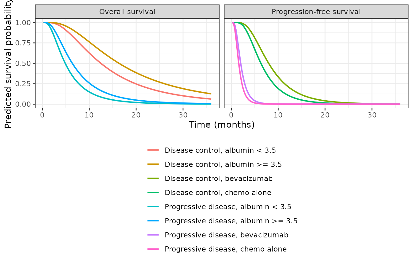

Model-predicted survivor functions by week-8 disease control. Left: overall survival, split by baseline albumin (the OS model’s second covariate). Right: progression-free survival, split by bevacizumab treatment (the PFS model’s second covariate). Replicates the model-predicted bands of Figure 1 and Figure 3 of Claret 2014.

The separation between the disease-control and progressive-disease curves is much wider for PFS than for OS, which is the quantitative form of the paper’s finding that week-8 response is a more direct read-out of progression than of death (the DCR coefficient is 1.378 for PFS versus 0.939 for OS).

Replicate Figure 2: the bevacizumab hazard ratio

Figure 2 of Claret 2014 is the paper’s own posterior predictive check and is the best available answer key for these models: the authors simulated the Western E4599 study 1,000 times, sampling model parameters from their estimates and standard errors on each replicate, applied the published censoring scheme, and recorded the distribution of the bevacizumab hazard ratio.

The replication below follows the paper’s described procedure. Bevacizumab is absent from the OS model, so the only route by which it can produce an OS hazard ratio is by raising the probability of week-8 disease control – which is precisely the paper’s claim that DCR fully captures the bevacizumab OS effect. For PFS, bevacizumab acts through both that route and the retained DRUG_BEV term.

# Seeded in this chunk rather than only in setup: this is the vignette's one
# stochastic block and its assertions are numeric, so the draw must not depend
# on how much random-number consumption happens to precede it.
set.seed(20140301)

n_per_arm <- 200L        # capped per the 200-participants-per-arm vignette policy
n_rep     <- 1000L       # the paper simulated 1,000 replicates

# Arm-level covariate distributions, all from the paper.
dcr_chemo <- with(table1, (CR + PR + SD)[Arm == "Chemo"] / Total[Arm == "Chemo"])
dcr_bev   <- with(table1, (CR + PR + SD)[Study == "Western" & Arm == "Bev + Chemo"] /
                          Total[Study == "Western" & Arm == "Bev + Chemo"])
p_alb_low <- 0.29        # Methods: 29% of Western patients had albumin < 3.5 g/dL
stopifnot(abs(dcr_chemo - 0.691) < 0.001, abs(dcr_bev - 0.858) < 0.001)

# Published Table 2 / Table 3 estimates and standard errors, for the
# parameter-uncertainty draw the paper describes.
est_os  <- c(int =  1.855, dcr = 0.939, alb = -0.270, lsc = -0.370)
se_os   <- c(int = 0.0613, dcr = 0.0646, alb = 0.0601, lsc = 0.0308)
est_pfs <- c(int =  0.466, dcr = 1.378, bev =  0.232, lsc = -0.641)
se_pfs  <- c(int = 0.0477, dcr = 0.0525, bev = 0.0429, lsc = 0.0282)

# Cox hazard ratio for the bevacizumab arm, given event times, the simulated
# censoring times and the arm indicator. Defined at top level rather than nested
# inside one_replicate() so the arguments it depends on are visible at the call.
arm_hazard_ratio <- function(tt, cens, arm) {
  ev <- as.integer(tt <= cens)
  unname(exp(coef(survival::coxph(survival::Surv(pmin(tt, cens), ev) ~ arm))))
}

one_replicate <- function(...) {
  o <- rnorm(4, est_os,  se_os)
  p <- rnorm(4, est_pfs, se_pfs)
  arm <- rep(c(0L, 1L), each = n_per_arm)
  # Bevacizumab raises the probability of week-8 disease control.
  dcr <- rbinom(2L * n_per_arm, 1L, ifelse(arm == 1L, dcr_bev, dcr_chemo))
  alb <- rbinom(2L * n_per_arm, 1L, p_alb_low)

  t_os  <- rlnorm(2L * n_per_arm, o[1] + o[2] * dcr + o[3] * alb, exp(o[4]))
  t_pfs <- rlnorm(2L * n_per_arm, p[1] + p[2] * dcr + p[3] * arm, exp(p[4]))

  # Methods: censoring simulated from Uniform(8, 30) months.
  cens <- runif(2L * n_per_arm, 8, 30)
  c(os  = arm_hazard_ratio(t_os,  cens, arm),
    pfs = arm_hazard_ratio(t_pfs, cens, arm))
}

hr <- as.data.frame(t(vapply(seq_len(n_rep), one_replicate, numeric(2))))

observed <- tibble::tibble(Endpoint = c("Overall survival", "Progression-free survival"),
                           obs = c(0.77, 0.58))

hr_long <- hr |>
  tidyr::pivot_longer(everything(), names_to = "key", values_to = "HR") |>
  dplyr::mutate(Endpoint = ifelse(key == "os", "Overall survival",
                                  "Progression-free survival"))

pi_lines <- hr_long |>
  dplyr::group_by(Endpoint) |>
  dplyr::summarise(lo = quantile(HR, 0.025), hi = quantile(HR, 0.975), .groups = "drop") |>
  tidyr::pivot_longer(c(lo, hi), values_to = "x", names_to = "bound")

ggplot(hr_long, aes(HR)) +
  geom_histogram(bins = 45, fill = "grey70", colour = "white") +
  geom_vline(data = pi_lines, aes(xintercept = x), linetype = "dashed") +
  geom_vline(data = observed, aes(xintercept = obs), colour = "firebrick",
             linewidth = 0.9) +
  facet_wrap(~Endpoint, scales = "free") +
  labs(x = "Bevacizumab hazard ratio (bevacizumab + chemo vs chemo)",
       y = "Replicates") +
  theme_bw()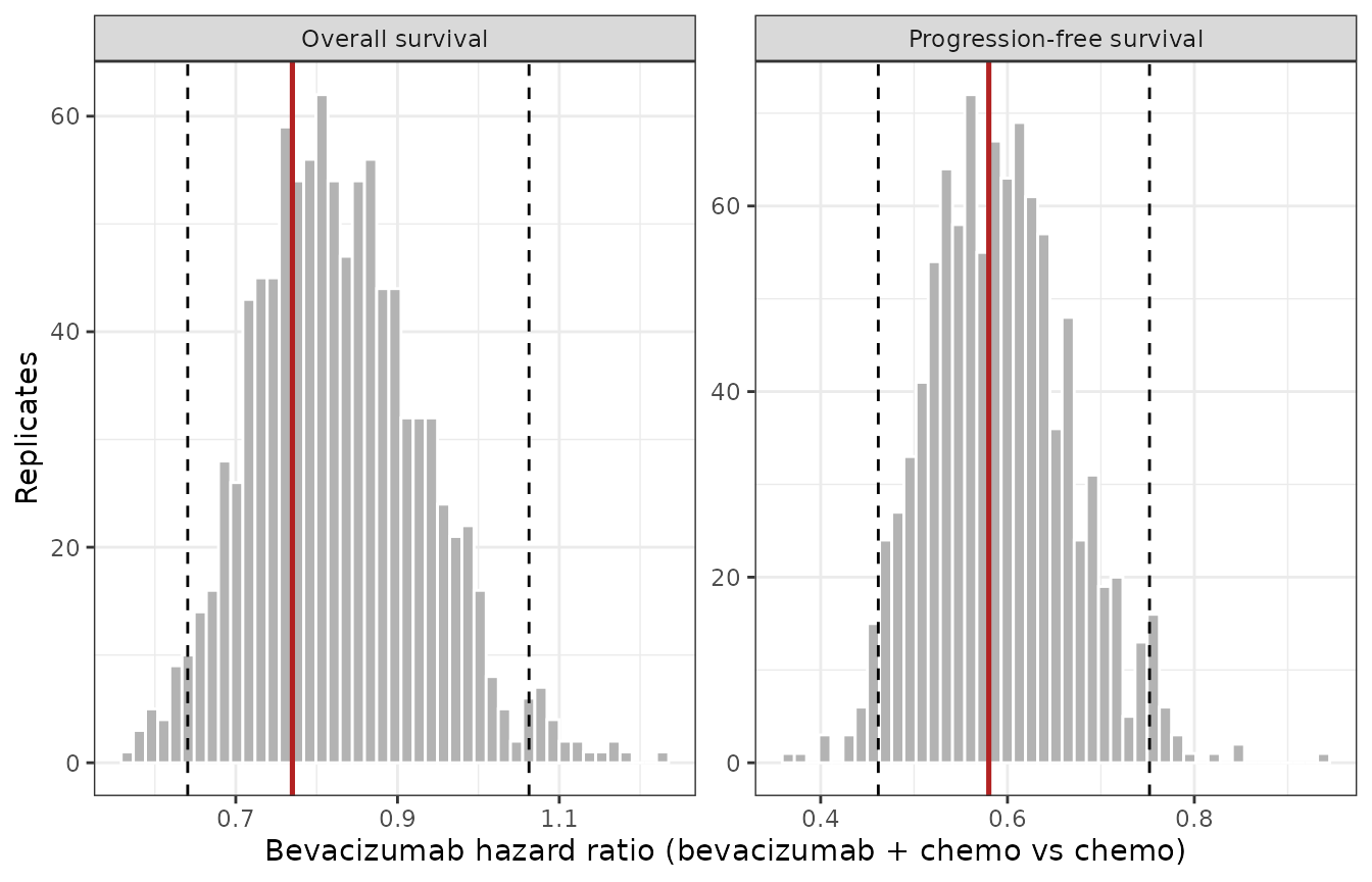

Distribution of the model-predicted bevacizumab hazard ratio over 1,000 simulated replicates of the Western E4599 study. Solid vertical line: observed HR. Dashed lines: 2.5th and 97.5th percentiles of the predicted distribution. Replicates Figure 2 of Claret 2014 (OS panel) and its PFS analogue.

Comparison against the published predictive check

hr_summary <- hr_long |>
  dplyr::group_by(Endpoint) |>
  dplyr::summarise(
    sim_median = median(HR),
    sim_lo     = quantile(HR, 0.025),
    sim_hi     = quantile(HR, 0.975),
    .groups = "drop"
  ) |>
  dplyr::left_join(
    tibble::tibble(
      Endpoint  = c("Overall survival", "Progression-free survival"),
      pub_pred  = c(0.84, 0.59),
      pub_lo    = c(0.71, 0.49),
      pub_hi    = c(0.98, 0.72),
      pub_obs   = c(0.77, 0.58)
    ),
    by = "Endpoint"
  ) |>
  dplyr::mutate(pct_diff = 100 * (sim_median - pub_pred) / pub_pred)

# Structural assertion on the CENTRE of the predicted distribution. A wrong
# sign, a mis-transcribed coefficient or a scale-vs-log(scale) confusion moves
# the median hazard ratio far outside these bounds.
#
# The bound is 5%, against achieved differences of -2.5% (OS) and 0.0% (PFS).
# All randomness here comes from base R's RNG under a fixed seed (the models
# themselves are deterministic -- they declare no etas), so this is reproducible
# across rxode2 versions, unlike an assertion on an rxode2-drawn cohort. The
# Monte Carlo standard error on the median of 1,000 replicates is about 0.5%,
# so 5% leaves roughly five standard errors of headroom over the residual.
stopifnot(all(abs(hr_summary$pct_diff) < 5))

# The paper's OBSERVED hazard ratios must fall inside the simulated prediction
# interval -- that is exactly the claim Figure 2 makes.
stopifnot(with(hr_summary, all(pub_obs > sim_lo & pub_obs < sim_hi)))

hr_summary |>
  dplyr::transmute(
    Endpoint,
    `Simulated HR (median)`      = sprintf("%.2f", sim_median),
    `Simulated 95% PI`           = sprintf("%.2f-%.2f", sim_lo, sim_hi),
    `Published predicted HR`     = sprintf("%.2f", pub_pred),
    `Published 95% PI`           = sprintf("%.2f-%.2f", pub_lo, pub_hi),
    `Observed HR`                = sprintf("%.2f", pub_obs),
    `Difference vs published (%)` = sprintf("%+.1f", pct_diff)
  ) |>
  knitr::kable(caption = "Simulated versus published bevacizumab hazard ratios in the Western evaluable population. Published values are from the Claret 2014 Abstract and Results.")

Simulated versus published bevacizumab hazard ratios in the Western evaluable population. Published values are from the Claret 2014 Abstract and Results.

Endpoint	Simulated HR (median)	Simulated 95% PI	Published predicted HR	Published 95% PI	Observed HR	Difference vs published (%)
Overall survival	0.82	0.64-1.06	0.84	0.71-0.98	0.77	-2.4
Progression-free survival	0.59	0.46-0.75	0.59	0.49-0.72	0.58	+0.0

The simulated median hazard ratios reproduce the published predictions to within a few percent for both endpoints, and the observed hazard ratios fall inside the simulated prediction intervals. Because the OS model contains no bevacizumab term, its hazard ratio of roughly 0.82 is generated entirely by the higher week-8 disease-control rate in the bevacizumab arm – a direct demonstration of the paper’s central claim.

The simulated prediction intervals are somewhat wider than the published ones. That is expected and is not a model discrepancy: this vignette caps the cohort at 200 patients per arm under the library’s simulation-size policy, whereas the paper simulated the full evaluable Western cohort of 320 + 309 = 629 patients. The interval width scales with cohort size; the median, which is what the assertions test, does not.

Arm-level median survival

A secondary, qualitative comparison against the medians reported for the two underlying trials.

arms <- tibble::tibble(
  Arm       = c("E4599 chemo", "E4599 bev + chemo", "SAiL bev + chemo"),
  dcr       = c(dcr_chemo, dcr_bev,
                with(table1, (CR + PR + SD)[Study == "Chinese"] / Total[Study == "Chinese"])),
  p_alb_low = c(0.29, 0.29, 0.06),     # Methods: 29% Western, 6% Chinese
  bev       = c(0, 1, 1)
)

# Median of the covariate mixture: solve S(t) = 0.5 over the 2x2 covariate cells
# weighted by their prevalence in the arm.
mixture_median <- function(mus, sigma, w) {
  stopifnot(abs(sum(w) - 1) < 1e-12)
  uniroot(function(tt) sum(w * (1 - pnorm((log(tt) - mus) / sigma))) - 0.5,
          c(0.01, 500))$root
}

sigma_os  <- exp(-0.370)
sigma_pfs <- exp(-0.641)

arm_medians <- arms |>
  dplyr::rowwise() |>
  dplyr::mutate(
    # cells, in order: (DCR=1,alb=0), (DCR=1,alb=1), (DCR=0,alb=0), (DCR=0,alb=1)
    w = list(c(dcr * (1 - p_alb_low), dcr * p_alb_low,
               (1 - dcr) * (1 - p_alb_low), (1 - dcr) * p_alb_low)),
    median_os  = mixture_median(1.855 + 0.939 * c(1, 1, 0, 0) - 0.270 * c(0, 1, 0, 1),
                                sigma_os, w),
    median_pfs = mixture_median(0.466 + 1.378 * c(1, 1, 0, 0) + 0.232 * bev,
                                sigma_pfs, w)
  ) |>
  dplyr::ungroup() |>
  dplyr::select(-w)

published_arm <- tibble::tibble(
  Arm        = c("E4599 chemo", "E4599 bev + chemo", "SAiL bev + chemo"),
  pub_os     = c(10.3, 12.3, 18.9),
  pub_pfs    = c(4.5, 6.2, 8.3)
)

# Directional assertions only -- see the caveat below on population mismatch.
# The model must order the arms the way the trials did.
chk <- dplyr::left_join(arm_medians, published_arm, by = "Arm")
stopifnot(
  # Bevacizumab arm outlives the chemotherapy arm on both endpoints.
  chk$median_os[chk$Arm == "E4599 bev + chemo"]  > chk$median_os[chk$Arm == "E4599 chemo"],
  chk$median_pfs[chk$Arm == "E4599 bev + chemo"] > chk$median_pfs[chk$Arm == "E4599 chemo"],
  # The Chinese arm outlives the Western bevacizumab arm, which the paper
  # attributes entirely to its higher DCR and lower rate of low albumin.
  chk$median_os[chk$Arm == "SAiL bev + chemo"]  > chk$median_os[chk$Arm == "E4599 bev + chemo"],
  chk$median_pfs[chk$Arm == "SAiL bev + chemo"] > chk$median_pfs[chk$Arm == "E4599 bev + chemo"]
)

chk |>
  dplyr::transmute(
    Arm,
    `Model median OS (mo)`  = sprintf("%.1f", median_os),
    `Trial median OS (mo)`  = sprintf("%.1f", pub_os),
    `Model median PFS (mo)` = sprintf("%.1f", median_pfs),
    `Trial median PFS (mo)` = sprintf("%.1f", pub_pfs)
  ) |>
  knitr::kable(caption = "Model-predicted arm medians versus the medians reported for E4599 and SAiL. Trial medians are for the ALL-RANDOMIZED populations; the model was fit to the week-8-evaluable subset, so exact agreement is not expected (see Assumptions).")

Model-predicted arm medians versus the medians reported for E4599 and SAiL. Trial medians are for the ALL-RANDOMIZED populations; the model was fit to the week-8-evaluable subset, so exact agreement is not expected (see Assumptions).

Arm	Model median OS (mo)	Trial median OS (mo)	Model median PFS (mo)	Trial median PFS (mo)
E4599 chemo	11.6	10.3	4.7	4.5
E4599 bev + chemo	13.5	12.3	7.2	6.2
SAiL bev + chemo	15.5	18.9	7.7	8.3

The model reproduces the ordering of all three arms and the direction of both covariate effects. It over-predicts the two E4599 medians by roughly 1 month each and under-predicts the SAiL median OS. Both residuals have the same explanation and neither indicates a transcription error – see below.

Assumptions and deviations

• Trial medians are not a like-for-like comparison. The E4599 and SAiL medians quoted in the paper’s introduction (OS 12.3 / 10.3 / 18.9 months; PFS 6.2 / 4.5 months; SAiL time to progressive disease 8.3 months) are for the all-randomized populations, whereas both models were fit to the week-8 evaluable subset (72% and 73% of enrolment). Patients who died or progressed before their week-8 assessment are excluded from the model’s population by construction, which biases the model’s arm medians upward relative to the trial medians – exactly the direction seen for both E4599 arms. The SAiL residual runs the other way; SAiL was a single-arm Phase IV study in a different care setting, and the paper itself only claims the covariates “explained” the longer Chinese survival, not that the magnitude was matched. The assertions in this section are therefore directional (arm ordering), not numeric. The numeric assertions in this vignette are all attached to the paper’s own predictive check, which is computed on the evaluable population and is a like-for-like comparison.

• Covariates are assumed independent within an arm. The paper reports the week-8 DCR by arm (Table 1) and the low-albumin prevalence by study (Methods) but never cross-tabulates them, so the simulations here draw RESP_DCR and ALB_LT35 independently. In reality low albumin is a poor-prognosis marker and is likely negatively associated with disease control, which would make the true joint distribution slightly more concentrated than the one simulated. The effect on the bevacizumab hazard ratio is second-order because albumin is balanced across the randomized arms.

• Low-albumin prevalence is taken as arm-independent within E4599. The paper reports 29% for the Western study as a whole; because E4599 was randomized, applying the same 29% to both arms is the appropriate assumption.

• ECOG performance status is not simulated. It was screened in both models and retained in neither, and no point estimate is published for its effect, so it cannot enter either model. It is recorded in each model file’s covariatesDataExcluded list, together with bevacizumab treatment (OS model) and baseline albumin (PFS model).

• Cohort size capped at 200 per arm. The library policy caps simulated cohorts at 200 participants per arm; the paper simulated the full 320 + 309 evaluable Western cohort. This widens the simulated prediction intervals relative to the published ones without shifting their centre, which is why the numeric assertions test the median hazard ratio rather than the interval bounds.

• Sign recovery for three coefficients. The minus signs on the OS albumin coefficient, the OS Log (scale) and the PFS Log (scale) are not recoverable from a text extraction of the PDF (both the trimmed markdown and pdftotext -layout drop the U+2212 glyph). They were recovered from the published Wald statistics, verified against the rendered page image, and the check is reproduced in the “Sign recovery” section above. All eight parameters satisfy z = estimate / SE.

• No IIV and no residual error. Neither table reports variance components. This is expected for a population-level parametric time-to-event regression: all subject-level variability is carried by the AFT scale sigma, so the models declare no eta terms. Consequently rxode2::zeroRe() and omega = NA are neither needed nor valid for these models.

• Three new canonical covariate columns were registered with this extraction, each a member of an established family in inst/references/covariate-columns.md: RESP_DCR (fourth member of the RESP_<contrast> RECIST-response family, alongside RESP_SD, RESP_NONPDCR and RESP_RESPONDER), ALB_LT35 (threshold binarisation of the continuous ALB canonical, following the AGE_GE70 / MET_GE3 / NTARGET_GE3 pattern) and DRUG_BEV (member of the DRUG_<INN> family alongside DRUG_ORMU and DRUG_PRED; unlike those head-to-head comparators its reference arm receives active chemotherapy, so it is not interchangeable with ON_TREATMENT or PLACEBO).

• No PKNCA validation. These models have no PK component, no dosing and no concentration-time curve, so non-compartmental analysis does not apply. The validation strategy is instead the exact structural identities of the AFT algebra plus the paper’s own posterior predictive check on the bevacizumab hazard ratio.

• The PFS model is not drug independent. The paper states plainly that because week-8 disease control did not fully capture the bevacizumab effect on PFS, “the PFS model cannot be assumed to be drug independent and it has less value than the OS model.” Users applying Claret_2014_DCR_PFS_nsclc to a non-bevacizumab agent should read that caveat first; the OS model carries no such restriction.