Overall-survival MBMA in platinum-ineligible NSCLC (Chen 2026)
Source:vignettes/articles/Chen_2026_nsclc_os_mbma.Rmd
Chen_2026_nsclc_os_mbma.Rmd- Citation: Chen J, Wada R, Zhang N, Graupner V, Morris S, Hu Y, Zhang W, Kassir N, Wu B, Chan P. Model-Based Meta-Analysis of Overall Survival in Vulnerable Platinum-Ineligible NSCLC Populations. CPT Pharmacometrics Syst Pharmacol. 2026;15:e70197. doi:10.1002/psp4.70197. Parameter values are Table S8 (‘Final Model Parameters (mod010)’) of the Supporting Information; the model structure is the NONMEM $PRED block distributed as Supporting Information file psp470197-sup-0002-Supinfo2.ctl.
- Article: CPT Pharmacometrics Syst Pharmacol. 2026;15:e70197
Model and source
Chen 2026 asks a question that model-based meta-analysis (MBMA) is rarely used for: not whether the investigational arm of a registrational trial works, but whether its control arm was a fair comparator. The phase III IPSOS trial (NCT03191786) compared atezolizumab monotherapy against single-agent chemotherapy in treatment-naive advanced non-small cell lung cancer (NSCLC) patients unsuitable for platinum-doublet chemotherapy, but its protocol restricted the control arm to gemcitabine or vinorelbine. Both the NCCN and the ESMO guidelines list a broader set of single agents for this population, so the authors assembled a literature database of historical single-agent trials and asked whether the IPSOS control arm was non-inferior to that broader set.
The model is a mixed-effects non-parametric conditional-probability survival model, fitted in NONMEM 7.5.1 by the Laplacian method to digitised Kaplan-Meier curves. Its two moving parts are:
- A reference survival curve with no assumed shape. The logit of the reference survival probability is an estimated monotone random walk over 30 knots (months 1-24, then 27, 30, 33, 36, 42 and 48). The reference is a historical single-agent-chemotherapy control arm composed entirely of ECOG performance status 0 patients.
- A proportional rescaling of that curve per study
arm,
S_arm(t) = S_ref(t)^exp(log(HR)), wherelog(HR)is a linear combination of covariates plus a between-trial random effect. BecauseS = exp(-H), raising the survival function to the powerexp(log(HR))multiplies the cumulative hazard by the hazard ratio, so this is an ordinary proportional-hazards model written on the survival scale.
This file encodes the paper’s final model, Model 010, whose complete parameter set is Table S8 of the Supporting Information.
mod
#>  ── rxode2-based Pred model ─────────────────────────────────────────────────────
#>  ── Initalization: ──
#> Fixed Effects ($theta):
#>  lgtsurv_01 dlgtsurv_02 dlgtsurv_03 dlgtsurv_04 dlgtsurv_05 dlgtsurv_06
#>       2.802       0.831       0.520       0.401       0.301       0.258
#> dlgtsurv_07 dlgtsurv_08 dlgtsurv_09 dlgtsurv_10 dlgtsurv_11 dlgtsurv_12
#>       0.189       0.196       0.159       0.152       0.143       0.114
#> dlgtsurv_13 dlgtsurv_14 dlgtsurv_15 dlgtsurv_16 dlgtsurv_17 dlgtsurv_18
#>       0.099       0.168       0.102       0.098       0.094       0.083
#> dlgtsurv_19 dlgtsurv_20 dlgtsurv_21 dlgtsurv_22 dlgtsurv_23 dlgtsurv_24
#>       0.115       0.187       0.051       0.093       0.105       0.135
#> dlgtsurv_27 dlgtsurv_30 dlgtsurv_33 dlgtsurv_36 dlgtsurv_42 dlgtsurv_48
#>       0.137       0.225       0.260       0.442       0.517       0.000
#>     e_ecog1    e_ecog23  e_ipsosctl
#>       0.004       0.769      -0.633
#>
#> Omega ($omega):
#>           eta_study
#> eta_study  0.066049
#> attr(,"lotriFix")
#>           eta_study
#> eta_study      TRUE
#>  ── Model (Normalized Syntax): ──
#> function() {
#>     covariateData <- list(PS_ECOG_1_PCT = list(description = "Study-arm-level percentage (0-100) of the enrolled cohort with an ECOG performance status of 1 at baseline.",
#>         units = "%", type = "continuous", reference_category = "0% (no ECOG-1 patients). The model's reference arm is PS_ECOG_1_PCT = PS_ECOG_2_PCT = PS_ECOG_3_PCT = 0, i.e. an all-ECOG-0 arm.",
#>         source_name = "PS1 (Chen 2026 NONMEM dataset psp470197-sup-0001-Supinfo1.csv $INPUT); 'PS.1' (Chen 2026 Tables S5 and S6); 'ECOG PS 1 (%)' (Chen 2026 Table 2)",
#>         notes = "MBMA study-arm-level covariate, scaled in PERCENT (0-100), not a fraction -- the model divides by 100 internally, matching ECOGEFF = COVECOG1*PS1/100 in the source control stream. Enters log(HR) with coefficient e_ecog1 = 0.004, i.e. hazard ratio exp(0.004) = 1.004 for an arm that is 100% ECOG 1 relative to an all-ECOG-0 arm (Chen 2026 Table 3, Model 010, ECOG1HR column). The estimate is essentially null and very imprecisely determined (RSE 11922%, 95% CI 0.412-2.443), which the paper reports as-is; it is retained because Model 010 estimates the ECOG effects from the MBMA data rather than fixing them. Across the 41 analysis arms the median is 42.9% (range 0.0-69.6; Chen 2026 Table 2). PS_ECOG_0_PCT, PS_ECOG_1_PCT, PS_ECOG_2_PCT and PS_ECOG_3_PCT sum to 100 within an arm, so supplying all four is redundant; the model consumes only PS 1, 2 and 3 and treats ECOG 0 as the reference level. Distinct from the per-subject binaries ECOG_GE1 / ECOG_GE2, which are individual-level indicators. Family member of PS_ECOG_0_PCT (founding example Franzese 2026). Chen 2026 Methods 2.2 notes that 30 of the ECOG PS percentages in the database were IMPUTED -- first by mapping Karnofsky Performance Scores where available, otherwise by splitting composite ECOG categories with a logistic regression calibrated on studies with similar entry criteria."),
#>         PS_ECOG_2_PCT = list(description = "Study-arm-level percentage (0-100) of the enrolled cohort with an ECOG performance status of 2 at baseline.",
#>             units = "%", type = "continuous", reference_category = "0% (no ECOG-2 patients); ECOG 0 is the model's reference performance-status level.",
#>             source_name = "PS2 (Chen 2026 NONMEM dataset psp470197-sup-0001-Supinfo1.csv $INPUT); 'PS.2' (Chen 2026 Tables S5 and S6)",
#>             notes = "MBMA study-arm-level covariate, scaled in PERCENT (0-100). PS_ECOG_2_PCT and PS_ECOG_3_PCT SHARE a single coefficient in this model: the source control stream computes ECOGEFF using COVECOG2*(PS2+PS3)/100, so ECOG 2 and ECOG 3 are pooled into one composite effect (e_ecog23 = 0.769, hazard ratio 2.158; Chen 2026 Table 3 Model 010 ECOG2,3HR column). They are kept as two separate columns rather than a single pooled PS_ECOG_23_PCT because the source dataset carries them separately and because Chen 2026 Table 2 reports them pooled while Tables S5/S6 report them apart. Pooled across ECOG 2 and 3, the median across the 41 analysis arms is 28.8% (range 0.0-100.0; Chen 2026 Table 2). The pooled ECOG-2/3 percentage is the single most load-bearing covariate in the paper: the IPSOS control arm is 87.4% ECOG 2 or 3 (76.8% + 10.6%), against a database median of 28.8%, which is why adjusting for performance status moves the IPSOS-versus-historical hazard ratio from 0.812 (Model 007a, unadjusted) to 0.531 (Model 010, adjusted). See PS_ECOG_1_PCT for the imputation caveat, which applies equally here."),
#>         PS_ECOG_3_PCT = list(description = "Study-arm-level percentage (0-100) of the enrolled cohort with an ECOG performance status of 3 at baseline.",
#>             units = "%", type = "continuous", reference_category = "0% (no ECOG-3 patients); ECOG 0 is the model's reference performance-status level.",
#>             source_name = "PS3 (Chen 2026 NONMEM dataset psp470197-sup-0001-Supinfo1.csv $INPUT); 'PS.3' (Chen 2026 Tables S5 and S6)",
#>             notes = "MBMA study-arm-level covariate, scaled in PERCENT (0-100). Shares the coefficient e_ecog23 with PS_ECOG_2_PCT -- see the PS_ECOG_2_PCT notes for why the two are pooled and why they are nevertheless carried as separate columns. ECOG 3 is rare in this database: it is non-zero in only four of the 41 arms (Chen 2026 Table S6), the largest being the IPSOS trial arms (10.6% in the control arm)."),
#>         TRT_IPSOS_CONTROL = list(description = "Indicator that the study arm is the control arm of the phase III IPSOS trial (NCT03191786, reported as Lee 2023), in which investigators chose single-agent gemcitabine or vinorelbine.",
#>             units = "(binary)", type = "binary", reference_category = "0 (a historical single-agent-chemotherapy control arm from the published literature -- the model's reference treatment)",
#>             source_name = "ID == 15 with the atezolizumab arm excluded (Chen 2026 NONMEM dataset psp470197-sup-0001-Supinfo1.csv; the source control stream selects the trial arm with IF (ID.EQ.15))",
#>             notes = "MBMA trial-arm indicator, NOT a patient characteristic. 1 = the IPSOS control arm (Lee 2023, ID 15, ARM 2, n = 151, drug code 3 = 'gemcitabine or vinorelbine'); 0 = any of the 39 historical control arms. Enters log(HR) with coefficient e_ipsosctl = -0.633, i.e. hazard ratio exp(-0.633) = 0.531 (95% CI 0.424-0.664), reproducing the IPSOSHR column of Chen 2026 Table 3 for Model 010. Model 010 is fitted with the IPSOS ATEZOLIZUMAB arm EXCLUDED from the dataset (Chen 2026 Table 5, Data column), so within this model the IPSOS trial identifier and the IPSOS control arm are the same thing. Do NOT set this flag on an atezolizumab arm: the atezolizumab effect belongs to Model 041, whose reference survival curve Chen 2026 does not publish (see vignette Errata). The paper's headline hazard ratios of 0.543 (IPSOS control) and 0.418 (IPSOS atezolizumab) versus historical trials come from Model 041, not Model 010; Model 010's 0.531 is the corresponding quantity in the final model. Family member of the TRT_<arm> treatment-arm-indicator canonicals (TRT_EPHEDRINE, TRT_PBT, TRT_PCSK9I, ...)."))
#>     covariatesDataExcluded <- list(AGE = list(description = "Median age of the patients in the study arm.",
#>         units = "years", type = "continuous", notes = "Screened as a candidate covariate on log(HR) (tested as an age category) and not retained. Median across arms 74.0 years, range 61.0-79.0 (Chen 2026 Table 2). Source column 'Age' (Table S1)."),
#>         SEXM_PCT = list(description = "Percentage (0-100) of the study arm who are male.",
#>             units = "%", type = "continuous", notes = "Screened and not retained; Model 012 gave a covariate HR of 1.070 (95% CI 0.387-2.954) with dOBJ = +0.0 versus Model 008 (Chen 2026 Table S7). Median across arms 74.7%, range 38.9-94.2 (Table 2). Source column 'MaleP' (Table S1). Recorded as a male percentage because that is the direction the source reports; the individual-level canonical SEXF is coded 1 = female."),
#>         DIS_STAGE4_PCT = list(description = "Percentage (0-100) of the study arm with Stage IV (metastatic) disease.",
#>             units = "%", type = "continuous", notes = "Screened and not retained; Model 011 gave a covariate HR of 0.624 (95% CI 0.210-1.852) (Chen 2026 Table S7). Median across arms 73.1%, range 41.3-88.9 (Table 2). Source column 'Stage4' (Tables S5 and S6)."),
#>         TUMTP_SQUAM_PCT = list(description = "Percentage (0-100) of the study arm with squamous-cell histology.",
#>             units = "%", type = "continuous", notes = "Screened and not retained; Model 013 gave a covariate HR of 1.125 (95% CI 0.454-2.788) (Chen 2026 Table S7). Median across arms 39.3%, range 0.0-54.4 (Table 2). Three squamous percentages were imputed (Chen 2026 Section 3.1.2). Source column 'SquamousP' (Table S1)."),
#>         TUMTP_ADENO_PCT = list(description = "Percentage (0-100) of the study arm with adenocarcinoma histology.",
#>             units = "%", type = "continuous", notes = "Screened and not retained; Model 014 gave a covariate HR of 0.625 (95% CI 0.250-1.560) (Chen 2026 Table S7). Median across arms 39.3%, range 14.0-87.0 (Table 2). Five adenocarcinoma percentages were imputed (Chen 2026 Section 3.1.2). Source column 'AdenoP' (Table S1)."),
#>         RACE_ASIAN_PCT = list(description = "Percentage (0-100) of the study arm enrolled in Asia.",
#>             units = "%", type = "continuous", notes = "Screened and not retained; Model 015 gave a covariate HR of 0.817 (95% CI 0.658-1.015) (Chen 2026 Table S7). Bimodal across arms -- median 0.0% with range 0.0-100.0 (Table 2), because trials were either wholly Asian or wholly non-Asian. Tested because Asian patients may survive longer on immune-checkpoint-inhibitor therapy (Chen 2026 Section 2.2). Source column 'Asia' (Tables S5 and S6)."),
#>         YEAR_PUBLICATION = list(description = "Calendar year in which the trial was published.",
#>             units = "year", type = "continuous", notes = "Screened as a time-trend covariate and not retained: Model 049 reduced the objective function by only 3.3 points against the 6.635 required (Chen 2026 Table 5). The coefficient was negative (more recent publication associated with lower hazard), consistent with medical practice improving over time, and including it widened the IPSOS hazard ratio to 0.780 (95% CI 0.479-1.269), a CI that includes 1. Source column 'YEAR' (NONMEM dataset)."))
#>     description <- "MBMA. Mixed-effects non-parametric conditional-probability model-based meta-analysis (MBMA) of OVERALL SURVIVAL in treatment-naive, locally advanced or metastatic non-small cell lung cancer (NSCLC) patients who are ineligible for platinum-doublet chemotherapy (ECOG performance status >= 2, or age >= 70 years, or investigator-determined platinum ineligibility). Chen 2026 digitised Kaplan-Meier overall-survival curves from 26 published trials (41 arms, 3637 participants) of single-agent docetaxel, gemcitabine, paclitaxel, pemetrexed or vinorelbine, and compared them against the control arm of the phase III IPSOS trial (NCT03191786, Lee 2023), in which investigators chose gemcitabine or vinorelbine. This file encodes the paper's FINAL model, Model 010, whose complete parameter set is Chen 2026 Table S8. The survival model is semi-parametric proportional hazards with a NON-PARAMETRIC reference survival curve: the logit of the reference survival probability follows an estimated random walk over 30 knots (months 1-24, then 27, 30, 33, 36, 42 and 48), and every study arm is a proportional rescaling of it, S_arm(t) = S_ref(t)^exp(log(HR)). The reference is a historical single-agent-chemotherapy control arm composed entirely of ECOG performance status 0 patients. log(HR) is a linear combination of the arm's ECOG-PS-1 and ECOG-PS-2/3 percentages, an IPSOS-control-arm indicator, and a between-trial random effect (SD 0.257). ECOG performance status was the ONLY covariate that reached statistical significance; age, sex, disease stage, squamous and adenocarcinoma histology, Asian region and publication year were all screened and rejected (see covariatesDataExcluded). All parameter values are wrapped in fixed() because the model is a downstream user of the published fit, not a re-estimation of it. Simulation scope: per-ARM overall-survival curves over the 1-48 month window the digitised data support. The random effect is BETWEEN-TRIAL, not between-subject, so this model predicts trial-arm mean survival curves and is NOT suitable for individual-subject time-to-event simulation. No residual error is estimated: Chen 2026 fits a user-supplied binomial -2LL on the number of deaths per interval rather than a residual-error model, so there is no $SIGMA to encode and no observation endpoint is declared. Companion paper in the same issue: Franzese_2026_pdl1_nsclc_mbma."
#>     paper_specific_etas <- "eta_study"
#>     population <- list(species = "human", n_subjects = 3637L,
#>         n_studies = 26L, n_arms = 41L, age_range = "Arm-level median age 74.0 years, range across arms 61.0-79.0 (Chen 2026 Table 2). Individual ages are not available: this is a summary-level meta-analysis.",
#>         weight_range = "Not collected. Body weight is not a covariate in any Chen 2026 model and is not reported in the analysis database.",
#>         sex_female_pct = 25.3, disease_state = "Treatment-naive, locally advanced or metastatic non-small cell lung cancer in patients unsuitable for platinum-doublet chemotherapy. Eligibility for the literature database required ECOG performance status >= 2, or age >= 70 years, or platinum ineligibility as defined by the respective published study. Arm-level medians (range) across the 41 arms: ECOG PS 0 14.7% (0.0-57.4), ECOG PS 1 42.9% (0.0-69.6), ECOG PS 2 or 3 28.8% (0.0-100.0), Stage IV disease 73.1% (41.3-88.9), squamous histology 39.3% (0.0-54.4), adenocarcinoma histology 39.3% (14.0-87.0) (Chen 2026 Table 2).",
#>         dose_range = "Not modelled. Chen 2026 carries treatment identity, not dose: no dose, schedule or exposure metric enters any model.",
#>         regions = "Multinational. Arm-level percentage enrolled in Asia has median 0.0% and range 0.0-100.0 (Chen 2026 Table 2) -- the constituent trials were each wholly Asian or wholly non-Asian.",
#>         treatments = "Single-agent chemotherapy by drug (Chen 2026 Table 1, studies / arms / n): docetaxel 7 / 11 / 711; gemcitabine 10 / 12 / 969; gemcitabine or vinorelbine 2 / 2 / 341; paclitaxel 3 / 3 / 311; pemetrexed 2 / 2 / 90; vinorelbine 9 / 10 / 913; atezolizumab 1 / 1 / 302. Studies sum to more than 26 because some trials contributed more than one drug.",
#>         notes = "SUMMARY-LEVEL meta-analysis. Each 'subject' in nlmixr2 corresponds to one study-strata-arm, carrying that arm's mean covariate values and its digitised Kaplan-Meier overall-survival curve; the random effect eta_study is BETWEEN-TRIAL, not between-subject. sex_female_pct is DERIVED as 100 minus the arm-level MEDIAN male percentage of 74.7% (Chen 2026 Table 2); it is a median across arms rather than a participant-weighted pooled percentage, which the paper does not report. Data were obtained by digitising published Kaplan-Meier curves at monthly intervals with Engauge Digitizer 12.1 (Chen 2026 Section 2.2); censoring tick marks could not be recovered, so the analysis is of conditional death probabilities per interval rather than of individual event times. Model 010 as encoded here is fitted with the IPSOS ATEZOLIZUMAB arm (n = 302) excluded, leaving 3335 participants across 40 arms (Chen 2026 Table 5, Data column). Curve tails were trimmed before fitting wherever fewer than 10 patients remained at risk or the survival probability fell below 0.1 (the FLAG = 1 and FLAG = 2 exclusions in the distributed dataset), which is why the knot grid stops at 48 months and why the last interval is unidentifiable and fixed to zero. The literature search covered PubMed to 18 September 2023 and returned 275 references, of which 28 (26 unique studies) were retained; a funnel plot showed no material publication bias (Chen 2026 Figure S3).")
#>     reference <- "Chen J, Wada R, Zhang N, Graupner V, Morris S, Hu Y, Zhang W, Kassir N, Wu B, Chan P. Model-Based Meta-Analysis of Overall Survival in Vulnerable Platinum-Ineligible NSCLC Populations. CPT Pharmacometrics Syst Pharmacol. 2026;15:e70197. doi:10.1002/psp4.70197. Parameter values are Table S8 ('Final Model Parameters (mod010)') of the Supporting Information; the model structure is the NONMEM $PRED block distributed as Supporting Information file psp470197-sup-0002-Supinfo2.ctl."
#>     units <- list(time = "month", dosing = "probability", concentration = "probability/probability")
#>     vignette <- "Chen_2026_nsclc_os_mbma"
#>     ini({
#>         lgtsurv_01 <- fix(2.802)
#>         label("Logit of reference overall-survival probability at 1 month (logit scale)")
#>         dlgtsurv_02 <- fix(0.831)
#>         label("Decrement in logit reference survival from month 1 to month 2 (logit scale)")
#>         dlgtsurv_03 <- fix(0.52)
#>         label("Decrement in logit reference survival from month 2 to month 3 (logit scale)")
#>         dlgtsurv_04 <- fix(0.401)
#>         label("Decrement in logit reference survival from month 3 to month 4 (logit scale)")
#>         dlgtsurv_05 <- fix(0.301)
#>         label("Decrement in logit reference survival from month 4 to month 5 (logit scale)")
#>         dlgtsurv_06 <- fix(0.258)
#>         label("Decrement in logit reference survival from month 5 to month 6 (logit scale)")
#>         dlgtsurv_07 <- fix(0.189)
#>         label("Decrement in logit reference survival from month 6 to month 7 (logit scale)")
#>         dlgtsurv_08 <- fix(0.196)
#>         label("Decrement in logit reference survival from month 7 to month 8 (logit scale)")
#>         dlgtsurv_09 <- fix(0.159)
#>         label("Decrement in logit reference survival from month 8 to month 9 (logit scale)")
#>         dlgtsurv_10 <- fix(0.152)
#>         label("Decrement in logit reference survival from month 9 to month 10 (logit scale)")
#>         dlgtsurv_11 <- fix(0.143)
#>         label("Decrement in logit reference survival from month 10 to month 11 (logit scale)")
#>         dlgtsurv_12 <- fix(0.114)
#>         label("Decrement in logit reference survival from month 11 to month 12 (logit scale)")
#>         dlgtsurv_13 <- fix(0.099)
#>         label("Decrement in logit reference survival from month 12 to month 13 (logit scale)")
#>         dlgtsurv_14 <- fix(0.168)
#>         label("Decrement in logit reference survival from month 13 to month 14 (logit scale)")
#>         dlgtsurv_15 <- fix(0.102)
#>         label("Decrement in logit reference survival from month 14 to month 15 (logit scale)")
#>         dlgtsurv_16 <- fix(0.098)
#>         label("Decrement in logit reference survival from month 15 to month 16 (logit scale)")
#>         dlgtsurv_17 <- fix(0.094)
#>         label("Decrement in logit reference survival from month 16 to month 17 (logit scale)")
#>         dlgtsurv_18 <- fix(0.083)
#>         label("Decrement in logit reference survival from month 17 to month 18 (logit scale)")
#>         dlgtsurv_19 <- fix(0.115)
#>         label("Decrement in logit reference survival from month 18 to month 19 (logit scale)")
#>         dlgtsurv_20 <- fix(0.187)
#>         label("Decrement in logit reference survival from month 19 to month 20 (logit scale)")
#>         dlgtsurv_21 <- fix(0.051)
#>         label("Decrement in logit reference survival from month 20 to month 21 (logit scale)")
#>         dlgtsurv_22 <- fix(0.093)
#>         label("Decrement in logit reference survival from month 21 to month 22 (logit scale)")
#>         dlgtsurv_23 <- fix(0.105)
#>         label("Decrement in logit reference survival from month 22 to month 23 (logit scale)")
#>         dlgtsurv_24 <- fix(0.135)
#>         label("Decrement in logit reference survival from month 23 to month 24 (logit scale)")
#>         dlgtsurv_27 <- fix(0.137)
#>         label("Decrement in logit reference survival from month 24 to month 27 (logit scale)")
#>         dlgtsurv_30 <- fix(0.225)
#>         label("Decrement in logit reference survival from month 27 to month 30 (logit scale)")
#>         dlgtsurv_33 <- fix(0.26)
#>         label("Decrement in logit reference survival from month 30 to month 33 (logit scale)")
#>         dlgtsurv_36 <- fix(0.442)
#>         label("Decrement in logit reference survival from month 33 to month 36 (logit scale)")
#>         dlgtsurv_42 <- fix(0.517)
#>         label("Decrement in logit reference survival from month 36 to month 42 (logit scale)")
#>         dlgtsurv_48 <- fix(0)
#>         label("Decrement in logit reference survival from month 42 to month 48 (logit scale); held constant at zero")
#>         e_ecog1 <- fix(0.004)
#>         label("Change in log(HR) for overall survival when an arm is 100% ECOG performance status 1 rather than 100% ECOG 0 (log hazard ratio)")
#>         e_ecog23 <- fix(0.769)
#>         label("Change in log(HR) for overall survival when an arm is 100% ECOG performance status 2 or 3 rather than 100% ECOG 0 (log hazard ratio)")
#>         e_ipsosctl <- fix(-0.633)
#>         label("Change in log(HR) for overall survival in the IPSOS control arm relative to a historical single-agent-chemotherapy control arm (log hazard ratio)")
#>         eta_study ~ fix(0.066049)
#>     })
#>     model({
#>         dlgtsurv_cum <- (t >= 2) * dlgtsurv_02 + (t >= 3) * dlgtsurv_03 +
#>             (t >= 4) * dlgtsurv_04 + (t >= 5) * dlgtsurv_05 +
#>             (t >= 6) * dlgtsurv_06 + (t >= 7) * dlgtsurv_07 +
#>             (t >= 8) * dlgtsurv_08 + (t >= 9) * dlgtsurv_09 +
#>             (t >= 10) * dlgtsurv_10 + (t >= 11) * dlgtsurv_11 +
#>             (t >= 12) * dlgtsurv_12 + (t >= 13) * dlgtsurv_13 +
#>             (t >= 14) * dlgtsurv_14 + (t >= 15) * dlgtsurv_15 +
#>             (t >= 16) * dlgtsurv_16 + (t >= 17) * dlgtsurv_17 +
#>             (t >= 18) * dlgtsurv_18 + (t >= 19) * dlgtsurv_19 +
#>             (t >= 20) * dlgtsurv_20 + (t >= 21) * dlgtsurv_21 +
#>             (t >= 22) * dlgtsurv_22 + (t >= 23) * dlgtsurv_23 +
#>             (t >= 24) * dlgtsurv_24 + (t >= 27) * dlgtsurv_27 +
#>             (t >= 30) * dlgtsurv_30 + (t >= 33) * dlgtsurv_33 +
#>             (t >= 36) * dlgtsurv_36 + (t >= 42) * dlgtsurv_42 +
#>             (t >= 48) * dlgtsurv_48
#>         lgtsurv0 <- lgtsurv_01 - dlgtsurv_cum
#>         surv0 <- (t < 1) * 1 + (t >= 1) * exp(lgtsurv0)/(1 +
#>             exp(lgtsurv0))
#>         lhr <- e_ecog1 * (PS_ECOG_1_PCT/100) + e_ecog23 * ((PS_ECOG_2_PCT +
#>             PS_ECOG_3_PCT)/100) + e_ipsosctl * TRT_IPSOS_CONTROL +
#>             eta_study
#>         hr <- exp(lhr)
#>         surv <- surv0^hr
#>     })
#> }
Population
| Field | Value |
|---|---|
| Species | human |
| Studies | 26 |
| Arms | 41 |
| Participants | 3637 |
| Disease | Treatment-naive locally advanced or metastatic NSCLC, unsuitable for platinum-doublet chemotherapy |
| Age | Arm-level median 74.0 years (range across arms 61.0 to 79.0) |
| Sex | Arm-level median 74.7% male (range 38.9 to 94.2) |
| Region | Multinational; arm-level Asian enrolment median 0%, range 0 to 100 |
| Treatments | Single-agent docetaxel, gemcitabine, paclitaxel, pemetrexed or vinorelbine |
Eligibility for the database required ECOG performance status
>= 2, or age >= 70
years, or platinum ineligibility as defined by the
respective published study. Arm-level performance-status composition is
the covariate that carries the whole analysis: median 14.7% ECOG 0,
42.9% ECOG 1 and 28.8% ECOG 2 or 3 across the 41 arms.
Model 010 is fitted with the IPSOS atezolizumab arm excluded (Chen 2026 Table 5), leaving 3335 participants across 40 arms.
Source trace
Every value in ini() comes from Table S8 (“Final Model
Parameters (mod010)”) of the Supporting Information, except the final
reference-curve decrement, which was fixed to zero and therefore does
not appear there.
| Quantity | Source location |
|---|---|
| logit S_ref(1 month) | Table S8 row 1 (‘logit(Survival at 1-mo)’) = 2.802 |
| 29 logit decrements, months 2-48 | Table S8 rows 2-29 |
| Decrement for months 42 to 48 | Control stream psp470197-sup-0002-Supinfo2.ctl, $THETA row 30: ‘0 FIX ; TIME48’ |
| ECOG PS 1 effect on log(HR) | Table S8 ‘ECOG1 effect’ = 0.004; Table 3 Model 010 ECOG1HR = 1.004 |
| ECOG PS 2 or 3 effect on log(HR) | Table S8 ‘ECOG2,3 effect’ = 0.769; Table 3 Model 010 ECOG2,3HR = 2.158 |
| IPSOS control arm effect on log(HR) | Table S8 ‘IPSOS control arm effect’ = -0.633; Table 3 Model 010 IPSOSHR = 0.531 |
| Between-trial SD on log(HR) | Table S8 ‘Between-trial SD’ = 0.257; $OMEGA is ‘1 FIX’ so this THETA is an SD |
| Random-walk / proportional-hazards structure | Control stream $PRED block; Methods 2.4 and Figure 1 |
| Knot grid (months 1-24, 27, 30, 33, 36, 42, 48) | TIME column of the distributed dataset psp470197-sup-0001-Supinfo1.csv |
| Arm-level ECOG percentages | Tables S5 (raw) and S6 (with imputations); dataset columns PS0-PS3 |
| IPSOS control arm identity | Dataset ID 15 ARM 2 (Lee 2023, gemcitabine or vinorelbine, n = 151) |
Table S8 is internally consistent: its printed RSE column reproduces
as SE / Value * 100 for every row, which is how the
transcription above was checked.
Reference survival curve
The first validation is closed-form and deterministic. The model’s
surv0 output at each knot must equal the inverse logit of
the Table S8 cumulative sum, with no simulation error and no random draw
involved.
knots <- c(1:24, 27, 30, 33, 36, 42, 48)

# Table S8 rows 1-29, transcribed independently of the model file, plus the
# month 42-48 decrement fixed to zero in the control stream.
lgtsurv_01 <- 2.802
decrements <- c(
  0.831, 0.520, 0.401, 0.301, 0.258, 0.189, 0.196, 0.159, 0.152, 0.143,
  0.114, 0.099, 0.168, 0.102, 0.098, 0.094, 0.083, 0.115, 0.187, 0.051,
  0.093, 0.105, 0.135, 0.137, 0.225, 0.260, 0.442, 0.517, 0.000
)
stopifnot(length(decrements) == length(knots) - 1L)

expected_lgt  <- lgtsurv_01 - cumsum(c(0, decrements))
expected_surv <- plogis(expected_lgt)

# Solve the packaged model on an all-ECOG-0 historical control arm, which is
# the reference by construction, at the typical value of the between-trial
# random effect.
ref_arm <- data.frame(
  id = 1L, time = knots, evid = 0L, amt = NA_real_,
  PS_ECOG_1_PCT = 0, PS_ECOG_2_PCT = 0, PS_ECOG_3_PCT = 0,
  TRT_IPSOS_CONTROL = 0
)
ref_sim <- rxode2::rxSolve(
  rxode2::zeroRe(mod), ref_arm, returnType = "data.frame"
)
#> Warning: No sigma parameters in the model
#> ℹ omega/sigma items treated as zero: 'eta_study'

stopifnot(nrow(ref_sim) == length(knots))
max_abs_err <- max(abs(ref_sim$surv0 - expected_surv))
max_abs_err
#> [1] 1.387779e-16

# Deterministic identity: the two sides are the same arithmetic, so this is
# pure floating-point error and a tight bound is correct here. It goes red on
# any mis-transcribed decrement, a knot placed at the wrong month, or a sign
# error in the random walk.
stopifnot(max_abs_err < 1e-10)

# The reference arm must have hazard ratio exactly 1 -- that is what makes it
# the reference.
stopifnot(max(abs(ref_sim$hr - 1)) < 1e-12)
stopifnot(max(abs(ref_sim$surv - ref_sim$surv0)) < 1e-12)| Month | logit S_ref | S_ref (Table S8) | S_ref (model) |
|---|---|---|---|
| 1 | 2.802 | 0.9428 | 0.9428 |
| 2 | 1.971 | 0.8777 | 0.8777 |
| 3 | 1.451 | 0.8102 | 0.8102 |
| 4 | 1.050 | 0.7408 | 0.7408 |
| 5 | 0.749 | 0.6790 | 0.6790 |
| 6 | 0.491 | 0.6203 | 0.6203 |
| 7 | 0.302 | 0.5749 | 0.5749 |
| 8 | 0.106 | 0.5265 | 0.5265 |
| 9 | -0.053 | 0.4868 | 0.4868 |
| 10 | -0.205 | 0.4489 | 0.4489 |
| 11 | -0.348 | 0.4139 | 0.4139 |
| 12 | -0.462 | 0.3865 | 0.3865 |
| 13 | -0.561 | 0.3633 | 0.3633 |
| 14 | -0.729 | 0.3254 | 0.3254 |
| 15 | -0.831 | 0.3034 | 0.3034 |
| 16 | -0.929 | 0.2831 | 0.2831 |
| 17 | -1.023 | 0.2644 | 0.2644 |
| 18 | -1.106 | 0.2486 | 0.2486 |
| 19 | -1.221 | 0.2278 | 0.2278 |
| 20 | -1.408 | 0.1965 | 0.1965 |
| 21 | -1.459 | 0.1886 | 0.1886 |
| 22 | -1.552 | 0.1748 | 0.1748 |
| 23 | -1.657 | 0.1602 | 0.1602 |
| 24 | -1.792 | 0.1428 | 0.1428 |
| 27 | -1.929 | 0.1269 | 0.1269 |
| 30 | -2.154 | 0.1040 | 0.1040 |
| 33 | -2.414 | 0.0821 | 0.0821 |
| 36 | -2.856 | 0.0544 | 0.0544 |
| 42 | -3.373 | 0.0332 | 0.0332 |
| 48 | -3.373 | 0.0332 | 0.0332 |
The reference curve crosses 50% survival between months 8 and 9, giving a median overall survival of roughly 8.7 months for a historical single-agent-chemotherapy arm made up entirely of ECOG 0 patients.
# Interpolate over the strictly decreasing part of the curve only. The final
# decrement is fixed to zero, so S_ref(42) and S_ref(48) are tied and would
# make the inverse interpolation ambiguous.
strict <- knots <= 42
median_os_ref <- approx(x = expected_surv[strict], y = knots[strict], xout = 0.5)$y
round(median_os_ref, 2)
#> [1] 8.67
stopifnot(!is.na(median_os_ref), median_os_ref > 8, median_os_ref < 9)
Hazard ratios: reproducing Table 3
The three covariate effects exponentiate to the hazard ratios Chen 2026 prints for Model 010 in Table 3. The comparison below is against values typed from the paper, not against the model’s own inputs, so it can go red.
ini_df <- as.data.frame(mod$iniDf)
est <- function(nm) ini_df$est[match(nm, ini_df$name)]

hr_tab <- data.frame(
  Effect = c("ECOG PS 1 vs ECOG PS 0",
             "ECOG PS 2 or 3 vs ECOG PS 0",
             "IPSOS control vs historical control"),
  `Model HR` = round(exp(c(est("e_ecog1"), est("e_ecog23"), est("e_ipsosctl"))), 3),
  `Published HR (Table 3, Model 010)` = c(1.004, 2.158, 0.531),
  `Published 95% CI` = c("0.412 to 2.443", "1.003 to 4.639", "0.424 to 0.664"),
  check.names = FALSE,
  stringsAsFactors = FALSE
)
knitr::kable(hr_tab, caption = "Model-implied hazard ratios against Chen 2026 Table 3.")| Effect | Model HR | Published HR (Table 3, Model 010) | Published 95% CI |
|---|---|---|---|
| ECOG PS 1 vs ECOG PS 0 | 1.004 | 1.004 | 0.412 to 2.443 |
| ECOG PS 2 or 3 vs ECOG PS 0 | 2.158 | 2.158 | 1.003 to 4.639 |
| IPSOS control vs historical control | 0.531 | 0.531 | 0.424 to 0.664 |
The between-trial standard deviation is stored as a variance, so it must be recovered by taking a square root before comparing with the Table S8 value of 0.257.
Virtual cohort: the study arms
The “subjects” of this model are study arms, each carrying its arm-level ECOG composition. Two arms are of particular interest because they used the same chemotherapy regimen (gemcitabine or vinorelbine, investigator’s choice): the IPSOS control arm and O’Brien 2008. Chen 2026 remarks on the gap between them in Section 3.2.3.
Arm-level covariates are taken from the distributed analysis dataset
(psp470197-sup-0001-Supinfo1.csv), which matches Chen 2026
Table S6.
arms <- data.frame(
  id    = 1:3,
  label = c("Reference (historical control, all ECOG 0)",
            "IPSOS control arm (Lee 2023, n = 151)",
            "O'Brien 2008 (n = 190)"),
  PS_ECOG_1_PCT     = c(0,  11.3,   0),
  PS_ECOG_2_PCT     = c(0,  76.8, 100),
  PS_ECOG_3_PCT     = c(0,  10.6,   0),
  TRT_IPSOS_CONTROL = c(0,   1,     0),
  stringsAsFactors  = FALSE
)
knitr::kable(arms[, -1], caption = "Arm-level covariates entering log(HR).")| label | PS_ECOG_1_PCT | PS_ECOG_2_PCT | PS_ECOG_3_PCT | TRT_IPSOS_CONTROL |
|---|---|---|---|---|
| Reference (historical control, all ECOG 0) | 0.0 | 0.0 | 0.0 | 0 |
| IPSOS control arm (Lee 2023, n = 151) | 11.3 | 76.8 | 10.6 | 1 |
| O’Brien 2008 (n = 190) | 0.0 | 100.0 | 0.0 | 0 |
Chen 2026 explains the difference between the unadjusted and adjusted hazard ratios by noting that “87% of IPSOS patients had ECOG PS 2 or 3”. That figure is reproducible from the arm composition.
ipsos_ecog23 <- with(arms[arms$id == 2, ], PS_ECOG_2_PCT + PS_ECOG_3_PCT)
ipsos_ecog23
#> [1] 87.4
# Paper states 87%; the dataset gives 87.4%.
stopifnot(abs(ipsos_ecog23 - 87) < 1)
Against a database median of 28.8% ECOG 2 or 3 (Table 2), the IPSOS control arm is an extreme in performance-status burden. That is precisely why the paper’s unadjusted estimate (Model 007a, HR 0.812) and its ECOG-adjusted estimate (Model 010, HR 0.531) differ so much: without the adjustment, the IPSOS control arm’s sicker population is charged against the treatment.
The size of that correction is recoverable from the model. What moves the estimate is not the IPSOS arm’s ECOG burden in absolute terms, but its burden relative to the typical historical arm – an unadjusted model charges the IPSOS control arm only for the difference, because the historical arms carry a performance-status burden of their own.
ecog_loghr <- function(pct_ps1, pct_ps23) {
  est("e_ecog1") * pct_ps1 / 100 + est("e_ecog23") * pct_ps23 / 100
}

# The IPSOS control arm, from its own composition.
loghr_ipsos <- ecog_loghr(
  arms$PS_ECOG_1_PCT[2],
  arms$PS_ECOG_2_PCT[2] + arms$PS_ECOG_3_PCT[2]
)

# The typical historical arm, from the database medians in Chen 2026 Table 2:
# 42.9% ECOG PS 1 and 28.8% ECOG PS 2 or 3.
loghr_typical <- ecog_loghr(42.9, 28.8)

relative_ecog_hr <- exp(loghr_ipsos - loghr_typical)
round(relative_ecog_hr, 3)
#> [1] 1.567

# Model 007a made no ECOG adjustment and estimated HR 0.812; Model 010 adjusts
# and estimates 0.531. The ratio of the two published estimates is the size of
# the correction the ECOG composition had to supply.
published_ratio <- 0.812 / 0.531
round(published_ratio, 3)
#> [1] 1.529

# Both sides are fixed numbers -- no simulation, no random draw -- but the two
# models also differ in their fitted reference curves, so exact agreement is
# not expected. The bound admits that slack while still going red on a wrong
# ECOG coefficient (halving e_ecog23 moves the left-hand side to 1.24).
stopifnot(abs(relative_ecog_hr - published_ratio) < 0.15)
Predicted versus observed survival curves
The digitised Kaplan-Meier data distributed with the paper let the packaged model be checked against the curves it was fitted to.
Time alignment. In the distributed dataset each
record spans the interval (TLAST, TIME]: SURV
is the survival probability at the start of the interval and
NDIE the deaths within it. This is verifiable from the data
itself, since NALIVE equals N * SURV row by
row. The observed survival probability therefore pairs with
TLAST, and that is the alignment used below.
observed <- dplyr::bind_rows(
  data.frame(
    label = "IPSOS control arm (Lee 2023, n = 151)",
    time  = c(0:24, 27),
    surv  = c(1.000, 0.963, 0.925, 0.841, 0.739, 0.666, 0.577, 0.565, 0.526,
              0.512, 0.474, 0.430, 0.381, 0.359, 0.320, 0.297, 0.273, 0.256,
              0.240, 0.226, 0.204, 0.187, 0.173, 0.134, 0.127, 0.104),
    stringsAsFactors = FALSE
  ),
  data.frame(
    label = "O'Brien 2008 (n = 190)",
    time  = 0:18,
    surv  = c(1.000, 0.939, 0.908, 0.843, 0.773, 0.657, 0.539, 0.456, 0.406,
              0.342, 0.308, 0.276, 0.259, 0.235, 0.217, 0.196, 0.171, 0.146,
              0.136),
    stringsAsFactors = FALSE
  )
)
grid <- seq(0, 48, by = 0.25)
ev <- do.call(rbind, lapply(seq_len(nrow(arms)), function(i) {
  data.frame(
    id = arms$id[i], time = grid, evid = 0L, amt = NA_real_,
    PS_ECOG_1_PCT     = arms$PS_ECOG_1_PCT[i],
    PS_ECOG_2_PCT     = arms$PS_ECOG_2_PCT[i],
    PS_ECOG_3_PCT     = arms$PS_ECOG_3_PCT[i],
    TRT_IPSOS_CONTROL = arms$TRT_IPSOS_CONTROL[i]
  )
}))

sim <- rxode2::rxSolve(rxode2::zeroRe(mod), ev, returnType = "data.frame")
#> Warning: No sigma parameters in the model
#> ℹ omega/sigma items treated as zero: 'eta_study'
if (is.null(sim$id)) sim$id <- 1L
sim$id <- as.integer(as.character(sim$id))
sim <- dplyr::left_join(sim, arms[, c("id", "label")], by = "id")
stopifnot(!anyNA(sim$label), nrow(sim) == nrow(arms) * length(grid))

arm_hr <- sim |>
  dplyr::distinct(label, hr) |>
  dplyr::mutate(hr = round(hr, 3))
knitr::kable(arm_hr, caption = "Model-implied hazard ratio per arm, relative to the reference curve.")| label | hr |
|---|---|
| Reference (historical control, all ECOG 0) | 1.000 |
| IPSOS control arm (Lee 2023, n = 151) | 1.040 |
| O’Brien 2008 (n = 190) | 2.158 |
ggplot2::ggplot(sim, ggplot2::aes(time, surv, colour = label)) +
  ggplot2::geom_step(linewidth = 0.7) +
  ggplot2::geom_point(
    data = observed, ggplot2::aes(time, surv, colour = label),
    inherit.aes = FALSE, size = 1.6
  ) +
  ggplot2::coord_cartesian(xlim = c(0, 30), ylim = c(0, 1)) +
  ggplot2::labs(
    x = "Time (months)", y = "Overall survival probability", colour = NULL
  ) +
  ggplot2::theme_bw() +
  ggplot2::theme(legend.position = "bottom", legend.direction = "vertical")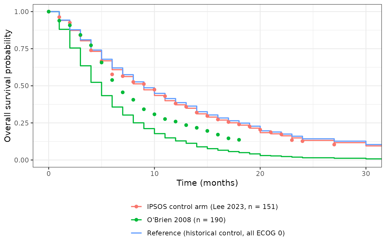
Model-predicted overall-survival curves (lines) against the digitised Kaplan-Meier data the model was fitted to (points). Replicates the per-trial fits of Chen 2026 Figure S2.
The IPSOS control arm – the arm the whole analysis is about – is described closely by the typical-value prediction.
pred_at <- function(lbl, times) {
  s <- sim[sim$label == lbl, ]
  idx <- match(times, s$time)
  stopifnot(!anyNA(idx))
  s$surv[idx]
}

ipsos_obs <- observed[observed$label == "IPSOS control arm (Lee 2023, n = 151)", ]
ipsos_chk <- dplyr::mutate(
  ipsos_obs,
  pred = pred_at("IPSOS control arm (Lee 2023, n = 151)", time),
  diff = pred - surv
)
stopifnot(nrow(ipsos_chk) == 26L)   # the gate must have rows to test

summary_stats <- c(
  median_abs_diff = median(abs(ipsos_chk$diff)),
  q90_abs_diff    = unname(quantile(abs(ipsos_chk$diff), 0.9)),
  max_abs_diff    = max(abs(ipsos_chk$diff))
)
round(summary_stats, 4)
#> median_abs_diff    q90_abs_diff    max_abs_diff
#>          0.0104          0.0384          0.0519

# Deterministic comparison (typical-value solve against fixed published data --
# no random draw on either side), so these bounds are reproducible across
# machines. They go red on a mis-transcribed decrement, a wrong ECOG
# coefficient, or a lost IPSOS indicator, each of which moves the curve by
# well over 0.05 in survival probability.
stopifnot(
  median(abs(ipsos_chk$diff)) < 0.03,
  quantile(abs(ipsos_chk$diff), 0.9) < 0.05
)
O’Brien 2008 is a different story, and the paper says so. Chen 2026 Section 3.2.3 notes that “the comparison between O’Brien and the IPSOS control shows that the IPSOS control was superior to O’Brien, despite having the same chemotherapy regimen of gemcitabine or vinorelbine”, and raises publication era or unmeasured heterogeneity as candidate explanations. In this model that gap is absorbed by the between-trial random effect: the arm survives markedly longer than its imputed all-ECOG-2 composition predicts.
obrien_obs <- observed[observed$label == "O'Brien 2008 (n = 190)", ]
obrien_chk <- dplyr::mutate(
  obrien_obs,
  pred = pred_at("O'Brien 2008 (n = 190)", time),
  diff = pred - surv
)
stopifnot(nrow(obrien_chk) == 19L)

# The typical-value prediction sits BELOW the observed curve throughout -- the
# model over-predicts this arm's hazard.
stopifnot(all(obrien_chk$diff[obrien_chk$time > 0] < 0))

# Size of the between-trial random effect required to reconcile the arm,
# estimated over months 6 to 18 where the curves are well separated.
w <- obrien_chk$time >= 6 & obrien_chk$time <= 18
eta_needed <- median(
  log(log(obrien_chk$surv[w]) / log(pred_at("Reference (historical control, all ECOG 0)",
                                            obrien_chk$time[w]))) - est("e_ecog23")
)
round(eta_needed, 3)
#> [1] -0.418
round(eta_needed / between_trial_sd, 2)
#> [1] -1.62

# Roughly a 2-standard-deviation trial: unusual but inside the between-trial
# distribution the model estimates, and consistent with the paper singling this
# study out. A loose bound, because the claim being made is only "large but not
# impossible".
stopifnot(eta_needed < 0, abs(eta_needed / between_trial_sd) > 1,
          abs(eta_needed / between_trial_sd) < 3.5)
Between-trial prediction interval
Chen 2026 Figure 3 compares the IPSOS control arm against the
prediction range of historical trials. The equivalent here is
the between-trial distribution of the reference curve:
log(HR) is normal with standard deviation 0.257, so the 90%
prediction band for a new historical all-ECOG-0 trial arm is available
in closed form and needs no simulation.
z90 <- qnorm(0.95)
band <- data.frame(
  time = grid,
  ref  = pred_at("Reference (historical control, all ECOG 0)", grid)
) |>
  dplyr::mutate(
    lower = ref^exp( z90 * between_trial_sd),
    upper = ref^exp(-z90 * between_trial_sd)
  )

ipsos_pred <- data.frame(
  time = grid,
  surv = pred_at("IPSOS control arm (Lee 2023, n = 151)", grid)
)

# Ordering is structural, not stochastic: exp(+z*sd) > 1 shortens survival.
stopifnot(all(band$lower <= band$ref + 1e-12),
          all(band$upper >= band$ref - 1e-12))
ggplot2::ggplot(band, ggplot2::aes(time)) +
  ggplot2::geom_ribbon(
    ggplot2::aes(ymin = lower, ymax = upper),
    fill = "grey70", alpha = 0.5
  ) +
  ggplot2::geom_step(ggplot2::aes(y = ref, linetype = "Historical reference (ECOG 0)"),
                     linewidth = 0.7) +
  ggplot2::geom_step(
    data = ipsos_pred,
    ggplot2::aes(time, surv, linetype = "IPSOS control arm"),
    linewidth = 0.7, colour = "firebrick"
  ) +
  ggplot2::coord_cartesian(xlim = c(0, 36), ylim = c(0, 1)) +
  ggplot2::labs(x = "Time (months)", y = "Overall survival probability",
                linetype = NULL) +
  ggplot2::theme_bw() +
  ggplot2::theme(legend.position = "bottom")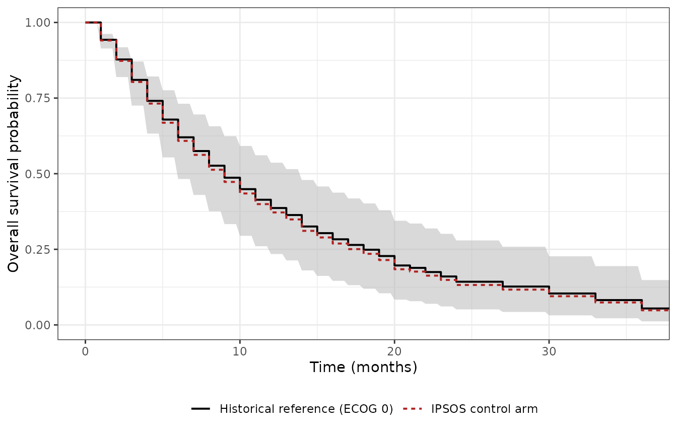
IPSOS control arm against the 90% between-trial prediction band for a historical all-ECOG-0 control arm. Analogous to Chen 2026 Figure 3.
A simulated cohort of trial arms reproduces the same band, and
confirms that eta_study is wired into log(HR)
rather than being inert.
n_arms <- 200L
rxode2::rxSetSeed(20260912)
cohort_ev <- do.call(rbind, lapply(seq_len(n_arms), function(i) {
  data.frame(
    id = i, time = knots, evid = 0L, amt = NA_real_,
    PS_ECOG_1_PCT = 0, PS_ECOG_2_PCT = 0, PS_ECOG_3_PCT = 0,
    TRT_IPSOS_CONTROL = 0
  )
}))
cohort <- rxode2::rxSolve(mod, cohort_ev, returnType = "data.frame")

# The random effect must actually vary between arms.
arm_log_hr <- cohort |>
  dplyr::distinct(id, lhr) |>
  dplyr::pull(lhr)
stopifnot(length(arm_log_hr) == n_arms, stats::sd(arm_log_hr) > 0)

round(c(mean = mean(arm_log_hr), sd = stats::sd(arm_log_hr)), 3)
#>  mean    sd
#> 0.013 0.253

# A 200-draw sample standard deviation has about a 5% relative standard error,
# so this is a deliberately wide envelope around the nominal 0.257 rather than
# a bound tightened to one observed run (see the CI-reproducibility note in
# the package vignette conventions).
stopifnot(abs(mean(arm_log_hr)) < 0.1,
          stats::sd(arm_log_hr) > 0.18, stats::sd(arm_log_hr) < 0.36)
Assumptions and deviations
-
Between knots the curve is held flat. The source
likelihood evaluates the reference curve only at the 30 knot times, so
the model as fitted says nothing about intermediate times. The packaged
model holds
surv0constant from each knot until the next, which is both the conservative reading and what a Kaplan-Meier curve is. Times between 24 and 27 months therefore report the 24-month value, and so on for the wider late knots. - Support is 1 to 48 months. The month 42-48 decrement was fixed to zero in the source control stream, so the reference curve is flat over that span and the model carries no information beyond 48 months. Extrapolating past 48 months returns the 42-month value and should not be treated as a prediction.
-
The random effect is between-trial, not
between-subject.
eta_studyis an MBMA variance component describing how far one trial arm’s whole survival curve sits from the model. Simulating it produces a distribution of trial arms, not of patients; this model cannot generate individual-subject event times. -
No residual error is encoded. Chen 2026 maximises a
user-supplied binomial
-2LLover per-interval death counts, with no$SIGMAin the control stream, so there is no residual-error parameter to carry and no observation endpoint is declared. The weight columnWTused in that likelihood is a fitting device and has no role in simulation. -
ECOG 2 and ECOG 3 share one coefficient, matching
COVECOG2*(PS2+PS3)/100in the source control stream. The two are kept as separate covariate columns because the source dataset carries them apart. - Arm-level ECOG percentages are partly imputed. Chen 2026 imputed 30 ECOG percentages, first by mapping Karnofsky Performance Scores and otherwise by splitting composite ECOG categories with a logistic regression calibrated on studies with similar entry criteria. O’Brien 2008 carries an imputed 100% ECOG 2, which is the largest single driver of its predicted hazard ratio and a plausible contributor to the misfit shown above.
- Only Model 010 is packaged. See Errata for why the paper’s other models are not reproducible from the published material.
- Digitisation and censoring. The database was built by digitising published Kaplan-Meier curves at monthly intervals with Engauge Digitizer 12.1. Censoring tick marks could not be recovered, which the authors note may over-weight later time points; they mitigated it by trimming curve tails where fewer than 10 patients remained at risk or survival fell below 0.1.
Errata
-
The distributed control stream is not Model 010.
The Supporting Information file
psp470197-sup-0002-Supinfo2.ctlis referenced by the Figure S2 caption as “the control file … for the final model (model010)”, but its$PREDblock fixes the ECOG effects to the external Lee meta-analysis values (LOG(1.43)andLOG(2.71)), adds fixed Stage IV and sex effects that appear in no reported model, and carriesATEZOas0 FIXwith no IPSOS control term. Model 010 by definition estimates the ECOG effects (Table 3) and retains an IPSOS control effect. The file is therefore a different run – structurally closest to Model 007b. It is used here only as the authority for the model form (the logit random walk, theS^exp(log HR)rescaling, the conditional-death-probability likelihood, and the0 FIXfinal decrement); every parameter value comes from Table S8, which is explicitly headed “Final Model Parameters (mod010)” and which reproduces all three of the Table 3 Model 010 hazard ratios exactly. - The paper’s headline hazard ratios come from Model 041, not Model 010. The Abstract, Discussion and Conclusions quote HR 0.543 (95% CI 0.435 to 0.677) for the IPSOS control arm and HR 0.418 (95% CI 0.335 to 0.522) for the IPSOS atezolizumab arm. Both are Model 041 (Table 4), which adds the atezolizumab arm to the dataset and estimates a second treatment effect. Model 010’s corresponding IPSOS control estimate is 0.531 (95% CI 0.424 to 0.664). Only Model 010 has a published reference survival curve – Table S8 is the paper’s only complete parameter listing – so the atezolizumab effect is not packaged. Grafting the Model 041 atezolizumab hazard ratio onto the Model 010 reference curve would mix parameters from two different fits, and is deliberately not done.
- Abstract-to-Discussion inconsistency in the IPSOS control confidence interval. The Abstract reports 0.543 (95% CI 0.435 to 0.677) while Table 4 reports the same point estimate with 95% CI 0.436 to 0.676. The discrepancy is in the last digit of each bound and does not affect the model.
-
Table S8 abbreviation gloss. The Table S8 footnote
expands RSE as “residual standard error”, but its own Note defines the
column as
SE / Estimate * 100%, i.e. the relative standard error. The values in the column are relative standard errors; the abbreviation list is wrong. - Table 4 is unreadable in the PMC text conversion. The open-access PMC rendering of Table 4 collapses its columns into a single cell, losing the model-to-hazard-ratio mapping. The values used here were read from the laid-out PDF, where the table is intact.
-
Supporting Information. The Supporting Information
is published with the open-access article (PMC12909276). It comprises
Supinfo1(the NONMEM analysis dataset),Supinfo2(the control stream discussed above) andSupinfo3(Tables S1 to S8 and Figures S1 to S3).