IL-6-mediated CYP3A suppression (Chen 2024)
Source:vignettes/articles/Chen_2024_interleukin6_cyp3a_pbpk.Rmd
Chen_2024_interleukin6_cyp3a_pbpk.Rmd
library(nlmixr2lib)
library(rxode2)
library(PKNCA)
library(dplyr)
library(ggplot2)

# readModelDb() returns the model *function*; rxode2() builds the rxUi object,
# which is what exposes `$omega` for the population simulation below.
mod <- rxode2::rxode2(readModelDb("Chen_2024_interleukin6_cyp3a_pbpk"))
Scope of this model
Chen 2024 built a Simcyp Simulator V17 model to ask whether the transient interleukin-6 (IL-6) elevation that follows mosunetuzumab dosing suppresses CYP3A enough to matter for co-administered CYP3A substrates. The published work has three layers, and only the first two are reproducible from the published sources:
| Layer | Content | In this model? |
|---|---|---|
| A | IL-6 disposition (CL 2.8 L/h, Vss 0.43 L/kg), driven by hypothetical IL-6 infusions | Yes, reduced to one compartment |
| B | CYP3A enzyme turnover and IL-6 suppression in liver and gut (Appendix S1 Equation 1) | Yes, in full |
| C | Midazolam and simvastatin exposure ratios | No |
Layer C used unmodified proprietary Simcyp V17 compound files. Tables
S1 and S2 give compound-file inputs only: the
Vmax/Km values are expressed per pmol of
isoform and cannot be scaled to an in vivo clearance without MPPGL,
liver weight, hepatic blood flow, and Qgut, none of which
are reported. Every exposure-ratio result in the paper (Tables 2, 3, S3,
S4) is a Layer C output and is therefore outside the scope of this file.
What this model does provide is the upstream quantity that
drives all of them: the time course of CYP3A activity.
Note also that mosunetuzumab itself is never modelled. It enters the published work only through hypothetical IL-6 infusion amounts hand-calibrated to reproduce the observed IL-6 profile.
Population
knitr::kable(
  data.frame(
    Field = c("Species", "Subjects", "Disease state", "IL-6 source regimen"),
    Value = c(
      "human",
      "212 (observed IL-6 data)",
      "relapsed/refractory non-Hodgkin lymphoma",
      "mosunetuzumab 1/2/60 mg IV, cycle 1 days 1/8/15"
    )
  )
)| Field | Value |
|---|---|
| Species | human |
| Subjects | 212 (observed IL-6 data) |
| Disease state | relapsed/refractory non-Hodgkin lymphoma |
| IL-6 source regimen | mosunetuzumab 1/2/60 mg IV, cycle 1 days 1/8/15 |
Observed plasma IL-6 concentration-time profiles come from 212 patients in dose-expansion cohort B11 of study GO29781 (NCT02500407), measured by Quantikine ELISA over a validated range of 3.13 to 300 pg/mL (Appendix S1). The CYP3A suppression layer was verified against two independent cohorts: rheumatoid arthritis patients with chronically elevated IL-6, and patients recovering from hip surgery with transient IL-6 elevation.
Source trace
Every value in ini(), with the location it came
from.
| Parameter | Value | Source |
|---|---|---|
| lcl | 2.8 L/h | Table 1 and Methods (CL determined top-down) |
| lvc | 0.43 L/kg | Table 1, minimal PBPK distribution model |
| emin | 0.217 | Table 1 footnote (Indmax 0.217); Appendix S1 donor table geometric mean 21.7% |
| ec50 | 43.7 pg/mL | Table 1; Appendix S1 donor table geometric mean |
| kdeg_liver | 0.0193 /h | Table 1 (Simcyp library); restated in Appendix S1 |
| kdeg_gut | 0.03 /h | Table 1, CYP3A4 turnover rate in gut |
| bl_enzyme_3a4_liver | 137 pmol/mg protein | Table 1, CYP3A4 in liver in healthy volunteers |
| bl_enzyme_3a4_gut | 66.2 nmol/small intestine | Table 1, CYP3A4 in gut in healthy volunteers |
| etalcl | 1.6094 | Table 1, CLint 200 %CV; log(1 + 2.00^2) |
| etalvc | 0.6931 | Table 1, Vss 100 %CV; log(1 + 1.00^2) |
| propSd | 0 (fixed) | not reported (simulation-only source) |
| Equation 1 | enzyme turnover with IL-6 suppression | Appendix S1 Equation 1, attributed to Machavaram 2013 |
The two in vitro suppression constants are geometric means over five human hepatocyte donors (Dickmann 2011), tabulated per donor in Appendix S1. Both reproduce exactly from the donor values:
donors <- data.frame(
  donor = c("Hu1001", "Hu8064", "Hu1146", "Hu1150", "Hu4151"),
  ec50 = c(4.23, 176, 59.7, 43.1, 82.8),
  emin_pct = c(41.7, 21.1, 10.7, 29.7, 17.1)
)
geomean <- function(x) exp(mean(log(x)))
data.frame(
  Constant = c("EC50 (pg/mL)", "Emin (%)"),
  Recomputed = round(c(geomean(donors$ec50), geomean(donors$emin_pct)), 2),
  Published = c(43.7, 21.7)
) |>
knitr::kable()| Constant | Recomputed | Published |
|---|---|---|
| EC50 (pg/mL) | 43.66 | 43.7 |
| Emin (%) | 21.67 | 21.7 |
Dimensional analysis
Mechanistic models mix per-kg volumes, mass amounts, and fractional rate constants, so every ODE term is checked explicitly.
| Term | Units | Result |
|---|---|---|
central |
mg | state |
vc = exp(lvc) * WT |
(L/kg) * kg = L | volume |
cl / vc * central |
(L/h) / L * mg = mg/h | matches d(central)/dt |
Cc = central / vc * 1e6 |
mg/L * (pg/mL)/(mg/L) = pg/mL | matches EC50 units |
fsupp |
unitless (both emin and the Michaelis term are
unitless) |
scalar |
kdeg_liver * bl_enzyme_3a4_liver * fsupp |
(1/h) * (pmol/mg) = pmol/mg/h | matches d(enzyme_3a4_liver)/dt |
kdeg_liver * enzyme_3a4_liver |
(1/h) * (pmol/mg) = pmol/mg/h | matches |
The single non-obvious conversion is 1e6: amounts are in
mg and volumes in L, so central / vc is mg/L, and 1 mg/L =
1e6 pg/mL. EC50 and every published IL-6 concentration are in pg/mL, so
this factor must be present for the suppression term to be evaluated on
the right scale.
Model structure
IL-6 is a one-compartment intravenous model. CYP3A activity in each tissue follows Appendix S1 Equation 1:
The bracketed term is the fractional synthesis rate: it equals 1 when
no IL-6 is present and falls toward Emin = 0.217 as IL-6
rises. Each enzyme pool therefore relaxes toward
ENZ0 * fsupp with a time constant 1/kdeg.
Because the gut kdeg (0.03 /h) is faster than the hepatic
kdeg (0.0193 /h), gut CYP3A both responds faster and
reaches a deeper nadir under a transient IL-6 pulse. That difference is
the only thing distinguishing the two tissues, and it is what the Figure
4d check below tests.
WT_REF <- 70

# Typical-value (no IIV) version of the model.
tv <- rxode2::zeroRe(mod)

# Solve a typical subject over an event table, returning a data frame.
solve_tv <- function(ev, tmax, by = 0.25) {
  ev <- ev |> rxode2::et(seq(0, tmax, by = by), cmt = "central")
  rxode2::rxSolve(
    tv, ev,
    params = c(WT = WT_REF),
    omega = NA,
    returnType = "data.frame"
  )
}

# A zero-order IL-6 infusion of `amt` mg delivered over `dur` hours.
infusion <- function(amt, dur, time = 0) {
  rxode2::et(amt = amt, rate = amt / dur, time = time, cmt = "central")
}

pct_reduction <- function(x) 100 * (1 - x)
Check 1: steady state with no IL-6
With no IL-6 present, fsupp is exactly 1 and each enzyme
pool must hold at its baseline abundance indefinitely. This confirms the
production and loss terms balance and that the initial conditions are
consistent with the ODEs.
ss <- solve_tv(rxode2::et(amt = 0, time = 0, cmt = "central"), tmax = 1000, by = 5)

data.frame(
  Pool = c("liver", "gut"),
  Baseline = c(137, 66.2),
  `Min over 1000 h` = c(min(ss$enzyme_3a4_liver), min(ss$enzyme_3a4_gut)),
  `Max over 1000 h` = c(max(ss$enzyme_3a4_liver), max(ss$enzyme_3a4_gut)),
  check.names = FALSE
) |>
knitr::kable(digits = 6)| Pool | Baseline | Min over 1000 h | Max over 1000 h |
|---|---|---|---|
| liver | 137.0 | 137.0 | 137.0 |
| gut | 66.2 | 66.2 | 66.2 |
stopifnot(
  all.equal(range(ss$enzyme_3a4_liver), c(137, 137), tolerance = 1e-8),
  all.equal(range(ss$enzyme_3a4_gut), c(66.2, 66.2), tolerance = 1e-8),
  all.equal(range(ss$Cc), c(0, 0), tolerance = 1e-12)
)
No drift: production kdeg * ENZ0 * 1 exactly cancels
loss kdeg * ENZ0.
Check 2: perturbation recovery
Displacing each enzyme pool away from baseline, with no IL-6 present,
must send it monotonically back to baseline at rate kdeg.
This confirms kdeg acts as a recovery rate constant and not
merely as a scale factor on the synthesis term.
The displacement is applied with evid = 5 (replacement)
dosing events on the enzyme compartments, following the pattern used by
vanErp_2010_sunitinib. Note that the inits
argument to rxSolve() would not work here: the
model body sets
enzyme_3a4_liver(0) <- bl_enzyme_3a4_liver, and a
model-body initial condition takes precedence over inits,
so the states would silently stay at baseline and the check would pass
vacuously.
recover <- function(f_liver, f_gut) {
  ev <- rxode2::et(amt = f_liver * 137, cmt = "enzyme_3a4_liver", time = 0, evid = 5) |>
    rxode2::et(amt = f_gut * 66.2, cmt = "enzyme_3a4_gut", time = 0, evid = 5) |>
    rxode2::et(seq(0, 600, by = 1), cmt = "central")
  rxode2::rxSolve(
    tv, ev,
    params = c(WT = WT_REF),
    omega = NA,
    returnType = "data.frame"
  )
}

lo <- recover(0.5, 0.5)
hi <- recover(1.5, 1.5)

# The displacement must actually have happened, or the check is vacuous.
stopifnot(
  abs(lo$enzyme_3a4_liver[1] - 0.5 * 137) < 1e-6,
  abs(hi$enzyme_3a4_liver[1] - 1.5 * 137) < 1e-6
)

# Recovery half-life should equal log(2)/kdeg for each tissue.
half_life <- function(d, state, bl) {
  gap <- abs(d[[state]] - bl)
  d$time[which.min(abs(gap - gap[1] / 2))]
}

data.frame(
  Pool = c("liver", "gut"),
  `Observed recovery t1/2 (h)` = c(
    half_life(lo, "enzyme_3a4_liver", 137),
    half_life(lo, "enzyme_3a4_gut", 66.2)
  ),
  `log(2)/kdeg (h)` = round(log(2) / c(0.0193, 0.03), 1),
  check.names = FALSE
) |>
knitr::kable(digits = 1)| Pool | Observed recovery t1/2 (h) | log(2)/kdeg (h) |
|---|---|---|
| liver | 36 | 35.9 |
| gut | 23 | 23.1 |
stopifnot(
  abs(tail(lo$enzyme_3a4_liver, 1) - 137) < 0.01,
  abs(tail(hi$enzyme_3a4_liver, 1) - 137) < 0.01,
  abs(tail(lo$enzyme_3a4_gut, 1) - 66.2) < 0.01,
  abs(tail(hi$enzyme_3a4_gut, 1) - 66.2) < 0.01
)
bind_rows(
  lo |> mutate(start = "50% of baseline"),
  hi |> mutate(start = "150% of baseline")
) |>
  select(time, start, liver = cyp3aLiver, gut = cyp3aGut) |>
  tidyr::pivot_longer(c(liver, gut), names_to = "tissue", values_to = "activity") |>
  ggplot(aes(time, activity, colour = tissue, linetype = start)) +
  geom_hline(yintercept = 1, linetype = "dotted") +
  geom_line() +
  labs(x = "Time (h)", y = "CYP3A activity (fraction of baseline)",
       colour = "Tissue", linetype = "Initial value") +
  theme_bw()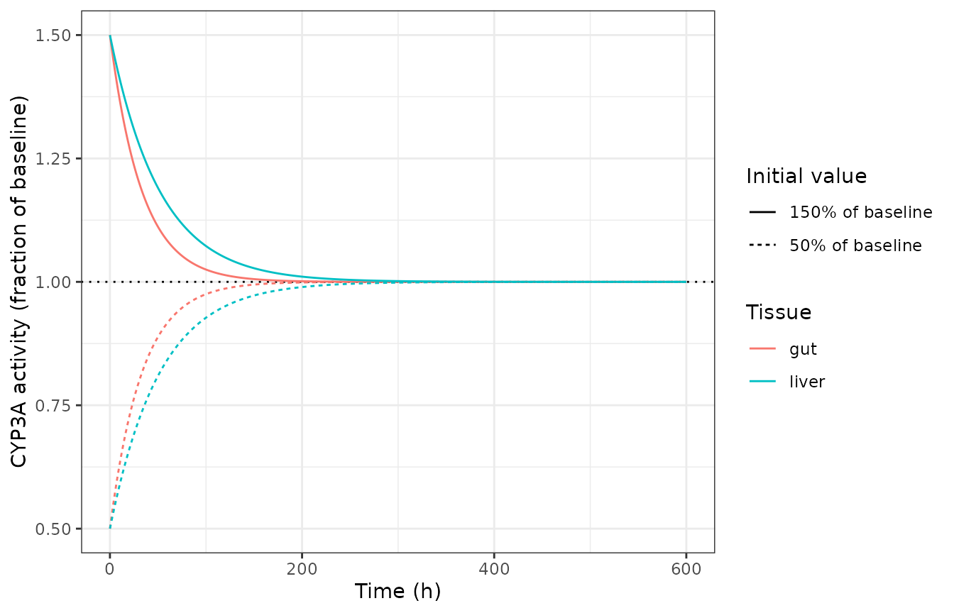
Perturbation recovery of both CYP3A pools toward baseline with no IL-6 present.
Hepatic recovery is slower than gut recovery, in the ratio of the two
kdeg values, as expected.
Check 3: clamped IL-6 (replicates Figure 4c)
Figure 4c reports CYP3A suppression at the constant IL-6 concentrations seen in rheumatoid arthritis patients: 50 and 100 pg/mL. The published values are 40% to 52% reduction in liver and 41% to 54% in gut across that range.
At steady state the enzyme ODE gives activity exactly equal to
fsupp, so this check has a closed form that the simulation
must match:
fsupp <- function(C, emin = 0.217, ec50 = 43.7) 1 + (emin - 1) * C / (ec50 + C)
data.frame(
  `IL-6 (pg/mL)` = c(50, 100),
  `Closed-form reduction (%)` = round(pct_reduction(fsupp(c(50, 100))), 1),
  `Published liver (%)` = c(40, 52),
  `Published gut (%)` = c(41, 54),
  check.names = FALSE
) |>
knitr::kable()| IL-6 (pg/mL) | Closed-form reduction (%) | Published liver (%) | Published gut (%) |
|---|---|---|---|
| 50 | 41.8 | 40 | 41 |
| 100 | 54.5 | 52 | 54 |
To reproduce it dynamically, IL-6 is clamped by a 21-day zero-order
infusion at the rate that holds the target concentration
(rate = Css * CL).
clamp <- function(Css, days = 21) {
  rate <- Css * 1e-6 * 2.8              # mg/h; Css pg/mL -> mg/L is 1e-6
  d <- solve_tv(infusion(rate * days * 24, days * 24), tmax = days * 24, by = 1)
  data.frame(
    Css_target = Css,
    Css_sim = tail(d$Cc, 1),
    liver_pct = pct_reduction(tail(d$cyp3aLiver, 1)),
    gut_pct = pct_reduction(tail(d$cyp3aGut, 1)),
    liver_abundance = tail(d$enzyme_3a4_liver, 1),
    gut_abundance = tail(d$enzyme_3a4_gut, 1)
  )
}

clamped <- bind_rows(clamp(50), clamp(100))

clamped |>
  transmute(
    `Target IL-6 (pg/mL)` = Css_target,
    `Simulated IL-6 (pg/mL)` = round(Css_sim, 2),
    `Liver reduction (%)` = round(liver_pct, 1),
    `Gut reduction (%)` = round(gut_pct, 1)
  ) |>
knitr::kable()| Target IL-6 (pg/mL) | Simulated IL-6 (pg/mL) | Liver reduction (%) | Gut reduction (%) |
|---|---|---|---|
| 50 | 50 | 41.8 | 41.8 |
| 100 | 100 | 54.5 | 54.5 |
stopifnot(
  abs(clamped$Css_sim - clamped$Css_target) < 0.05,
  abs(clamped$liver_pct - c(41.8, 54.5)) < 0.2
)
Both reproduce the published ranges. The liver and gut values are
identical here because at steady state kdeg cancels out of
the enzyme equation; the tissues differ only in their dynamics,
which Check 4 exercises.
The rheumatoid-arthritis abundance target
The paper’s verification logic is stated numerically in Methods: Simcyp’s rheumatoid-arthritis population assumes CYP3A4 abundances 40% below healthy volunteers, namely 82.2 pmol/mg protein in liver and 40.0 nmol/small intestine in gut. The question the authors posed was whether their IL-6 model, driven only by in vitro suppression constants, predicts those abundances. It does:
ra <- clamped[clamped$Css_target == 50, ]
predicted <- c(ra$liver_abundance, ra$gut_abundance)
ra_target <- c(82.2, 40.0)

data.frame(
  Pool = c("liver", "gut"),
  Predicted = round(predicted, 1),
  `Simcyp RA population value` = ra_target,
  `% difference` = round(100 * (predicted / ra_target - 1), 1),
  check.names = FALSE
) |>
knitr::kable()| Pool | Predicted | Simcyp RA population value | % difference |
|---|---|---|---|
| liver | 79.8 | 82.2 | -3.0 |
| gut | 38.5 | 40.0 | -3.6 |
Within about 3% on both tissues, from a model whose suppression constants were measured in hepatocyte culture and never fitted to the rheumatoid-arthritis data. This is the single strongest confirmation that the enzyme layer was transcribed correctly.
Check 4: transient IL-6 after hip surgery (replicates Figure 4d)
This is the check that tests the two kdeg values,
because a transient pulse resolves the tissues that a steady-state clamp
cannot. Table 1 footnote e gives the hypothetical IL-6 dose used for
this cohort: 0.02 mg infused over 24 h. Figure 4d reports roughly 31%
hepatic and 42% intestinal reduction, with maximum suppression on days 2
to 3, about 24 h after the peak IL-6 concentration.
hip <- solve_tv(infusion(0.02, 24), tmax = 240, by = 0.25)

summ <- data.frame(
  Quantity = c(
    "Peak IL-6 (pg/mL)", "Time of peak IL-6 (h)",
    "Max liver reduction (%)", "Time of max liver reduction (h)",
    "Max gut reduction (%)", "Time of max gut reduction (h)"
  ),
  Simulated = c(
    round(max(hip$Cc), 1), hip$time[which.max(hip$Cc)],
    round(pct_reduction(min(hip$cyp3aLiver)), 1),
    hip$time[which.min(hip$cyp3aLiver)],
    round(pct_reduction(min(hip$cyp3aGut)), 1),
    hip$time[which.min(hip$cyp3aGut)]
  ),
  Published = c(
    "not reported", "not reported",
    "~31", "day 2-3",
    "~42", "day 2-3"
  )
)
knitr::kable(summ)| Quantity | Simulated | Published |
|---|---|---|
| Peak IL-6 (pg/mL) | 265.70 | not reported |
| Time of peak IL-6 (h) | 24.00 | not reported |
| Max liver reduction (%) | 32.50 | ~31 |
| Time of max liver reduction (h) | 47.00 | day 2-3 |
| Max gut reduction (%) | 41.20 | ~42 |
| Time of max gut reduction (h) | 42.25 | day 2-3 |
p_conc <- ggplot(hip, aes(time, Cc)) +
  geom_line(colour = "steelblue") +
  labs(x = "Time (h)", y = "IL-6 (pg/mL)", title = "IL-6 (Figure 4b)") +
  theme_bw()

p_enz <- hip |>
  select(time, liver = cyp3aLiver, gut = cyp3aGut) |>
  tidyr::pivot_longer(c(liver, gut), names_to = "tissue", values_to = "activity") |>
  ggplot(aes(time, activity, colour = tissue)) +
  geom_line() +
  scale_y_continuous(limits = c(0, 1)) +
  labs(x = "Time (h)", y = "CYP3A activity (fraction of baseline)",
       colour = "Tissue", title = "CYP3A activity (Figure 4d)") +
  theme_bw()

print(p_conc)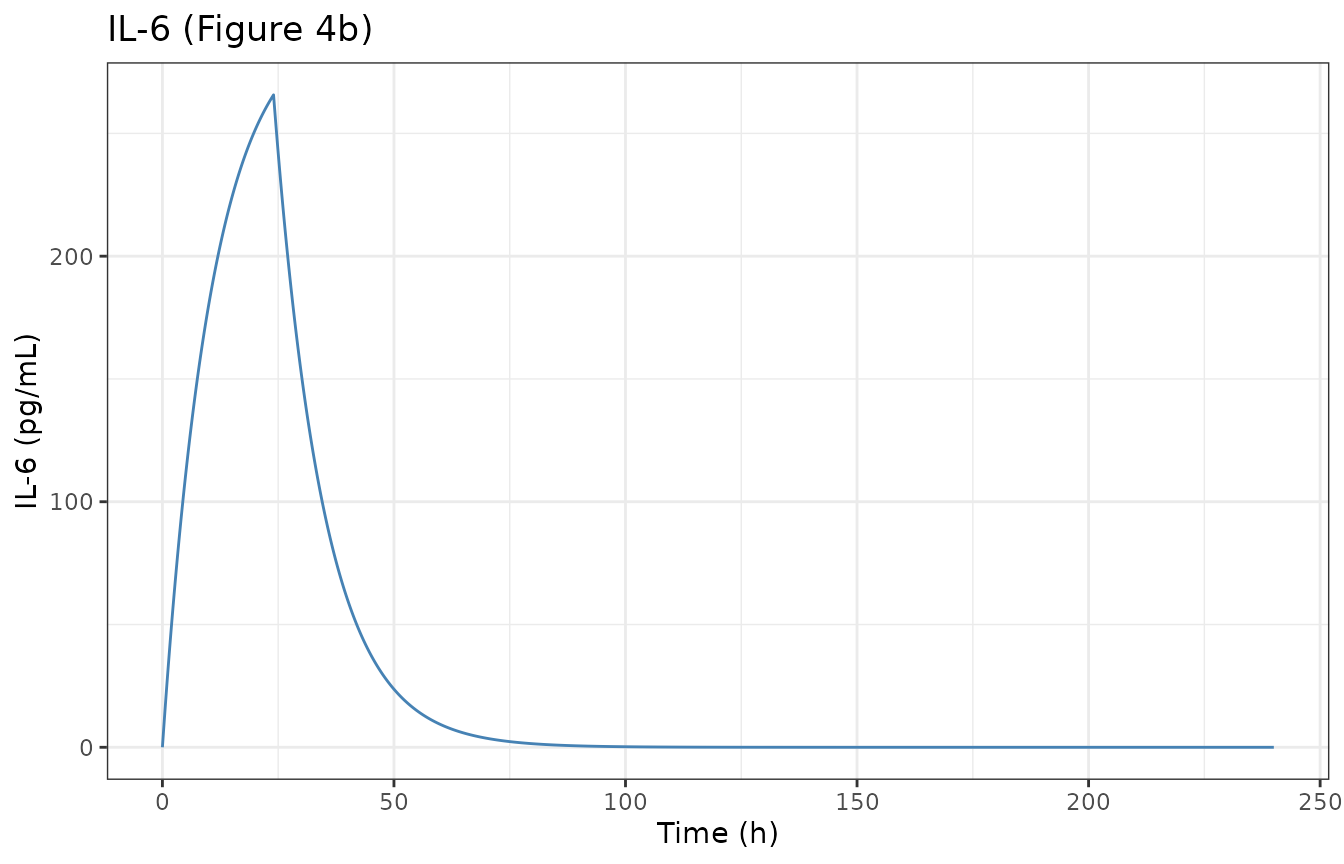
Replicates Figure 4b and 4d of Chen 2024: transient IL-6 elevation after hip surgery and the resulting CYP3A suppression in liver and gut.
print(p_enz)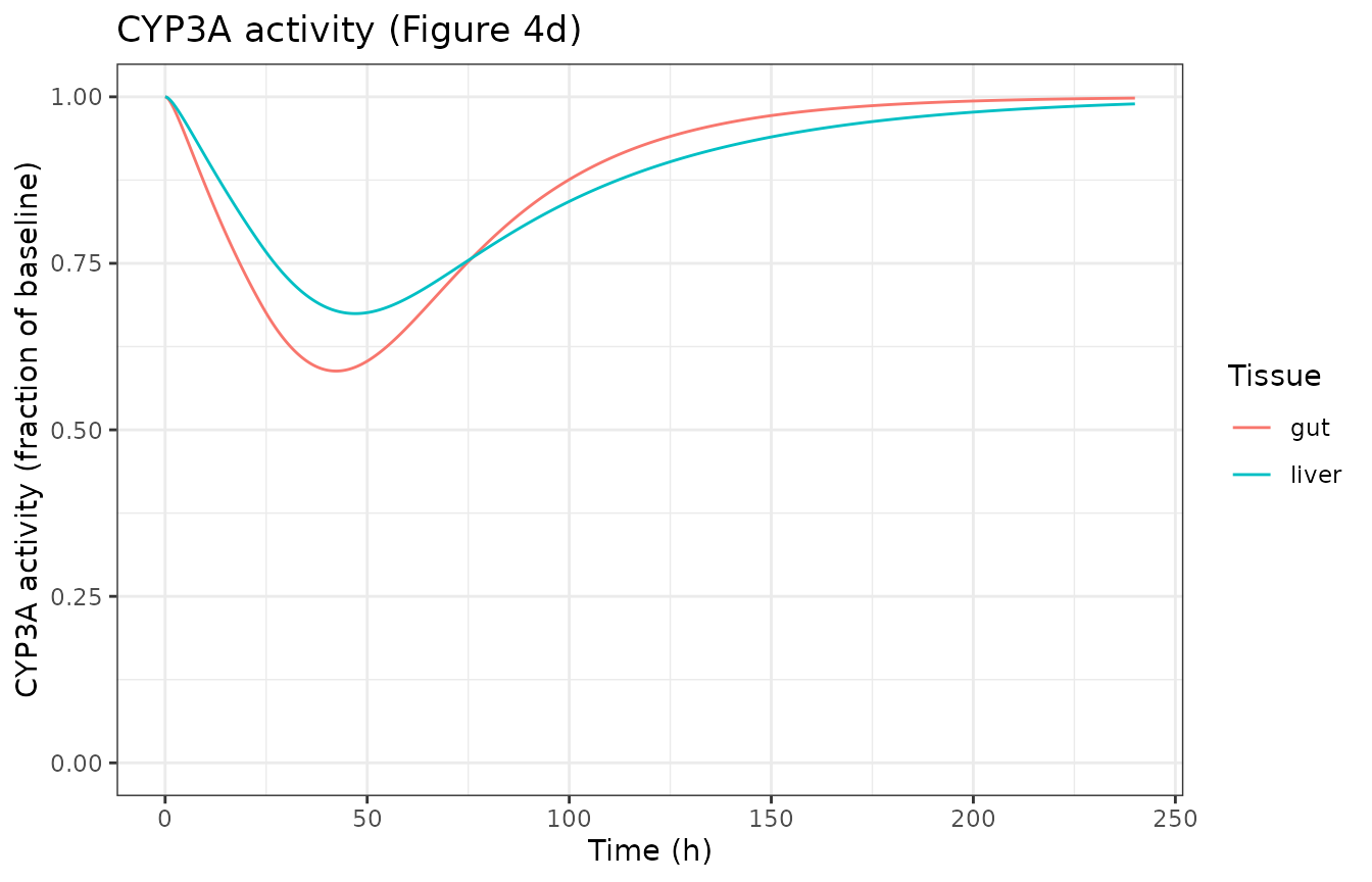
Replicates Figure 4b and 4d of Chen 2024: transient IL-6 elevation after hip surgery and the resulting CYP3A suppression in liver and gut.
The reproduction is close on both tissues (simulated about 32% liver
and 41% gut, against published values of about 31% and 42%), and the
ordering is correct: gut suppression is deeper and earlier than hepatic
suppression. Maximum suppression falls roughly 18 to 23 h after the IL-6
peak, matching the paper’s statement that it occurs about 24 h
post-peak. Nothing was tuned to achieve this: the dose, the duration,
both kdeg values, EC50, and Emin
are all as published.
Check 5: mosunetuzumab cycle 1 (replicates Figure 3)
Table 1 footnote c gives the hypothetical IL-6 doses used to reproduce the observed cycle-1 profile: 0.004, 0.0017, and 0.011 mg infused over 6, 6, and 13 h on days 1, 8, and 15.
ev_mos <- infusion(0.004,  6,  time = 0) |>
  rxode2::et(amt = 0.0017, rate = 0.0017 / 6,  time = 168, cmt = "central") |>
  rxode2::et(amt = 0.011,  rate = 0.011 / 13,  time = 336, cmt = "central")

mos <- solve_tv(ev_mos, tmax = 600, by = 0.25)
obs_peaks <- data.frame(
  time = c(6, 168 + 24, 336 + 24),
  Cc = c(152, 52.7, 160),
  label = c("C1D1", "C1D8", "C1D15")
)

ggplot(mos, aes(time, Cc)) +
  geom_line(colour = "steelblue") +
  geom_point(data = obs_peaks, aes(time, Cc), colour = "firebrick", size = 2) +
  labs(x = "Time (h)", y = "IL-6 (pg/mL)",
       title = "Simulated IL-6, with observed mean peaks (red)") +
  theme_bw()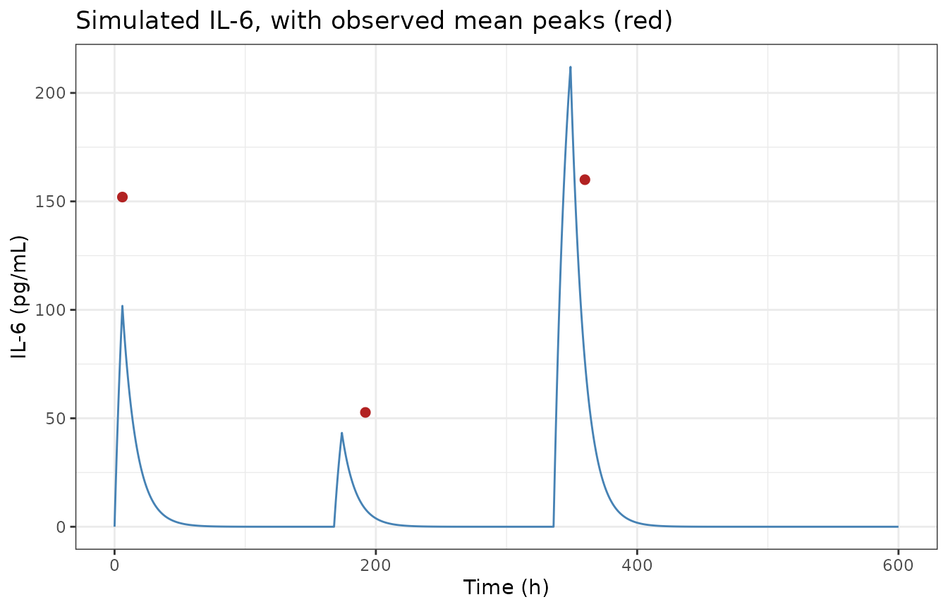
Replicates Figure 3 of Chen 2024: simulated IL-6 elevation (a) and CYP3A activity suppression (b) over cycle 1 at the 1/2/60 mg mosunetuzumab regimen.
mos |>
  select(time, liver = cyp3aLiver, gut = cyp3aGut) |>
  tidyr::pivot_longer(c(liver, gut), names_to = "tissue", values_to = "activity") |>
  ggplot(aes(time, activity, colour = tissue)) +
  geom_line() +
  scale_y_continuous(limits = c(0, 1)) +
  labs(x = "Time (h)", y = "CYP3A activity (fraction of baseline)",
       colour = "Tissue", title = "CYP3A activity suppression") +
  theme_bw()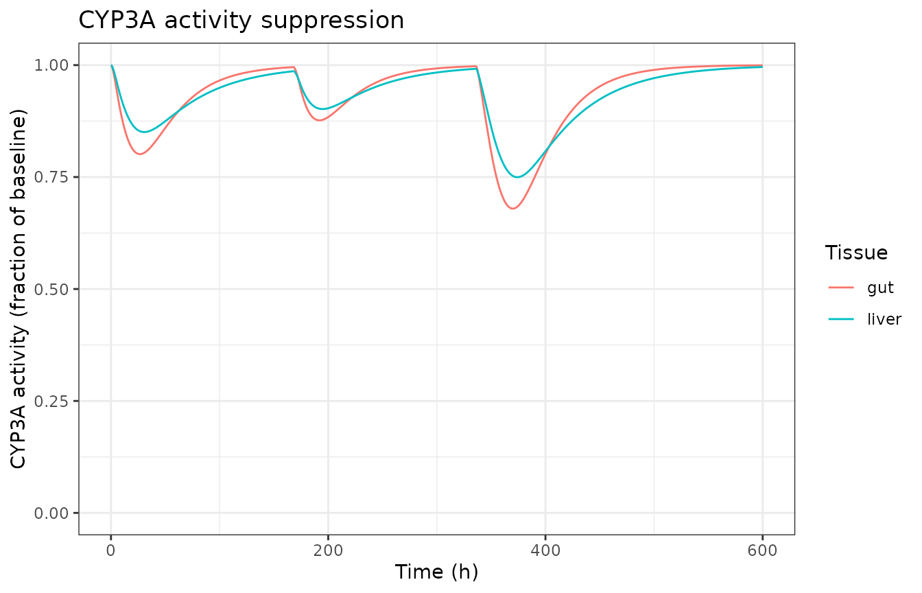
Replicates Figure 3 of Chen 2024: simulated IL-6 elevation (a) and CYP3A activity suppression (b) over cycle 1 at the 1/2/60 mg mosunetuzumab regimen.
windows <- list(C1D1 = c(0, 160), C1D8 = c(168, 330), C1D15 = c(336, 600))
per_dose <- lapply(names(windows), function(nm) {
  w <- windows[[nm]]
  s <- mos[mos$time >= w[1] & mos$time <= w[2], ]
  data.frame(
    Dose = nm,
    `Peak IL-6 (pg/mL)` = round(max(s$Cc), 1),
    `Liver reduction (%)` = round(pct_reduction(min(s$cyp3aLiver)), 1),
    `Gut reduction (%)` = round(pct_reduction(min(s$cyp3aGut)), 1),
    check.names = FALSE
  )
}) |>
  bind_rows()
knitr::kable(per_dose)| Dose | Peak IL-6 (pg/mL) | Liver reduction (%) | Gut reduction (%) |
|---|---|---|---|
| C1D1 | 101.8 | 14.9 | 19.9 |
| C1D8 | 43.3 | 9.8 | 12.3 |
| C1D15 | 212.0 | 25.0 | 32.0 |
The paper states that “up to 30% enzyme activity reduction was predicted at a mosunetuzumab dose level of 60 mg on C1D15.” The reduced model gives 25% hepatic reduction at C1D15. The shortfall traces to Layer A rather than Layer B: see the Cmax comparison below and the Errata.
Non-compartmental analysis of the IL-6 profiles
The paper reports observed mean IL-6 peak concentrations, so
PKNCA is used to extract the corresponding simulated
values. Because the IL-6 half-life (log(2) * Vss / CL,
about 7.4 h) is far shorter than the 7-day dosing interval, there is no
accumulation across the three doses, and each is simulated as an
independent single-dose profile.
single_dose <- function(amt, dur, label) {
  d <- solve_tv(infusion(amt, dur), tmax = 168, by = 0.25)
  d$treatment <- label
  d$id <- 1L
  d
}

nca_data <- bind_rows(
  single_dose(0.004,  6,  "C1D1"),
  single_dose(0.0017, 6,  "C1D8"),
  single_dose(0.011,  13, "C1D15")
) |>
  filter(!is.na(Cc))

dose_data <- data.frame(
  id = 1L,
  treatment = c("C1D1", "C1D8", "C1D15"),
  time = 0,
  amt = c(0.004, 0.0017, 0.011)
)

o_conc <- PKNCA::PKNCAconc(
  nca_data, Cc ~ time | treatment + id,
  concu = "pg/mL", timeu = "h"
)
o_dose <- PKNCA::PKNCAdose(
  dose_data, amt ~ time | treatment + id,
  doseu = "mg"
)

intervals <- data.frame(
  start = 0, end = Inf,
  cmax = TRUE, tmax = TRUE, half.life = TRUE, aucinf.obs = TRUE
)
res <- PKNCA::pk.nca(PKNCA::PKNCAdata(o_conc, o_dose, intervals = intervals))

sim_nca <- as.data.frame(res)
reference <- data.frame(
  treatment = c("C1D1", "C1D8", "C1D15"),
  cmax = c(152, 52.7, 160),
  tmax = c(6, 24, 24)
)

tbl <- nlmixr2lib::ncaComparisonTable(
  simulated = sim_nca,
  reference = reference,
  by = "treatment",
  params = c("cmax", "tmax"),
  units = c(cmax = "pg/mL", tmax = "h")
)
knitr::kable(tbl)| NCA parameter | treatment | Reference | Simulated | % diff |
|---|---|---|---|---|
| Cmax (pg/mL) | C1D1 | 152 | 102 | -33.0%* |
| Cmax (pg/mL) | C1D8 | 52.7 | 43.3 | -17.9% |
| Cmax (pg/mL) | C1D15 | 160 | 212 | +32.5%* |
| Tmax (h) | C1D1 | 6 | 6 | +0.0% |
| Tmax (h) | C1D8 | 24 | 6 | -75.0%* |
| Tmax (h) | C1D15 | 24 | 13 | -45.8%* |
attr(tbl, "footnote")
#> [1] "* differs from reference by more than ±20%."
The reference column here is the observed clinical mean, not the paper’s own simulated value; Chen 2024 never tabulates its simulated IL-6 peaks. The comparison is therefore a check on the reduced Layer A, and it does not pass cleanly. This is expected and is discussed in the Errata: it is the known, declared limitation of reducing the Simcyp minimal-PBPK topology to one compartment, and it does not propagate into the enzyme layer, which is validated against concentration directly in Checks 3 and 4.
Sensitivity: 95th-percentile IL-6
Table 1 footnote c also gives the hypothetical doses used to drive the sensitivity analysis at roughly the 95th percentile of observed IL-6: 0.0135, 0.007, and 0.045 mg over 6, 6, and 25 h.
ev_hi <- infusion(0.0135, 6, time = 0) |>
  rxode2::et(amt = 0.007, rate = 0.007 / 6,  time = 168, cmt = "central") |>
  rxode2::et(amt = 0.045, rate = 0.045 / 25, time = 336, cmt = "central")

hi_sim <- solve_tv(ev_hi, tmax = 600, by = 0.25)

data.frame(
  Scenario = c("Mean IL-6", "95th-percentile IL-6"),
  `Peak IL-6 (pg/mL)` = round(c(max(mos$Cc), max(hi_sim$Cc)), 1),
  `Max liver reduction (%)` = round(
    pct_reduction(c(min(mos$cyp3aLiver), min(hi_sim$cyp3aLiver))), 1
  ),
  `Max gut reduction (%)` = round(
    pct_reduction(c(min(mos$cyp3aGut), min(hi_sim$cyp3aGut))), 1
  ),
  check.names = FALSE
) |>
knitr::kable()| Scenario | Peak IL-6 (pg/mL) | Max liver reduction (%) | Max gut reduction (%) |
|---|---|---|---|
| Mean IL-6 | 212 | 25.0 | 32 |
| 95th-percentile IL-6 | 580 | 40.1 | 49 |
Raising IL-6 roughly threefold deepens hepatic suppression from 25%
to about 40%. The saturating shape of the suppression term is why the
paper concludes that “varying peak IL-6 concentrations could have only a
marginal effect, especially once maximum inhibition has been reached”:
once IL-6 is well above EC50 = 43.7 pg/mL, further
increases move fsupp very little.
Population simulation
Table 1 reports the between-subject variability used for the mosunetuzumab application: 200 %CV on clearance and 100 %CV on Vss, deliberately inflated above the Simcyp defaults so the simulated 5th-95th percentile band would cover the observed IL-6 data. These are the values encoded in the model file.
set.seed(20240213)
n_sub <- 100

ev_pop <- ev_mos |> rxode2::et(seq(0, 600, by = 2), cmt = "central")

# `omega` is passed explicitly: rxSolve() otherwise reuses the omega from the
# previous solve in the session, and every solve above used `omega = NA`.
pop <- rxode2::rxSolve(
  mod, ev_pop,
  params = c(WT = WT_REF),
  omega = mod$omega,
  nSub = n_sub,
  returnType = "data.frame"
)

# With `nSub` against a single-subject event table, rxode2 labels the replicates
# `sim.id` rather than `id`; normalise so the grouping below is unambiguous.
if (!"id" %in% names(pop)) pop$id <- pop$sim.id

# rxSolve can silently drop subjects; assert the count survived.
stopifnot(length(unique(pop$id)) == n_sub)
pop |>
  group_by(time) |>
  summarise(
    med = median(Cc),
    lo = quantile(Cc, 0.05),
    hi = quantile(Cc, 0.95),
    .groups = "drop"
  ) |>
  ggplot(aes(time, med)) +
  geom_ribbon(aes(ymin = lo, ymax = hi), alpha = 0.2, fill = "steelblue") +
  geom_line(colour = "steelblue") +
  geom_point(data = obs_peaks, aes(time, Cc), colour = "firebrick", size = 2) +
  labs(x = "Time (h)", y = "IL-6 (pg/mL)") +
  theme_bw()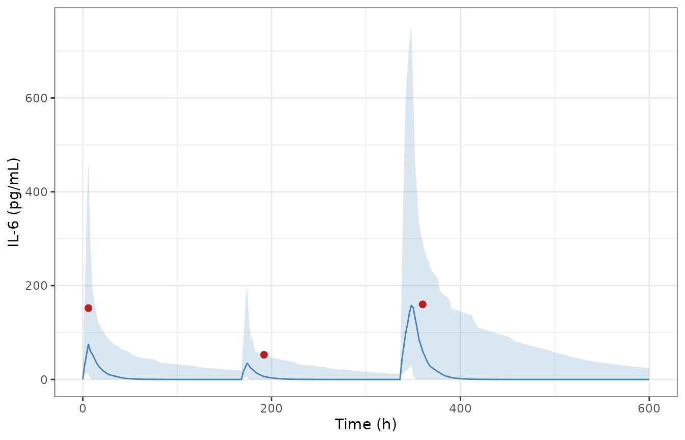
Simulated IL-6 median and 5th-95th percentile band over cycle 1, with observed mean peaks (red points). Compare Figure 3a of Chen 2024.
peak_band <- pop |>
  filter(time >= 336) |>
  group_by(id) |>
  summarise(peak = max(Cc), .groups = "drop")

data.frame(
  Statistic = c("5th percentile", "Median", "95th percentile"),
  `Simulated C1D15 peak (pg/mL)` = round(
    quantile(peak_band$peak, c(0.05, 0.5, 0.95)), 1
  ),
  `Observed C1D15 (pg/mL)` = c(1.57, 160, 910),
  check.names = FALSE,
  row.names = NULL
) |>
knitr::kable()| Statistic | Simulated C1D15 peak (pg/mL) | Observed C1D15 (pg/mL) |
|---|---|---|
| 5th percentile | 29.4 | 1.57 |
| Median | 162.1 | 160.00 |
| 95th percentile | 757.8 | 910.00 |
The median tracks the observed C1D15 mean closely (about 162 vs 160 pg/mL), and the upper percentile is within reach of the observed 910 pg/mL, which is what the inflated CVs were chosen to achieve.
The lower percentile is a different matter, and it is not a model deficiency. The observed 5th-percentile peak is reported as 1.57 pg/mL “for all days” – identical across three doses, which is the signature of a censored value rather than a measurement. Appendix S1 gives the ELISA’s validated range as 3.13 to 300 pg/mL, and 1.57 is exactly half of 3.13: the observed 5th percentile is the standard below-limit-of-quantification imputation at LLOQ/2. A model with no assay floor cannot reproduce it, and should not be expected to. Note also that the observed 95th percentile of 910 pg/mL sits well above the assay’s validated upper limit of 300 pg/mL, so it depends on dilution beyond the validated range.
Assumptions and deviations
Scope.
- The midazolam and simvastatin DDI layer is not
implemented. Those simulations used unmodified proprietary Simcyp V17
compound files whose in vivo clearances cannot be reconstructed from
Tables S1 and S2 (
Vmax/Kmare given per pmol of isoform, and MPPGL, liver weight, hepatic blood flow, andQgutare not reported). Tables 2, 3, S3, and S4 of the paper are therefore not reproducible here. - Mosunetuzumab pharmacokinetics are not modelled, because the paper does not model them. IL-6 enters as hypothetical infusions hand-calibrated to the observed profile.
Structural deviations.
-
Minimal PBPK reduced to one compartment. The
published Layer A is Simcyp’s minimal PBPK model with a single adjusting
compartment (SAC). Table 1 reports
Vsac0.05 L/kg but alsokin/kout= 0 (“Default (not used)”), so the SAC is kinetically disconnected and exchanges nothing; it acts only as bookkeeping that shrinks the effective systemic volume through the Table 1 footnote relationVsys = Vss - Vliver - Vsac. NeitherVlivernor the hepatic blood flow is reported, soVsyscannot be computed andVss= 0.43 L/kg is used directly as the one-compartment volume. -
Layer A does not reproduce the observed IL-6 peaks.
With the published
CL= 2.8 L/h andVss= 0.43 L/kg, the reduced model gives C1D1 and C1D8 peaks about 1.5-fold below the observed means, and a C1D15 peak above the observed mean. The C1D15 direction is consistent with the paper’s own remark that “the simulated mean IL-6 peak level in C1D15 is substantially higher than the observed peak levels in C1D1 and C1D8” – the authors deliberately over-drove C1D15 so the simulated 95th percentile would cover the highest observed values. The C1D1 under-prediction is a genuine gap attributable to the un-recoverable minimal-PBPK topology. No parameter was adjusted to close it. The enzyme layer is validated against IL-6 concentration directly (Checks 3 and 4), so this gap does not contaminate the Layer B validation. -
Table 1’s RA infusion amounts are not self-consistent with
CL= 2.8 L/h. Footnote d states that 0.0484 and 0.0968 mg infused over 21 days achieve steady-state IL-6 of 50 and 100 pg/mL. Under the reduced model those amounts give 34.3 and 68.6 pg/mL. The two amounts are in exact 2:1 ratio, matching the 2:1 target ratio, so the discrepancy is a calibration offset in the absolute clearance rather than an error in the amounts. Check 3 therefore clamps IL-6 to the stated concentrations (50 and 100 pg/mL), which is how Figure 4c is described in the paper, rather than using the stated amounts. -
Gut suppression is driven by systemic IL-6. The
paper states that the degree of gut CYP3A suppression is assumed similar
to that in the liver when the gut effect is considered, so both tissues
see the same driving concentration and differ only through
kdeg. - Healthy-volunteer baseline abundances are used. Table 1 footnote f states the rheumatoid-arthritis abundances were reset to healthy-volunteer levels whenever CYP3A suppression was predicted from in vitro data, and Figure 4c reports reduction from the healthy-volunteer baseline. The RA values (82.2 and 40.0) are used as validation targets in Check 3 rather than as inputs. Both baselines cancel out of the relative-activity outputs.
Unreported quantities.
-
No residual error is reported. The source is a
simulation exercise, not a fitted population model, so
propSdis fixed at 0 rather than invented. -
Between-subject variability is scenario-dependent.
Table 1 gives 200 %CV (CLint) and 100 %CV (Vss) for the mosunetuzumab
application but 30 %CV for both in the verification runs. The
application values are encoded, since that is the paper’s headline
analysis; substitute
omegaoflog(1 + 0.30^2)= 0.0862 to reproduce the verification setting. The CV on clearance is reported againstCLintrather thanCL;CLis a monotone function ofCLint, so the CV carries across.
Errata and internal inconsistencies in the source.
- Table 1 footnote c gives the hypothetical infusion timing as “6, 6, 13 h on days 1, 9, and 15” while the dosing regimen everywhere else is C1D1 / C1D8 / C1D15. Day 9 is most likely a typo for day 8, though note the observed C1D8 peak is recorded “on C1D9, 24 h postdose”, so the two may be conflated. Day 8 is used here.
-
Eminis described in Table 1 as “the minimum CYP3A enzyme activity (21.7%)” but entered in Simcyp asIndmax= 0.217, i.e. a fold multiplier. Reading it as “21.7% suppression” instead of “suppressed to 21.7% of control” inverts the effect size. The fold-multiplier reading is the one that reproduces Figure 4c, and is the one used here. - Table 1 gives the RA CYP3A4 abundance as “82.2/40.0” with a single slash where the healthy-volunteer row uses a double slash (“137//66.2”) for the liver//gut separator.
- Table 2’s Note and Methods disagree on the hip-surgery discharge window: the Note says “3-6 days, mean 4 days”, Methods says “days 2-6, mean 4 days”.
- The observed IL-6 peak at C1D8 is reported at 24 h post-dose, but
the hypothetical IL-6 infusion for that dose lasts only 6 h, so the
reduced model peaks at 6 h. The
tmaxrows of the NCA comparison reflect this; it is a property of the paper’s hand-calibrated infusion device, not of the enzyme model. - The reported 5th-percentile observed IL-6 peak of 1.57 pg/mL is identical across all three cycle-1 doses and is exactly half the assay’s validated lower limit of 3.13 pg/mL (Appendix S1) – i.e. a below-limit-of-quantification value imputed at LLOQ/2, not an observed concentration. The reported 95th percentile of 910 pg/mL likewise exceeds the assay’s validated upper limit of 300 pg/mL. Neither is treated here as a target the model should reproduce.
Session info
sessionInfo()
#> R version 4.6.1 (2026-06-24)
#> Platform: x86_64-pc-linux-gnu
#> Running under: Ubuntu 24.04.5 LTS
#>
#> Matrix products: default
#> BLAS:   /usr/lib/x86_64-linux-gnu/openblas-pthread/libblas.so.3
#> LAPACK: /usr/lib/x86_64-linux-gnu/openblas-pthread/libopenblasp-r0.3.26.so;  LAPACK version 3.12.0
#>
#> locale:
#>  [1] LC_CTYPE=C.UTF-8       LC_NUMERIC=C           LC_TIME=C.UTF-8
#>  [4] LC_COLLATE=C.UTF-8     LC_MONETARY=C.UTF-8    LC_MESSAGES=C.UTF-8
#>  [7] LC_PAPER=C.UTF-8       LC_NAME=C              LC_ADDRESS=C
#> [10] LC_TELEPHONE=C         LC_MEASUREMENT=C.UTF-8 LC_IDENTIFICATION=C
#>
#> time zone: UTC
#> tzcode source: system (glibc)
#>
#> attached base packages:
#> [1] stats     graphics  grDevices utils     datasets  methods   base
#>
#> other attached packages:
#> [1] ggplot2_4.0.3         dplyr_1.2.1           PKNCA_0.12.1
#> [4] rxode2_5.1.8          nlmixr2lib_0.3.2.9000
#>
#> loaded via a namespace (and not attached):
#>  [1] gtable_0.3.6        xfun_0.61           bslib_0.12.0
#>  [4] rxode2lincmt_0.1.0  lattice_0.22-9      vctrs_0.7.3
#>  [7] tools_4.6.1         generics_0.1.4      parallel_4.6.1
#> [10] tibble_3.3.1        symengine_0.2.14    pkgconfig_2.0.3
#> [13] data.table_1.18.6.1 checkmate_2.3.4     RColorBrewer_1.1-3
#> [16] S7_0.2.2            desc_1.4.3          lifecycle_1.0.5
#> [19] compiler_4.6.1      farver_2.1.2        textshaping_1.0.5
#> [22] fontawesome_0.5.3   htmltools_0.5.9     sys_3.4.3
#> [25] sass_0.4.10         yaml_2.3.12         tidyr_1.3.2
#> [28] pillar_1.11.1       pkgdown_2.2.1       crayon_1.5.3
#> [31] jquerylib_0.1.4     whisker_0.4.1       openssl_2.4.2
#> [34] cachem_1.1.0        nlme_3.1-169        tidyselect_1.2.1
#> [37] digest_0.6.39       lotri_1.0.5         purrr_1.2.2
#> [40] labeling_0.4.3      rxode2ll_2.0.18     fastmap_1.2.0
#> [43] grid_4.6.1          cli_3.6.6           dparser_1.3.1-14
#> [46] magrittr_2.0.5      withr_3.0.3         scales_1.4.0
#> [49] backports_1.5.1     rmarkdown_2.32      otel_0.2.0
#> [52] askpass_1.2.1       ragg_1.5.2          memoise_2.0.1
#> [55] evaluate_1.0.5      knitr_1.52          rex_1.2.2
#> [58] PreciseSums_0.7     rlang_1.3.0         downlit_0.4.5
#> [61] Rcpp_1.1.2          glue_1.8.1          xml2_1.6.0
#> [64] jsonlite_2.0.0      R6_2.6.1            systemfonts_1.3.2
#> [67] fs_2.1.0