Breakthrough bleeding on combined oral contraceptives (Chen 2024)
Source:vignettes/articles/Chen_2024_combinedOralContraceptives_btb.Rmd
Chen_2024_combinedOralContraceptives_btb.RmdModel and source
- Citation: Chen H, Chun D, Lingineni K, Guzy S, Cristofoletti R, Hoechel J, Jiao T, Cicali B, Vozmediano V, Schmidt S. Development of breakthrough bleeding model of combined-oral contraceptives utilizing model-based meta-analysis. CPT Pharmacometrics Syst Pharmacol. 2024;13(11):2016-2025. doi:10.1002/psp4.13261.
- Article: https://doi.org/10.1002/psp4.13261 (Open Access; PMC11578130)
- Supplement (Data S1-S5): Table S1 search criteria, Table S2 the full 33-arm analysis dataset with imputed covariates, Table S3 simulated BTB at months 1 / 3 / 4, Table S4 time to return to baseline, Figure S1 goodness-of-fit plots. Tables S3 and S4 are the validation targets used below.
- Errata: none. Crossref
update-toandupdated-byare both null; a PubMed / Google Scholar search for a correction notice returned nothing.
Breakthrough bleeding (BTB) – unscheduled bleeding during active hormone intake – is the most common reason women discontinue a combined oral contraceptive (COC). Chen 2024 pooled 228 aggregate BTB observations from 33 treatment arms of 25 published trials to establish the dose-response of BTB against the ethinyl estradiol (EE) and progestin components of a COC.
Why this is an extraction and not a systematic-review skip
The Methods describe a systematic literature search (PubMed, Cochrane, EMBASE, run with Excelra Knowledge Solutions) that returned 1147 papers, so the usual exclusion of systematic reviews applies to the data collection step only. The model itself is original: the authors fit it in NONMEM 7.5.0 with FOCEI, report their own structural-model selection (mono- vs bi- vs tri-exponential), their own stepwise covariate analysis, their own bootstrap (1000 resamples), and their own VPC. Table 2 is their parameter table, not a catalogue of other authors’ models.
Population
| Field | Value |
|---|---|
| Species | human |
| Disease state | healthy women using a combined oral contraceptive for pregnancy prevention. Alternative COC indications were an exclusion criterion. |
| Studies / arms / observations | 25 / 33 / 228 |
| Enrolled women (sum of Table S2 arm sizes) | 112,188 |
| Arm-mean age | treatment-arm mean age 16.4-40.2 years (Chen 2024 Table 1 total row and Table S2); the 16.4-year arm is an adolescent cohort. Individual ages are not available - this is aggregate published data. |
| Arm-mean body weight | treatment-arm mean body weight 46.0-68.3 kg (Table S2) |
| Regimens | conventional 21/7 monophasic COC regimens: ethinyl estradiol 15, 20, 30 or 35 ug/day combined with desogestrel 150 ug, drospirenone 3000 ug, gestodene 60 or 75 ug, or levonorgestrel 100 or 150 ug per day (Chen 2024 Table 1, Table S2). |
This is aggregate published data: the observation unit is a treatment arm, not a woman, and the model’s random effects are inter-study variance (ISV), not between-subject variance. Arm sizes span 30 to 95,906 women, and the enrolment total above is dominated by a single very large arm (Brill et al., n = 95,906), so it should be read as an enrolment count rather than an effective sample size.
The full population metadata, including the analysis-set construction
and the covariate-imputation scheme, is available programmatically via
readModelDb("Chen_2024_combinedOralContraceptives_btb_mbma")()$population.
Model structure
The final model (Chen 2024 Equation 3) is a bi-exponential decline in the fraction of women in an arm reporting BTB:
with a rapid initial phase (, ) and a slow second phase (, ). A one-exponential form gave biased estimates at later times and a three-exponential form was unstable and did not improve the fit (Results).
Two covariates are retained (Equations 4-7), both as power terms on a normalized covariate:
while and carry ISV only. The EE exponent is negative, so lower EE doses raise the slow-phase intercept and lengthen the time BTB takes to subside – the paper’s central finding. Progestin type is not a separate covariate: the four progestins are distinguished purely by their molar dose, which is why the analysis used molar rather than mass doses.
The time origin
Chen 2024 set “the time of the first observation … to 0,
corresponding to the completion of one full cycle of COC treatment”. So
the model’s time axis is
and a published “month
of COC treatment” value is read at time = M - 1. Every
comparison below applies that offset explicitly. Getting it wrong shifts
the whole trajectory by one month, which for the fast phase
(/month)
is more than a two-fold error in BTB.
Source trace
Every ini() entry carries an in-file comment naming its
source location in
inst/modeldb/therapeuticArea/Chen_2024_combinedOralContraceptives_btb_mbma.R.
The table collects them for review; the values shown are read out of the
packaged model, so this table cannot drift from the file.
| Quantity | Model value | Paper value | Source |
|---|---|---|---|
| A (initial-phase intercept) | 0.0383 | 0.0383 | Table 2, fixed effects |
| alpha (initial decline, 1/mo) | 0.9220 | 0.922 | Table 2, fixed effects |
| B (second-phase intercept) | 0.0134 | 0.0134 | Table 2, fixed effects |
| beta (slow decline, 1/mo) | 0.0524 | 0.0524 | Table 2, fixed effects |
| EE-dose exponent on B | -2.4500 | -2.45 | Table 2, ‘EE dose on B’ |
| Progestin-dose exponent on alpha | 0.5760 | 0.576 | Table 2, ‘Progestin dose by MW on alpha’ |
| ISV-A (log-scale variance) | 0.8240 | 0.824 | Table 2, random effects |
| ISV-alpha (log-scale variance) | 0.9590 | 0.959 | Table 2, random effects |
| ISV-B (log-scale variance) | 0.2230 | 0.223 | Table 2, random effects |
| ISV-beta (log-scale variance) | 0.1380 | 0.138 | Table 2, random effects |
| Unit-arm residual SD | 0.2025 | sqrt(0.0410) = 0.2025 | Table 2, RUV |
Structural equations: Equation 3 (bi-exponential), Equations 4-7 (the log-scale individual-parameter models), Equation 8 (additive residual on the BTB fraction) and Equation 9 (the arm-size-weighted residual variance).
Regimens simulated
Chen 2024 simulated nine FDA-approved progestin/EE combinations (Methods, and Tables S3 / S4). Molar progestin doses are obtained by dividing the mass dose by the progestin molecular weight.
mw <- c(DSG = 310.48, DRSP = 366.50, GSD = 310.43, LNG = 312.45)

regimens <- tibble::tribble(
  ~progestin, ~prog_ug, ~ee_ug,
  "GSD",         60,      15,
  "DRSP",      3000,      20,
  "DSG",        150,      20,
  "GSD",         75,      20,
  "LNG",        100,      20,
  "DRSP",      3000,      30,
  "DSG",        150,      30,
  "GSD",         75,      30,
  "LNG",        150,      30
) |>
  dplyr::mutate(
    prog_umol = unname(prog_ug / mw[progestin]),
    regimen   = sprintf("%s %g/%g", progestin, prog_ug, ee_ug)
  )

# The 0.48 umol normalization constant in Equation 5 is not named in the text.
# It is exactly the levonorgestrel 150 ug molar dose, which is what pins the
# molecular-weight convention above: no other MW set reproduces 0.48 for the
# paper's reference regimen.
stopifnot(abs(150 / mw[["LNG"]] - 0.48) < 0.005)

regimens |>
  dplyr::mutate(prog_umol = round(prog_umol, 3)) |>
  dplyr::select(-regimen) |>
  dplyr::rename("Progestin" = progestin, "Progestin dose (ug)" = prog_ug,
                "EE dose (ug)" = ee_ug, "Progestin dose (umol)" = prog_umol) |>
knitr::kable(caption = "The nine approved regimens Chen 2024 simulated.")| Progestin | Progestin dose (ug) | EE dose (ug) | Progestin dose (umol) |
|---|---|---|---|
| GSD | 60 | 15 | 0.193 |
| DRSP | 3000 | 20 | 8.186 |
| DSG | 150 | 20 | 0.483 |
| GSD | 75 | 20 | 0.242 |
| LNG | 100 | 20 | 0.320 |
| DRSP | 3000 | 30 | 8.186 |
| DSG | 150 | 30 | 0.483 |
| GSD | 75 | 30 | 0.242 |
| LNG | 150 | 30 | 0.480 |
Check 1 – the typical-value trajectory matches the closed form exactly
The most direct structural gate: solve the packaged model with the random effects zeroed, and compare against Equation 3 evaluated from the literals transcribed out of Table 2. Both covariate power terms are exercised. A mistyped estimate, an inverted exponent sign, or a covariate normalized to the wrong reference all fail here.
grid_t <- seq(0, 36, by = 1)

typ_events <- regimens |>
  dplyr::mutate(id = dplyr::row_number()) |>
  tidyr::expand_grid(time = grid_t) |>
  dplyr::transmute(
    id, time, evid = 0L,
    DOSE_EE_UG = ee_ug, DOSE_PROGESTIN_UMOL = prog_umol, regimen
  )

sim_typ <- rxode2::rxSolve(
  rxode2::zeroRe(ui), events = typ_events, keep = "regimen"
) |>
  as.data.frame() |>
  dplyr::mutate(regimen = as.character(regimen))
#> ℹ omega/sigma items treated as zero: 'eta_isv_a', 'eta_isv_alpha', 'eta_isv_b', 'eta_isv_beta'
#> Warning: multi-subject simulation without without 'omega'

# Equation 3 rebuilt from Table 2 literals -- deliberately NOT from the model's
# emitted a_btb / alpha_btb / b_btb / beta_btb, so the two sides are independent.
closed_form <- function(t, prog_umol, ee_ug) {
  0.0383 * exp(-0.922 * (prog_umol / 0.48)^0.576 * t) +
    0.0134 * (ee_ug / 30)^(-2.45) * exp(-0.0524 * t)
}

chk1 <- sim_typ |>
  dplyr::left_join(regimens |> dplyr::select(regimen, prog_umol, ee_ug),
                   by = "regimen") |>
  dplyr::mutate(
    expected = closed_form(time, prog_umol, ee_ug),
    rel_diff = abs(Cc - expected) / expected
  )

max(chk1$rel_diff)
#> [1] 2.147433e-15

# Same drawn (here: zeroed) parameters on both sides, so the difference is pure
# floating-point noise and a tight bound is the correct assertion.
stopifnot(max(chk1$rel_diff) < 1e-8)
Check 2 – the covariate power terms
Both covariates enter as . The alternative reading of Equations 5 and 6 – inside the logarithm, i.e. – is arithmetically impossible: with it makes negative at every EE dose, and it would put the typical at rather than the 0.922 Table 2 reports at the reference dose. The ratios below confirm the power form is what the model encodes.
at0 <- sim_typ |>
  dplyr::filter(time == 0) |>
  dplyr::left_join(regimens |> dplyr::select(regimen, prog_umol, ee_ug),
                   by = "regimen")

# B is the only EE-dependent term, and at t = 0 the model gives A + B, so B is
# recovered by subtracting the (EE-independent) A.
A_typ <- 0.0383
B_of <- function(rg) at0$Cc[at0$regimen == rg] - A_typ

b_ratio_20 <- B_of("LNG 100/20") / B_of("LNG 150/30")
b_ratio_15 <- B_of("GSD 60/15")  / B_of("LNG 150/30")

c(`B(20 ug)/B(30 ug)` = b_ratio_20, `B(15 ug)/B(30 ug)` = b_ratio_15)
#> B(20 ug)/B(30 ug) B(15 ug)/B(30 ug)
#>          2.700372          5.464161

stopifnot(
  isTRUE(all.equal(b_ratio_20, (20 / 30)^(-2.45), tolerance = 1e-6)),
  isTRUE(all.equal(b_ratio_15, (15 / 30)^(-2.45), tolerance = 1e-6))
)

# alpha appears only in the fast exponential. Recover it from the model's own
# emitted alpha_btb column and check the progestin-dose power term against the
# literal exponent. DRSP 3000 ug = 8.19 umol is 17-fold the 0.48 umol
# reference, so its fast phase should be about 5-fold faster.
alpha_drsp <- at0$alpha_btb[at0$regimen == "DRSP 3000/30"]
alpha_lng  <- at0$alpha_btb[at0$regimen == "LNG 150/30"]
drsp_umol  <- regimens$prog_umol[regimens$regimen == "DRSP 3000/30"]
lng_umol   <- regimens$prog_umol[regimens$regimen == "LNG 150/30"]

stopifnot(
  # LNG 150 ug is 0.480077 umol, not exactly the paper's rounded 0.48 umol
  # reference, so alpha there is the typical value scaled by
  # (0.480077/0.48)^0.576 -- a 0.009% correction, but assert it exactly rather
  # than loosening the tolerance until 0.922 fits.
  isTRUE(all.equal(alpha_lng, 0.922 * (lng_umol / 0.48)^0.576,
                   tolerance = 1e-9)),
  # The ratio cancels theta_alpha and the reference, isolating the power term.
  isTRUE(all.equal(alpha_drsp / alpha_lng,
                   (drsp_umol / lng_umol)^0.576, tolerance = 1e-9))
)
round(c(alpha_LNG = alpha_lng, alpha_DRSP = alpha_drsp,
        ratio = alpha_drsp / alpha_lng), 3)
#>  alpha_LNG alpha_DRSP      ratio
#>      0.922      4.723      5.122
Check 3 – the ISV terms are variances, not standard deviations
Table 2 prints each ISV alongside a percent-CV. For a log-normal random effect , so the printed CVs are only recovered if the tabulated numbers are variances on the log scale. This is the classic MBMA transcription trap and it is worth a dedicated gate: reading 0.824 as an SD would understate the spread of across studies by a wide margin.
isv <- tibble::tribble(
  ~term,       ~name,             ~published_cv,
  "ISV-A",     "eta_isv_a",       113.0,
  "ISV-alpha", "eta_isv_alpha",   127.0,
  "ISV-B",     "eta_isv_b",        49.9,
  "ISV-beta",  "eta_isv_beta",     38.5
) |>
  dplyr::mutate(
    variance   = vapply(name, getpar, numeric(1)),
    cv_as_var  = 100 * sqrt(exp(variance) - 1),
    cv_as_sd   = 100 * sqrt(exp(variance^2) - 1)
  )

isv |>
  dplyr::mutate(dplyr::across(c(cv_as_var, cv_as_sd), \(x) round(x, 1))) |>
  dplyr::select(-name) |>
  dplyr::rename("Term" = term, "Encoded value" = variance,
                "Published %CV" = published_cv,
                "%CV if variance" = cv_as_var, "%CV if SD" = cv_as_sd) |>
knitr::kable(caption = "Reading the ISV terms as log-scale variances recovers Table 2's printed CVs.")| Term | Published %CV | Encoded value | %CV if variance | %CV if SD |
|---|---|---|---|---|
| ISV-A | 113.0 | 0.824 | 113.1 | 98.6 |
| ISV-alpha | 127.0 | 0.959 | 126.8 | 122.8 |
| ISV-B | 49.9 | 0.223 | 50.0 | 22.6 |
| ISV-beta | 38.5 | 0.138 | 38.5 | 13.9 |
# Table 2 prints the CVs to 3 significant figures, so 0.6 percentage points is
# ample rounding headroom on the largest (113%) term.
stopifnot(all(abs(isv$cv_as_var - isv$published_cv) < 0.6))

# The discriminating counterfactual, summed over the four terms so no single
# term has to carry it: reading the same numbers as SDs mis-states the CVs by
# tens of percentage points in total. (Per-term it misses by 14.4, 4.2, 27.3
# and 24.6 points -- the alpha term alone is not decisive, which is exactly why
# the gate is on the sum.)
stopifnot(
  sum(abs(isv$cv_as_var - isv$published_cv)) <  1.5,
  sum(abs(isv$cv_as_sd  - isv$published_cv)) > 20
)
Check 4 – the residual error and its arm-size weighting
Chen 2024 Equation 9 gives , where is the number of women in the arm. Table 2 reports labelled “(20.2% CV)”, and , which confirms 0.0410 is the variance.
nlmixr2’s add() takes a single population
parameter and cannot read a per-record arm size, so addSd
encodes the unit-arm SD
.
The SD actually applying to an arm of
women is addSd / sqrt(N).
add_sd <- getpar("addSd")
stopifnot(isTRUE(all.equal(add_sd^2, 0.0410, tolerance = 1e-3)))

# Median arm in this analysis is 308 women (Table 1 total row).
data.frame(
  `Arm size (N)` = c(30, 308, 5602, 95906),
  `Residual SD (BTB fraction)` = round(add_sd / sqrt(c(30, 308, 5602, 95906)), 5),
  check.names = FALSE
) |>
knitr::kable(caption = "Arm-size-weighted residual SD, addSd / sqrt(N), across the observed range of arm sizes.")| Arm size (N) | Residual SD (BTB fraction) |
|---|---|
| 30 | 0.03697 |
| 308 | 0.01154 |
| 5602 | 0.00271 |
| 95906 | 0.00065 |
For the median 308-woman arm the residual SD is about 1.2 percentage points of BTB, which is the right order of magnitude next to the 4-12% BTB rates the model predicts. The very large arms are, correctly, weighted almost as exact observations.
Virtual cohort of study arms
The random effects are inter-study, so a “cohort” here is a set of simulated study arms, each drawing its own , , , . 200 arms per regimen (the per-arm cap) are simulated. Each regimen is re-seeded with the same seed so all nine share common random numbers – that makes the between-regimen contrasts, which is what Tables S3 and S4 report, far more precise than independent draws would at this cohort size.
n_arms <- 200L

sim_one <- function(i) {
  r <- regimens[i, ]
  # Re-seed inside the loop so every regimen draws the SAME etas (common random
  # numbers). rxSetSeed fixes rxode2's stream per solver thread, so the absolute
  # draw still differs across machines -- every assertion below is written to
  # hold for any cohort the model can produce.
  rxode2::rxSetSeed(20260906)
  ev <- tidyr::expand_grid(id = seq_len(n_arms), time = grid_t) |>
    dplyr::mutate(
      evid = 0L,
      DOSE_EE_UG = r$ee_ug, DOSE_PROGESTIN_UMOL = r$prog_umol
    )
  # The event table already carries `n_arms` distinct ids, so rxSolve draws one
  # eta vector per id from the model's omega; nSub would double-specify it.
  rxode2::rxSolve(ui, events = ev) |>
    as.data.frame() |>
    dplyr::mutate(regimen = r$regimen, id = id + (i - 1L) * n_arms)
}

sim <- dplyr::bind_rows(lapply(seq_len(nrow(regimens)), sim_one))

# IDs must be disjoint across regimens, or any later group-by silently merges
# arms from different regimens into one.
stopifnot(
  length(unique(sim$id)) == nrow(regimens) * n_arms,
  !anyDuplicated(sim[, c("id", "time")])
)
Replicate Figure 4 – BTB decline by regimen
baseline_btb <- 0.0168  # Methods 'Data': untreated unscheduled-bleeding rate.

sim |>
  dplyr::group_by(regimen, time) |>
  dplyr::summarise(
    Q10 = quantile(Cc, 0.10), Q50 = median(Cc), Q90 = quantile(Cc, 0.90),
    .groups = "drop"
  ) |>
  dplyr::left_join(regimens |> dplyr::select(regimen, ee_ug), by = "regimen") |>
  dplyr::mutate(
    month  = time + 1,                      # months since COC initiation
    ee_lab = paste0("EE ", ee_ug, " ug")
  ) |>
  ggplot(aes(month, 100 * Q50, colour = regimen, fill = regimen)) +
  geom_ribbon(aes(ymin = 100 * Q10, ymax = 100 * Q90), alpha = 0.12,
              colour = NA) +
  geom_line(linewidth = 0.8) +
  geom_hline(yintercept = 100 * baseline_btb, linetype = "dashed",
             colour = "red") +
  facet_wrap(~ee_lab) +
  coord_cartesian(xlim = c(1, 25), ylim = c(0, 30)) +
  labs(
    x = "Months since COC initiation", y = "Women experiencing BTB (%)",
    title = "BTB decline after COC initiation, by progestin/EE regimen",
    caption = paste("Replicates Figure 4 of Chen 2024. Bands are the 10th-90th",
                    "percentiles across 200 simulated study arms. The red",
                    "dashed line is the 1.68% untreated baseline.")
  ) +
  theme(legend.position = "bottom")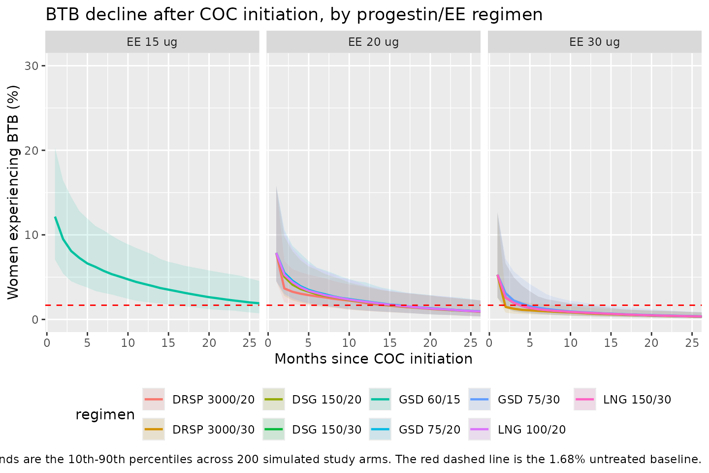
The EE dose, not the progestin, dominates: the three EE-15/20 panels sit well above the EE-30 panel throughout, and only the EE-30 regimens approach the untreated baseline within a few months.
Check 5 – simulated BTB against Table S3
Table S3 reports median BTB after 1, 3 and 4 months of COC treatment.
Applying the time origin, those are time = 0, 2 and 3.
published_s3 <- tibble::tribble(
  ~regimen,        ~m1,  ~m3,  ~m4,
  "GSD 60/15",    11.9,  8.2,  7.4,
  "DRSP 3000/20",  6.5,  3.4,  3.2,
  "DSG 150/20",    7.8,  4.3,  3.7,
  "GSD 75/20",     7.8,  4.7,  4.1,
  "LNG 100/20",    7.7,  4.4,  3.8,
  "DRSP 3000/30",  4.0,  1.3,  1.2,
  "DSG 150/30",    5.0,  1.9,  1.5,
  "GSD 75/30",     5.2,  2.4,  1.9,
  "LNG 150/30",    4.9,  1.9,  1.6
)

sim_s3 <- sim |>
  dplyr::filter(time %in% c(0, 2, 3)) |>
  dplyr::group_by(regimen, time) |>
  dplyr::summarise(sim_pct = 100 * median(Cc), .groups = "drop") |>
  dplyr::mutate(month = as.integer(time) + 1L)

cmp_s3 <- published_s3 |>
  tidyr::pivot_longer(c(m1, m3, m4), names_to = "month",
                      values_to = "published_pct") |>
  dplyr::mutate(month = as.integer(sub("^m", "", month))) |>
  dplyr::left_join(sim_s3, by = c("regimen", "month")) |>
  dplyr::mutate(pct_diff = 100 * (sim_pct - published_pct) / published_pct)

cmp_s3 |>
  dplyr::mutate(dplyr::across(c(sim_pct, published_pct, pct_diff),
                              \(x) round(x, 1))) |>
  dplyr::select(regimen, month, published_pct, sim_pct, pct_diff) |>
  dplyr::rename("Regimen" = regimen, "Month" = month,
                "Table S3 median BTB (%)" = published_pct,
                "Simulated median BTB (%)" = sim_pct,
                "Difference (%)" = pct_diff) |>
knitr::kable(caption = "Simulated vs Chen 2024 Table S3 median BTB.")| Regimen | Month | Table S3 median BTB (%) | Simulated median BTB (%) | Difference (%) |
|---|---|---|---|---|
| GSD 60/15 | 1 | 11.9 | 12.9 | 8.3 |
| GSD 60/15 | 3 | 8.2 | 8.6 | 4.8 |
| GSD 60/15 | 4 | 7.4 | 7.7 | 3.4 |
| DRSP 3000/20 | 1 | 6.5 | 8.3 | 27.4 |
| DRSP 3000/20 | 3 | 3.4 | 3.4 | 1.2 |
| DRSP 3000/20 | 4 | 3.2 | 3.1 | -2.2 |
| DSG 150/20 | 1 | 7.8 | 8.3 | 6.2 |
| DSG 150/20 | 3 | 4.3 | 4.4 | 1.5 |
| DSG 150/20 | 4 | 3.7 | 3.7 | 0.8 |
| GSD 75/20 | 1 | 7.8 | 8.3 | 6.2 |
| GSD 75/20 | 3 | 4.7 | 4.8 | 1.7 |
| GSD 75/20 | 4 | 4.1 | 4.2 | 2.6 |
| LNG 100/20 | 1 | 7.7 | 8.3 | 7.5 |
| LNG 100/20 | 3 | 4.4 | 4.6 | 5.1 |
| LNG 100/20 | 4 | 3.8 | 4.0 | 6.1 |
| DRSP 3000/30 | 1 | 4.0 | 5.4 | 34.0 |
| DRSP 3000/30 | 3 | 1.3 | 1.4 | 4.3 |
| DRSP 3000/30 | 4 | 1.2 | 1.2 | -0.8 |
| DSG 150/30 | 1 | 5.0 | 5.4 | 7.2 |
| DSG 150/30 | 3 | 1.9 | 2.1 | 9.1 |
| DSG 150/30 | 4 | 1.5 | 1.7 | 10.9 |
| GSD 75/30 | 1 | 5.2 | 5.4 | 3.1 |
| GSD 75/30 | 3 | 2.4 | 2.5 | 4.7 |
| GSD 75/30 | 4 | 1.9 | 2.0 | 4.1 |
| LNG 150/30 | 1 | 4.9 | 5.4 | 9.4 |
| LNG 150/30 | 3 | 1.9 | 2.1 | 9.3 |
| LNG 150/30 | 4 | 1.6 | 1.7 | 4.0 |
Months 3 and 4 are gated. Month 1 is a known deviation and is
excluded from the gate – see the Errata: at
time = 0 Equation 3 reduces to
,
which contains no
and therefore cannot differentiate progestins at a fixed EE dose, yet
Table S3’s month-1 row does.
gate_s3 <- dplyr::filter(cmp_s3, month %in% c(3, 4))

summary_s3 <- c(
  median_abs_pct_diff = median(abs(gate_s3$pct_diff)),
  p90_abs_pct_diff    = unname(quantile(abs(gate_s3$pct_diff), 0.9))
)
round(summary_s3, 1)
#> median_abs_pct_diff    p90_abs_pct_diff
#>                 4.0                 9.2

# Bounds are calibrated to the Monte Carlo noise of a 200-arm cohort, measured
# over 60 independent seeds: the median |% diff| across the nine regimens ranged
# 1.5-9.6% and the 90th percentile reached 19.9% in the worst seed. The bounds
# below sit outside that range with headroom, and remain far tighter than any
# parameter transcription error would produce (a one-place slip in alpha or the
# EE exponent moves these by hundreds of percent). Do not tighten them back.
stopifnot(
  summary_s3[["median_abs_pct_diff"]] < 15,
  summary_s3[["p90_abs_pct_diff"]]    < 40
)
Check 6 – time to return to baseline against Table S4
Table S4 reports the time for BTB to fall back to the 1.68% untreated unscheduled-bleeding rate. Each simulated arm’s macro-constants are read out of the solved model and Equation 3 is inverted numerically; the published values are measured from COC initiation, so one month is added back.
arms <- sim |>
  dplyr::filter(time == 0) |>
  dplyr::select(id, regimen, a_btb, alpha_btb, b_btb, beta_btb)

# Equation 3, vectorised over arms.
btb_at <- function(x, A, al, B, be) A * exp(-al * x) + B * exp(-be * x)

# Vectorised bisection for BTB(x) = 0.0168. BTB is monotone decreasing in x, so
# bisection converges to the tolerance implied by the iteration count
# (600 / 2^60 months).
time_to_baseline <- function(A, al, B, be, target = baseline_btb,
                             hi = 600, iter = 60) {
  lo <- rep(0, length(A))
  up <- rep(hi, length(A))
  for (k in seq_len(iter)) {
    mid <- (lo + up) / 2
    above <- btb_at(mid, A, al, B, be) > target
    lo <- ifelse(above, mid, lo)
    up <- ifelse(above, up, mid)
  }
  out <- (lo + up) / 2
  out[btb_at(0,  A, al, B, be) <= target] <- 0
  out[btb_at(hi, A, al, B, be) >  target] <- NA_real_
  out
}

arms$ttb <- time_to_baseline(arms$a_btb, arms$alpha_btb,
                             arms$b_btb, arms$beta_btb)
stopifnot(!anyNA(arms$ttb))  # no arm should still be bleeding at 50 years

published_s4 <- tibble::tribble(
  ~regimen,        ~published_median,
  "GSD 60/15",     28.6,
  "DSG 150/20",    15.6,
  "DRSP 3000/20",  14.9,
  "GSD 75/20",     15.9,
  "LNG 100/20",    16.0,
  "DSG 150/30",     3.4,
  "DRSP 3000/30",   1.6,
  "GSD 75/30",      4.8,
  "LNG 150/30",     3.7
)

cmp_s4 <- arms |>
  dplyr::group_by(regimen) |>
  # +1 converts the model's "months since first observation" axis back to
  # "months since COC initiation", which is what Table S4 reports.
  dplyr::summarise(sim_median = median(ttb) + 1, .groups = "drop") |>
  dplyr::left_join(published_s4, by = "regimen") |>
  dplyr::mutate(pct_diff = 100 * (sim_median - published_median) /
                  published_median)

cmp_s4 |>
  dplyr::mutate(dplyr::across(c(sim_median, published_median, pct_diff),
                              \(x) round(x, 1))) |>
  dplyr::rename("Regimen" = regimen,
                "Simulated median (months)" = sim_median,
                "Table S4 median (months)" = published_median,
                "Difference (%)" = pct_diff) |>
knitr::kable(caption = "Time for BTB to return to the 1.68% untreated baseline, measured from COC initiation.")| Regimen | Simulated median (months) | Table S4 median (months) | Difference (%) |
|---|---|---|---|
| DRSP 3000/20 | 15.1 | 14.9 | 1.6 |
| DRSP 3000/30 | 1.8 | 1.6 | 9.8 |
| DSG 150/20 | 15.7 | 15.6 | 0.9 |
| DSG 150/30 | 3.9 | 3.4 | 15.2 |
| GSD 60/15 | 29.9 | 28.6 | 4.4 |
| GSD 75/20 | 16.6 | 15.9 | 4.5 |
| GSD 75/30 | 4.9 | 4.8 | 1.1 |
| LNG 100/20 | 16.3 | 16.0 | 2.1 |
| LNG 150/30 | 3.9 | 3.7 | 6.0 |
summary_s4 <- c(
  median_abs_pct_diff = median(abs(cmp_s4$pct_diff)),
  p90_abs_pct_diff    = unname(quantile(abs(cmp_s4$pct_diff), 0.9))
)
round(summary_s4, 1)
#> median_abs_pct_diff    p90_abs_pct_diff
#>                 4.4                10.9

# Same 60-seed calibration as Check 5: median |% diff| ranged 2.0-11.5% and the
# 90th percentile reached 24.1% in the worst seed. Bounds sit outside that.
stopifnot(
  summary_s4[["median_abs_pct_diff"]] < 18,
  summary_s4[["p90_abs_pct_diff"]]    < 45
)

# The paper's qualitative conclusions, which are what a user of this model will
# rely on, must also survive. These are absolute statements from the Results /
# Discussion, not bounds taken from a single run.
ttb_by <- setNames(cmp_s4$sim_median, cmp_s4$regimen)
stopifnot(
  # "BTB ... typically returns to baseline within 3-4 months" at EE 30 ug,
  # "except for GSD (4.8 months)".
  all(ttb_by[c("DSG 150/30", "DRSP 3000/30", "LNG 150/30")] < 6),
  ttb_by[["GSD 75/30"]] < 8,
  # "it can take much longer for COC drug products that contain 20 ug EE"
  all(ttb_by[c("DSG 150/20", "DRSP 3000/20", "GSD 75/20", "LNG 100/20")] > 8),
  # "Median recovery time was the longest ... for the GSD/EE 60/15 formulation."
  ttb_by[["GSD 60/15"]] > max(ttb_by[names(ttb_by) != "GSD 60/15"])
)
Why there is no PKNCA section
PKNCA computes Cmax / Tmax / AUC / half-life from a
concentration-time profile. This model has no PK: there is no
compartment, no dose event, and no concentration. Its dependent variable
is a dimensionless proportion of an aggregate study arm
experiencing an adverse event, and the paper reports no NCA parameters.
The equivalent-strength validation is the set of checks above: an exact
closed-form gate on the structural equation, exact gates on both
covariate power terms and on the variance scale of every random effect,
and reproduction of the paper’s own two simulation tables. This follows
the endogenous / mechanistic carve-out and matches the sibling MBMA
vignettes (Hanan_2026_peginterferon_alfa_hbsag_loss,
Goteti_2024_SLE_mbma).
Assumptions and deviations
Errata and internal inconsistencies in the source
-
Table S3 month-1 row is not reproducible from Equation
3. At
time = 0(one completed COC cycle = “month 1”) the model gives , in which does not appear, so at a fixed EE dose all four progestins must predict the same BTB. Table S3’s month-1 row instead reports progestin-specific values (at EE 30 ug: DRSP 4.0%, LNG 4.9%, DSG 5.0%, GSD 5.2%). No single evaluation time reproduces that row: scanningtimefrom 0 to 5 months in 0.25-month steps, the best achievable root-mean-square relative error across the nine regimens is 15%, attained attime = 0– against 2.3% and 2.9% for the month-3 and month-4 rows at their corresponding times. The month-1 row is therefore excluded from the gate in Check 5 and recorded here rather than accommodated by widening the bound. Months 3 and 4 and the whole of Table S4 reproduce, so the structural extraction is sound. - Table S4 prints the gestodene 15 ug EE arm as “GSD 65 mcg”. Table 1, Table S2 and the Results text all give 60 ug for that arm (the marketed GSD/EE 60/15 product). 60 ug is used here.
- Table S2 row for study 23 arm 1 lists a 3000 ug progestin dose against progestin type “LNG”. 3000 ug is the drospirenone dose; levonorgestrel is dosed at 100-150 ug throughout the rest of the dataset. This affects the analysis dataset listing only, not any parameter.
-
Table 1 labels its height row “Mean HT (m)” but
prints centimetre values (e.g. 166.20). The model file records
HTin cm.
Modelling assumptions
- ISV covariances are not published. The Methods state “Covariances among the inter-study variance (ISV) were also estimated”, but Table 2 reports only the four diagonal terms and no covariance or correlation matrix appears anywhere in the paper or supplement. The model encodes a diagonal omega. Checks 5 and 6 show that a diagonal omega still reproduces the paper’s own Table S3 (months 3, 4) and Table S4 simulation summaries, so the omission is empirically tolerable, but a user refitting this model should not assume the off-diagonals are truly zero.
-
The arm-size residual weighting is carried, not
applied. Equation 9’s
cannot be expressed in
nlmixr2’sadd()syntax, soaddSdis the unit-arm SD and a user simulating a specific arm must scale it by1/sqrt(N)(Check 4). The paper’s own Table S3 / S4 simulations propagate the fixed effects and the ISV only, which is what the checks above do. - Progestin molecular weights are not printed in the paper. The molar conversion uses the standard values (DSG 310.48, DRSP 366.50, GSD 310.43, LNG 312.45 g/mol). These are validated rather than assumed: they are what makes the paper’s own unnamed 0.48 umol normalization constant come out exactly equal to the levonorgestrel 150 ug dose, and they reproduce Tables S3 and S4.
-
Extrapolation limits. EE dose is observed only over
15-35 ug and the power term diverges as EE approaches zero;
progestin-only pills were explicitly excluded from model development and
are not represented by setting
DOSE_EE_UG = 0. Molar progestin dose is observed over 0.19-8.19 umol. - Scope. The model predicts the aggregate BTB fraction of a treatment arm, not an individual woman’s bleeding outcome. The random effects are between-study, so simulating 200 “subjects” simulates 200 hypothetical study arms.