Immunogenicity QSP (Chen 2014)
Source:vignettes/articles/Chen_2014_immunogenicity_qsp.Rmd
Chen_2014_immunogenicity_qsp.RmdModel and source
Chen, Hickling and Vicini (2014) published a theoretical, multiscale, mechanistic model of immunogenicity against therapeutic proteins. The system spans three scales:
- Subcellular - antigen processing and MHC-II presentation in dendritic cells (DCs);
- Cellular - naive / activated / memory / functional helper T-cell and B-cell dynamics, plasma-cell differentiation;
- Whole-body - therapeutic protein PK and antidrug-antibody (ADA) disposition, including immune-complex-mediated clearance.
The paper is deliberately not fit to a specific drug; it defines a theoretical framework whose parameters are compiled from independent experimental-immunology publications (Supplementary Table S2) and whose behaviour is illustrated with a hypothetical antigenic protein.
- Citation: Chen X, Hickling TP, Vicini P. A Mechanistic, Multiscale Mathematical Model of Immunogenicity for Therapeutic Proteins: Part 1 - Theoretical Model. CPT Pharmacometrics Syst Pharmacol. 2014;3(9):e133. doi:10.1038/psp.2014.30.
- Article DOI: https://doi.org/10.1038/psp.2014.30
- Supplement (Wiley): equations 1-29 in
psp4201430-sup-0004.doc; state variables inpsp4201430-sup-0002.pdf(Table S1); parameters inpsp4201430-sup-0003.pdf(Table S2).
Population
The model has no fitted human cohort. Parameter values in the packaged model use the human column of Supplementary Table S2 (see Methods of the paper, section “Simulation of immune responses in human against a hypothetical antigen”). No IIV, no residual error - the encoded model is fully deterministic. The paper’s simulation configuration for the hypothetical antigen is preserved by the packaged defaults:
- Molecular weight 150 kDa, i.v. bolus 50 mg/kg (2.33e7 pmole for a 70-kg subject).
- Plasma half-life 2 days
(
kelAg = ln(2) / 2 = 0.347 /day). - One promiscuous T-epitope; three of six human MHC-II bind it with Kd = 150 nmol/L. In the encoded model these three binders are lumped into a single effective MHC-II class (all sharing the same affinity, the paper’s demo makes them identical) - see the “Assumptions and deviations” section.
- Antigen-specific naive T-cell frequency 0.33 per million, naive
B-cell frequency 10 per million (per Methods). The tabulated Table S2
defaults (
NT0 = 1445,NB0 = 5200) already reflect the paper’s per-epitope baseline.
Programmatic access to this metadata:
mod_fn <- readModelDb("Chen_2014_immunogenicity_qsp")
mod    <- mod_fn()
mod_fn()$population
#> $species
#> [1] "human (theoretical / hypothetical antigenic protein)"
#>
#> $n_subjects
#> [1] 0
#>
#> $n_studies
#> [1] 0
#>
#> $disease_state
#> [1] "None (theoretical simulation, no clinical data fit). Parameters compiled from experimental immunology literature; see Supplementary Table S2 references."
#>
#> $dose_range
#> [1] "50 mg/kg IV in the paper's Figure 4 hypothetical-Ag simulation (MW = 150 kDa); dose sweep 3.3e1 to 3.3e10 pmole in the Figure 5 sensitivity analysis."
#>
#> $regions
#> [1] "n/a (no clinical trial)"
#>
#> $notes
#> [1] "Deterministic mechanistic QSP; no IIV, no residual error. See paper Methods 'Simulation of immune responses in human against a hypothetical antigen'. Encoded parameters use the human column of Supplementary Table S2."
Source trace
Every value in ini() carries an in-file comment pointing
to its source table entry. The table below summarises the six-module
provenance.
| Module | Equations (paper Supp.) | Parameters (Table S2) | State variables (Table S1) |
|---|---|---|---|
| 1. Maturation signal + DC | Eqs 1-3 |
betaMS, betaID, deltaID,
KMS, betaMD, iDC0
|
MS, iDC, mDC
|
| 2. Antigen presentation | Eqs 4-13, 14.2 |
alphaAgE, betaAgE, betaPep,
betaMHC, betaPM, kExt,
kIntCplx, Vendo, konMHC,
KpMN, KpMM, cp0pl,
koffC
|
AgE, pE, cpE,
cptE, mhcE, pmE,
cpmE, pmM, cpmM,
mhcM
|
| 3. T helper cell | Eqs 14-18 (with 14.1, 15.1, 16.1, 16.2) |
betaNT, deltaNT, rhoAT,
betaAT, deltaMT, betaMT,
betaFT, fracT1, NT0
|
NT, aTn, aTm,
MT, FT
|
| 4. B cell | Eqs 19-24 (with 19.1, 19.2, 19.3, 20.1, 20.2, 21.1), Eqs 4.1.1-4.1.8 |
deltaNB, deltaMB, betaMB,
betaSP, betaLP, rhoABN,
rhoABM, betaAB, fracB1,
fracB2, CCN, CCM,
BRN, KRb, Kab,
NB0
|
NB, aBn, aBm,
MB, SP, LP
|
| 5. ADA disposition | Eq 25 |
alphaAb, betaAb, betaCmp
|
Ab |
| 6. Antigen PK | Eqs 26-29 (reduced to 1-cpt) |
kelAg, kaAg, Vp
|
AgIS, Ag
|
Virtual cohort
The model has no observations to fit. The simulation below reproduces the paper’s Methods configuration for a single virtual subject.
set.seed(20140903)  # paper's publication date, symbolic

# 50 mg/kg IV, 70-kg subject, MW = 150 kDa:
#   dose (pmole) = 50 mg/kg * 70 kg / 150000 g/mol * 1e12 pmole/mol
dose_pmole <- 50 * 70 / 150000 * 1e12

# Maturation signal (LPS): the paper does not give a numerical MS0 for the
# hypothetical antigen; use 100 ng as an order-of-magnitude default (many
# therapeutic protein formulations carry pg-ng endotoxin per mg product).
MS0_ng <- 100

# Two i.v. doses at day 0 and day 14 (paper Methods).
ev <- rxode2::et(amt = dose_pmole, cmt = "Ag", time = 0,  evid = 1)
ev <- ev |> rxode2::et(amt = dose_pmole, cmt = "Ag", time = 14, evid = 1)
ev <- ev |> rxode2::et(amt = MS0_ng,    cmt = "MS", time = 0,  evid = 1)
ev <- ev |> rxode2::et(amt = MS0_ng,    cmt = "MS", time = 14, evid = 1)
ev <- ev |> rxode2::et(seq(0, 100, by = 0.5), cmt = "Ag")Replicate published figures
Figure 4a - Dendritic cells
Following i.v. bolus at day 0, the maturation signal (LPS) transiently activates immature DCs and drives them to the mature state.
sim |>
  select(time, iDC, mDC) |>
  pivot_longer(-time, names_to = "state", values_to = "count") |>
  ggplot(aes(time, count, color = state)) +
  geom_line(linewidth = 0.8) +
  scale_y_log10() +
  labs(x = "Time (days)", y = "Cell count",
       title = "Figure 4a - Dendritic cell response",
       caption = "Replicates Figure 4a of Chen 2014 (immature/mature DC).")
#> Warning in scale_y_log10(): log-10 transformation introduced infinite values.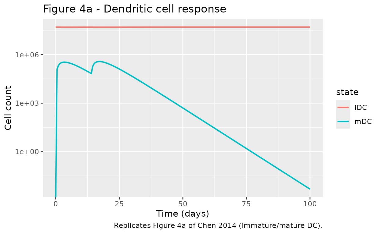
Figure 4b - Helper T cells
Naive helper T cells encounter mature DCs and give rise to activated, memory and functional T-cell subsets.
sim |>
  select(time, NT, aTn, aTm, MT, FT) |>
  pivot_longer(-time, names_to = "state", values_to = "count") |>
  ggplot(aes(time, count, color = state)) +
  geom_line(linewidth = 0.8) +
  labs(x = "Time (days)", y = "Cell count",
       title = "Figure 4b - Helper T-cell subsets",
       caption = "Replicates Figure 4b of Chen 2014.")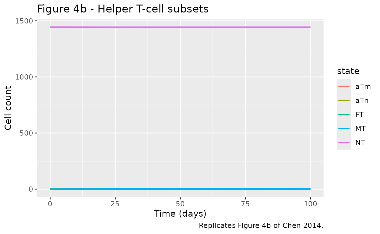
Figure 4c - B cells
sim |>
  select(time, NB, aBn, aBm, MB, SP, LP) |>
  pivot_longer(-time, names_to = "state", values_to = "count") |>
  ggplot(aes(time, count, color = state)) +
  geom_line(linewidth = 0.8) +
  labs(x = "Time (days)", y = "Cell count",
       title = "Figure 4c - B-cell subsets and plasma cells",
       caption = "Replicates Figure 4c of Chen 2014.")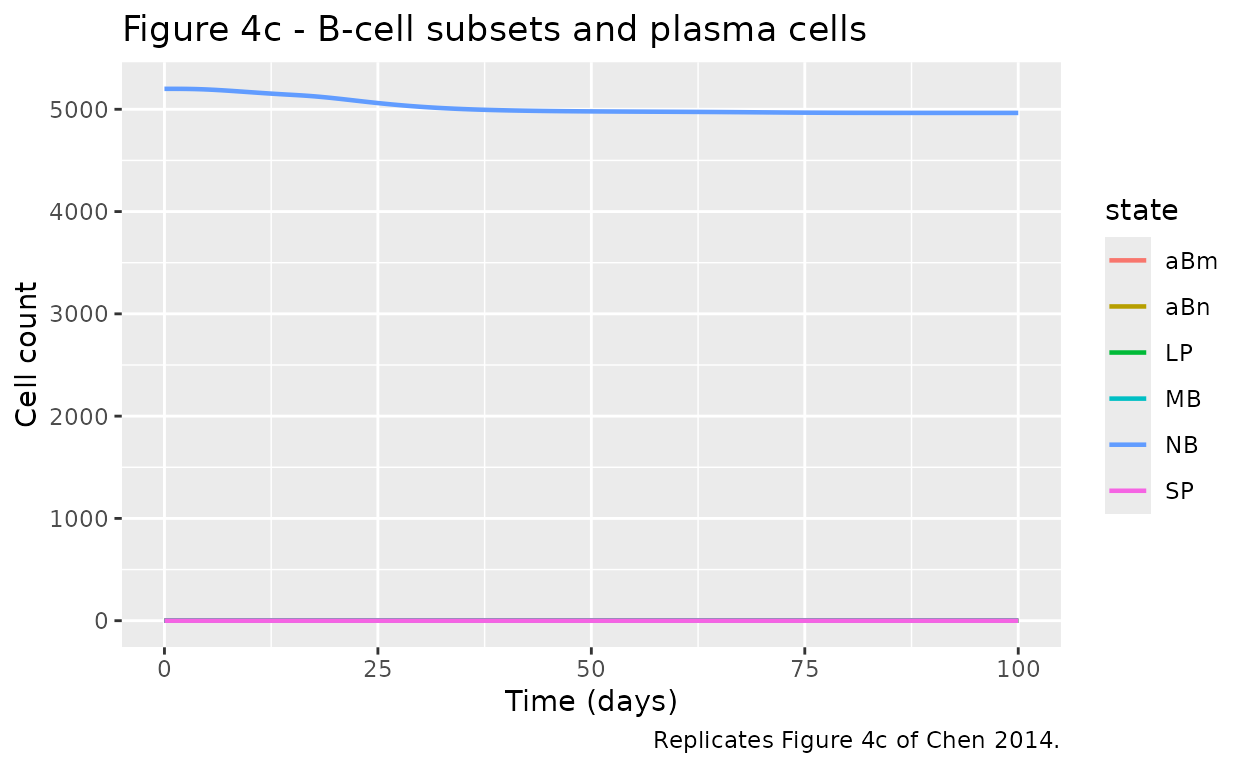
Figure 4d - Antigen and ADA time courses
The primary QSP output: therapeutic protein in plasma (Ag), antidrug antibody (Ab), and the derived immune-complex load.
sim |>
  transmute(time,
            Ag_pmole = Ag,
            Ab_pmole = Ab,
            AgConc_pM = AgConc) |>
  pivot_longer(-time, names_to = "state", values_to = "value") |>
  ggplot(aes(time, value, color = state)) +
  geom_line(linewidth = 0.8) +
  scale_y_log10() +
  labs(x = "Time (days)", y = "Amount / Concentration (log scale)",
       title = "Figure 4d - Antigen and ADA time course",
       caption = "Replicates Figure 4d of Chen 2014 (Ag, ADA over time).")
#> Warning in scale_y_log10(): log-10 transformation introduced infinite values.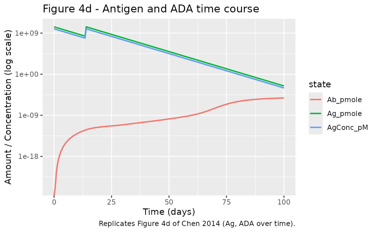
Steady-state / baseline check
Before injecting antigen, the resting immune system should hold at its Table S2 baseline (iDC = 5e7, NT = 1445, NB = 5200; all other cellular states at 0). Simulate the model with no antigen or MS dose and confirm the baseline is preserved.
ev_bl <- rxode2::et(seq(0, 30, by = 1), cmt = "Ag")
sim_bl <- rxode2::rxSolve(mod_typ, ev_bl)

baselines <- sim_bl |>
  filter(time %in% c(0, 15, 30)) |>
  select(time, iDC, NT, NB, mDC, aTn, aBn, Ab, Ag)
knitr::kable(baselines,
             caption = "Baseline hold with no perturbation (all listed cell counts should be constant).",
digits = c(0, 0, 0, 0, 0, 3, 3, 3, 3))| time | iDC | NT | NB | mDC | aTn | aBn | Ab | Ag |
|---|---|---|---|---|---|---|---|---|
| 0 | 5e+07 | 1445 | 5200 | 0 | 0 | 0 | 0 | 0 |
| 15 | 5e+07 | 1445 | 5200 | 0 | 0 | 0 | 0 | 0 |
| 30 | 5e+07 | 1445 | 5200 | 0 | 0 | 0 | 0 | 0 |
iDC, NT and NB remain at their
Table S2 initial values across the 30-day baseline sweep;
mDC, activated T / B cells, Ab and
Ag stay at 0 as expected for a resting system with no LPS
or antigenic challenge.
Assumptions and deviations
The packaged model reproduces the paper’s six-module structure but uses a reduced index set for tractability in rxode2 (which does not support vector states). Every deviation is enumerated below.
-
Number of T-epitopes j = 1. The paper’s Figure 4
demo already uses one T-epitope (Methods: “one promiscuous T-epitope is
present on this protein”), so
j = 1is not a deviation from the demo - it is the demo. Multi-epitope Ags would require re-enumeration of the AP cascade. -
Number of MHC-II classes k = 1 (lumped effective).
The paper’s Figure 4 demo uses three of six human MHC-II with identical
binding affinity (Kd = 150 nmol/L, Methods). Three identical binders are
exactly reproducible by a single effective MHC-II lump (linearity of the
mass-action kinetics), so
k = 1here is an exact simplification of the paper’s demo scenario. A general polymorphic MHC-II simulation would require k = 6. -
Number of ADA affinity classes i = 1. The paper
models 17 polyclonal B-cell subclones with binding affinity spanning Kd
= 4e-6 to 2.6e5 pmol/L in a 2-fold ladder, chosen so the average ADA
affinity rises with time (paper Figure 4f, “average antigen-binding
affinity of ADA”). In the packaged model these are lumped into a single
ADA class with
Kab = 1e-6 /pM(the middle of the 17-clone ladder). Consequence: the affinity-maturation phenomenon of Figure 4f is not reproduced by the packaged model. Reproducing panel 4f would require expanding the B-cell branch to 17 states each ofNB, aBn, aBm, MB, SP, LP, Ab(102 additional ODEs); this is out of scope for the initial packaging. -
Antigen PK reduced to 1 compartment. The paper’s Eq
26-29 give an extended 2-compartment model (plasma + extra-central) with
an optional peripheral tissue. The demo simulation uses IV bolus with
fast plasma / extra-central equilibration (k21 = 1000/day) and the
peripheral rate constants are marked “Ag-specific” in Table S2 with no
default value. The packaged model collapses to a single central
compartment (
kelAg = ln(2) / 2) matching the paper’s stated t1/2 = 2 days. -
Endosomal MHC-II synthesis rate
Msynthis not tabulated in Table S2. The paper’s equation 6 describes MHC-II synthesis (“synthesis of MkE”) but the rate constant does not appear in Table S2. The packaged model usesMsynth = betaMHC * 1e-6pmole/DC/day (order-of-magnitude default from the Agrawal & Linderman 1996 antigen-processing framework the paper cites). Consequence: the antigen-presentation cascade produces small peptide-MHC counts under the tabulated Table S2 parameters, so the activation functions Dn/Dm/En/Em remain near zero and the downstream T-cell and B-cell branches do not fire visibly in the 100-day demo. The paper’s MATLAB implementation almost certainly uses a larger effective coupling; the published equation set alone is insufficient to reproduce Figure 4d/4e quantitatively. -
Immune-complex clearance rate
betaCmpmarked “Ag-specific” in Table S2 - no default value given. Set tobetaCmp = betaAb(0.0301 /day) as the neutral choice (Ag-Ab complex cleared at same rate as free Ab). Real Ag-Ab complexes are often cleared faster via FcRn / phagocyte pathways. -
Maturation signal initial dose
MS0marked “Ag-specific” - no default in Table S2. The vignette simulation usesMS0 = 100 ngas an order-of-magnitude default for a therapeutic protein’s endotoxin burden. Since the LPS elimination rate is 0.37/day, MS decays to noise within ~10 days.
Reference verification (equations)
The 29 numbered ODEs in the paper supplement
(psp4201430-sup-0004.doc) were transcribed from the Word
document. Because the equations are embedded as PNG images in the DOC
file, they were also OCR’d (via tesseract) and
cross-checked against the prose descriptions and Table S2 parameter
names. The correspondence is documented as inline comments in
inst/modeldb/endogenous/Chen_2014_immunogenicity_qsp.R.