Sunitinib thrombocytopenia (Centanni 2025)
Source:vignettes/articles/Centanni_2025_sunitinib_thrombocytopenia.Rmd
Centanni_2025_sunitinib_thrombocytopenia.RmdModel and source
- Citation: Centanni M, Nijhuis J, Karlsson MO, Friberg LE. Comparative Analysis of Traditional and Pharmacometric-Based Pharmacoeconomic Modeling in the Cost-Utility Evaluation of Sunitinib Therapy. PharmacoEconomics 2025;43(1):31-43.
- Article: doi:10.1007/s40273-024-01438-z
- Parameters: Online Resource 1 (Springer electronic supplementary material), section “Absolute Thrombocyte Count Model”, Table S2.
- Parent framework (not re-estimated by Centanni 2025):
Hansson_2013_sunitinib_myelosuppression(ANC),Hansson_2013_sunitinib_dbp,Hansson_2013_sunitinib_hfs,Hansson_2013_sunitinib_os, doi:10.1038/psp.2013.62. - Friberg myelosuppression backbone: Friberg LE et al. J Clin Oncol 2002;20(24):4713-4721, doi:10.1200/JCO.2002.02.140.
Centanni 2025 is a health-economics methods paper: it compares a pharmacometric-based pharmacoeconomic framework against four traditional pharmacoeconomic frameworks for a cost-utility analysis of sunitinib in gastrointestinal stromal tumour (GIST). Most of its pharmacometric content is the previously published Hansson 2013 framework, which is already packaged in nlmixr2lib under the model names listed above.
One component of the framework is original to this paper, and it is what this vignette packages: a semi-physiological Friberg-Karlsson myelosuppression model for the absolute thrombocyte (platelet) count. The main text is explicit that this is the sole newly estimated component (Methods 2.2: “The pharmacometric-based models were not re-estimated, except for the thrombocytopenia model, which was newly developed”). No sunitinib platelet model was previously in nlmixr2lib.
The paper’s four traditional pharmacoeconomic model structures (time-to-event exponential and Weibull, discrete-time Markov, continuous-time Markov) and its five logistic-regression toxicity models are given as structural equations only (Online Resource 1, Equations 1-12) with no parameter estimates reported anywhere, and they were fitted to simulated rather than observed data. They are therefore not extractable and are not packaged.
Population
Centanni 2025 simulated a two-arm trial of N = 1,000 virtual GIST patients comparing sunitinib 37.5 mg orally once daily (continuous schedule, with protocol dose reductions to 25, 12.5 or 0 mg on unacceptable adverse events) against no treatment. Virtual-patient covariates were generated from the distributions described in the main text section 2.1; the paper does not report an observed baseline-demographics table.
Platelet count was evaluated every 6 weeks in the simulation, in line with established clinical protocols, and unacceptable thrombocytopenia was defined as a platelet count below 50 x 10^9/L, aggregated per 6-week cycle (Methods 2.1).
Note on provenance: the N = 1,000 above is the size of the
simulated trial the pharmacoeconomic comparison was run on, not
an observed estimation cohort. The source does not state which patient
dataset the thrombocyte model itself was estimated on; by construction
of the framework it is the pooled four-study imatinib-resistant GIST
sunitinib dataset (n = 303) underlying Hansson 2013. The model’s
population metadata records this explicitly.
str(rxode2::rxode(readModelDb("Centanni_2025_sunitinib_thrombocytopenia"))$population)
#> ℹ parameter labels from comments will be replaced by 'label()'
#> List of 12
#>  $ species       : chr "human"
#>  $ n_subjects    : int 1000
#>  $ n_studies     : int 1
#>  $ age_range     : chr "adults with GIST; Centanni 2025 generated virtual patients from the covariate distributions in Methods section "| __truncated__
#>  $ weight_range  : chr "not reported in the source"
#>  $ sex_female_pct: num NA
#>  $ race_ethnicity: chr "not reported in the source"
#>  $ disease_state : chr "imatinib-resistant gastrointestinal stromal tumours (GIST)"
#>  $ dose_range    : chr "sunitinib 37.5 mg orally once daily, continuous dosing, with protocol dose reductions to 25, 12.5 or 0 mg on un"| __truncated__
#>  $ regions       : chr "not reported in the source"
#>  $ biomarkers    : chr "absolute thrombocyte (platelet) count, evaluated every 6 weeks in the simulation per established clinical proto"| __truncated__
#>  $ notes         : chr "IMPORTANT PROVENANCE NOTE. Centanni 2025 is a health-economics methods-comparison study; the N=1,000 above is t"| __truncated__
Errata: a suspected factor-of-1000 scale error in Table S2
Three of the five structural parameters in this model are encoded at 1/1000 of the value printed in the source table. This is the single most important thing to know about this extraction, so it is stated before the source trace rather than buried in a closing section.
Online Resource 1 Table S2 prints, verbatim:
| Parameter | Estimate | RSE, % | IIV CV, % | RSE, % |
|---|---|---|---|---|
| Baseline thrombocyte count (x 10^9/liter) | 323 | 2.3 | 33.3 | 5 |
| MTT (hours) | 175 | 4.2 | 17.7 | 9.4 |
| Emax | 497 | 33.2 | - | - |
| EC50 (ng * hour / L) | 10300 | 34.6 | 66.9 | 11.3 |
| gamma | 92.3 | 8.6 | ||
| Residual error (x 10^9/liter) | 0.268 | 6% |
Emax = 497 and gamma = 92.3 cannot be
reconciled with the Friberg structure that Table S2’s own accompanying
text points to, and the EC50 unit
ng * hour / L is inconsistent with the exposure scale the
framework uses. The three corrections are the same factor of
1000 in the same direction within one table, which is
consistent with a single systematic scale/unit error in the typesetting
of Table S2 rather than with three independent estimation results. For
comparison, the corrected Emax of 0.497 sits essentially on
top of the sibling ANC model’s Emax of 0.520 (Hansson 2013
Table 2), and the corrected gamma of 0.0923 is the same
order as that model’s gamma of 0.362.
This is described as a suspected erratum in the source, not as an error by the authors: the printed values are internally identifiable as a scale slip, and every other value in the table is used exactly as printed.
Falsification of the as-printed values
The claim above is testable, and the test is run here rather than asserted. Each variant below substitutes the as-printed value(s) back into the packaged model and solves a typical-value patient on the paper’s own regimen (37.5 mg/day, 26 weeks).
mod <- readModelDb("Centanni_2025_sunitinib_thrombocytopenia")

fals_times  <- seq(0, 26 * 7 * 24, by = 24)
fals_events <- data.frame(
  id = 1L, time = fals_times, evid = 0L, amt = 0, cmt = "circ",
  DOSE = 37.5, CLI = 32.819
)

solve_variant <- function(...) {
  changes <- list(...)
  m <- if (length(changes)) do.call(rxode2::ini, c(list(mod), changes)) else mod
  out <- try(
    as.data.frame(rxode2::rxSolve(rxode2::zeroRe(m), fals_events,
                                  atol = 1e-8, rtol = 1e-8)),
    silent = TRUE
  )
  if (inherits(out, "try-error")) return(NA_real_)
  tail(out$circ, 1)
}

falsification <- tibble::tibble(
  Reading = c(
    "Encoded here (Emax 0.497, EC50 10.3 mg*h/L, gamma 0.0923)",
    "gamma as printed (92.3)",
    "Emax as printed (497)",
    "EC50 unit as printed (10300 ng*h/L = 0.0103 mg*h/L)",
    "All three as printed"
  ),
  platelets_wk26 = c(
    solve_variant(),
    solve_variant(lgamma = log(92.3)),
    solve_variant(lemax  = log(497)),
    solve_variant(lec50  = log(0.0103)),
    solve_variant(lemax = log(497), lec50 = log(0.0103), lgamma = log(92.3))
  )
) |>
  # formatC, not kable(digits=), so that 2e-25 does not print as 0.000
  mutate(`Platelets at week 26 (10^9/L)` =
           formatC(platelets_wk26, format = "g", digits = 4),
         Verdict = c(
           "Stable, physiologically plausible",
           "Diverges (unbounded growth)",
           "Complete marrow ablation",
           "Near-complete ablation",
           "Unsolvable (NaN)"
         )) |>
  select(-platelets_wk26)

knitr::kable(falsification)| Reading | Platelets at week 26 (10^9/L) | Verdict |
|---|---|---|
| Encoded here (Emax 0.497, EC50 10.3 mg*h/L, gamma 0.0923) | 186.1 | Stable, physiologically plausible |
| gamma as printed (92.3) | 5.062e+21 | Diverges (unbounded growth) |
| Emax as printed (497) | 2.49e-25 | Complete marrow ablation |
| EC50 unit as printed (10300 ngh/L = 0.0103 mgh/L) | 0.2076 | Near-complete ablation |
| All three as printed | NaN | Unsolvable (NaN) |
Only the encoded reading is solvable and plausible.
gamma = 92.3 is a very strong feedback gain that drives the
seven-stage chain outside its stable region; Emax = 497 and
the as-printed EC50 unit both drive the proliferation term
to (or past) total suppression, which is irreconcilable with the roughly
3% per-cycle thrombocytopenia incidence the paper itself reports.
Encoded per the maintainers’ ruling (2026-08-14).
Source trace
The source gives this model’s structure only by reference. Online Resource 1 states, in full:
“A semi-physiological myelosuppression model was developed to describe changes in absolute thrombocyte count following sunitinib treatment (Table S2). The structural model is similar to the published ANC model, with the exception that five transit compartment were used instead of three. Additionally, sunitinib area under the curve (AUC) was the best predictor of thrombocyte changes. An Emax function described the relationship between AUC and thrombocytes.”
No equation is printed. The structure below is therefore the Hansson
2013 ANC model’s published structure (packaged as
Hansson_2013_sunitinib_myelosuppression) with the two
stated modifications applied: five transit compartments instead of
three, and sunitinib AUC as the Emax driver in place of
sVEGFR-3 REL.
| Equation / parameter | Source location |
|---|---|
| Friberg chain, 7 states (prol + 5 transit + circ) | Online Resource 1: “similar to the published ANC model … five transit compartment were used instead of three” |
ktr <- 6 / mtt (Friberg n = 5 plus prol form) |
Friberg 2002 convention with n_transit = 5, per the sentence above |
edrug <- emax * auc / (ec50 + auc) |
Online Resource 1: “An Emax function described the relationship between AUC and thrombocytes” |
auc <- DOSE / CLI |
Hansson 2013 framework convention for the per-cycle exposure summary; inherited unchanged (the PK was not re-estimated) |
feed <- (circ0 / circ)^gamma |
Inherited from the ANC model; Table S2 footnote defines gamma as the “feedback factor” |
lcirc0 = log(323) |
Table S2 “Baseline thrombocyte count (x 10^9/liter)” = 323 (RSE 2.3%) |
lmtt = log(175) |
Table S2 “MTT (hours)” = 175 (RSE 4.2%) |
lemax = log(0.497) |
Table S2 “Emax” printed 497 (RSE 33.2%); suspected 1000x scale erratum |
lec50 = log(10.3) |
Table S2 “EC50 (ng * hour / L)” printed 10300 (RSE 34.6%); read as 10300 ngh/mL = 10.3 mgh/L |
lgamma = log(0.0923) |
Table S2 “gamma” printed 92.3 (RSE 8.6%); suspected 1000x scale erratum |
etalcirc0 ~ 0.105161 |
Table S2 Circ0 IIV CV 33.3%; omega^2 = log(0.333^2 + 1) |
etalmtt ~ 0.030848 |
Table S2 MTT IIV CV 17.7%; omega^2 = log(0.177^2 + 1) |
etalec50 ~ 0.369880 |
Table S2 EC50 IIV CV 66.9%; omega^2 = log(0.669^2 + 1) |
addSd = 0.268 |
Table S2 “Residual error (x 10^9/liter)” = 0.268 (RSE 6%) |
The IIV back-transformation follows the Table S2 footnote, which
defines the reported CV as sqrt(exp(omega^2) - 1), so
omega^2 = log(CV^2 + 1). Emax and
gamma are reported with “-” in the IIV column and carry no
eta. Table S2 reports no correlations, so the omega matrix is diagonal
(unlike the sibling ANC model, where Hansson 2013 reported a 90%
ANC0-Emax correlation).
Units
| Symbol | Units | Note |
|---|---|---|
DOSE |
mg | daily sunitinib dose, data column |
CLI |
L/h | individual upstream popPK clearance, data column |
auc |
mg*h/L |
DOSE / CLI = mg / (L/h) |
ec50 |
mg*h/L | same scale as auc, so edrug is
unitless |
emax |
unitless | fraction of proliferation inhibited |
gamma |
unitless | exponent on the unitless ratio circ0 / circ
|
mtt |
h |
ktr = 6 / mtt therefore has units 1/h |
prol, transit1..5, circ
|
10^9 cells/L |
d/dt(state) = (1/h) * (10^9 cells/L), consistent |
Every ODE term is ktr * <state> (times unitless
factors), giving 10^9 cells/L/h on both sides. The only
non-obvious conversion is the EC50 one discussed in the
Errata section.
Required covariates
This model has no PK ODE. Sunitinib exposure enters
as the daily AUC summary auc = DOSE / CLI, so two data
columns are required:
-
DOSE(mg) – daily sunitinib dose; set to 0 during an interruption or for an untreated subject, which setsaucto 0 and removes the drug effect. -
CLI(L/h) – per-subject sunitinib clearance from the upstream popPK model (Houk 2009, not packaged in nlmixr2lib). Use 32.819 L/h for typical-value simulations, matching the convention of every sibling model in the Hansson 2013 framework.
Validation
Because the output is a circulating cell count with no dosing or absorption-distribution-elimination profile, NCA is not the right validation target. The checks below follow the steady-state / perturbation-recovery / mass-balance pattern used for turnover models, plus a replication of the paper’s own reported thrombocytopenia incidence.
mod  <- readModelDb("Centanni_2025_sunitinib_thrombocytopenia")
modT <- rxode2::zeroRe(mod)
#> ℹ parameter labels from comments will be replaced by 'label()'

cycle_h   <- 6 * 7 * 24          # the paper's 6-week evaluation cycle
horizon_h <- 104 * 7 * 24        # the paper's 104-week horizon
tv_cl     <- 32.819              # framework typical clearance (L/h)

make_events <- function(times, dose, cli = tv_cl, id = 1L) {
  data.frame(id = id, time = times, evid = 0L, amt = 0, cmt = "circ",
             DOSE = dose, CLI = cli)
}
1. Steady-state hold with no drug
With DOSE = 0 the chain must sit at the reported
baseline Circ0 = 323 x 10^9/L indefinitely. This is an
exact check: any sign error, missing term, or mis-set initial condition
breaks it.
t_daily <- seq(0, horizon_h, by = 24)
sim_off <- rxode2::rxSolve(modT, make_events(t_daily, dose = 0)) |>
  as.data.frame()
#> ℹ omega/sigma items treated as zero: 'etalcirc0', 'etalmtt', 'etalec50'

range(sim_off$circ)
#> [1] 323 323
stopifnot(all(abs(sim_off$circ - 323) < 1e-6))
Held at 323 to within 1e-6 over the full 104-week horizon.
2. Typical-value steady state against the closed form
At steady state d/dt(prol) = 0 requires
(1 - edrug) * (Circ0 / circ)^gamma = 1, which rearranges to
a closed form independent of MTT and of the number of
transit compartments:
circ_ss / Circ0 = (1 - edrug)^(1 / gamma)
This is the strongest single gate in the vignette: it pins
Circ0, Emax, EC50,
gamma and the feedback structure simultaneously against a
value the solver never sees.
emax_tv  <- 0.497
ec50_tv  <- 10.3
gamma_tv <- 0.0923
circ0_tv <- 323

auc_tv   <- 37.5 / tv_cl
edrug_tv <- emax_tv * auc_tv / (ec50_tv + auc_tv)
ss_closed_form <- circ0_tv * (1 - edrug_tv)^(1 / gamma_tv)

sim_on <- rxode2::rxSolve(modT, make_events(t_daily, dose = 37.5)) |>
  as.data.frame()
#> ℹ omega/sigma items treated as zero: 'etalcirc0', 'etalmtt', 'etalec50'
ss_ode <- tail(sim_on$circ, 1)

c(daily_auc_mg_h_L = auc_tv, edrug = edrug_tv,
  closed_form = ss_closed_form, ode = ss_ode)
#> daily_auc_mg_h_L            edrug      closed_form              ode
#>        1.1426308        0.0496291      186.0764683      186.0764683

stopifnot(abs(ss_ode - ss_closed_form) / ss_closed_form < 1e-5)
The ODE steady state agrees with the closed form to better than 1 part in 1e5. A typical patient on 37.5 mg/day settles at about 186 x 10^9/L, a 42% reduction from baseline – a clinically sensible sunitinib thrombocytopenia signal, and the reason a minority of patients cross the 50 x 10^9/L threshold.
3. Perturbation recovery on dose interruption
The paper’s protocol reduces the dose to 0 mg on a grade-3 event and
reinstates it after recovery. That makes dose interruption the natural
perturbation test: platelets should fall under drug, then return to
Circ0 once the drug is withdrawn.
t_rec    <- seq(0, 78 * 7 * 24, by = 24)
dose_rec <- ifelse(t_rec <= 26 * 7 * 24, 37.5, 0)   # 26 weeks on, then off

sim_rec <- rxode2::rxSolve(modT, make_events(t_rec, dose = dose_rec)) |>
  as.data.frame()
#> ℹ omega/sigma items treated as zero: 'etalcirc0', 'etalmtt', 'etalec50'

c(nadir           = min(sim_rec$circ),
  at_interruption = sim_rec$circ[sim_rec$time == 26 * 7 * 24],
  final           = tail(sim_rec$circ, 1))
#>           nadir at_interruption           final
#>        178.2490        186.0765        323.0000

stopifnot(min(sim_rec$circ) < 323)                      # drug depresses platelets
stopifnot(abs(tail(sim_rec$circ, 1) - 323) < 1e-3)      # full recovery to baseline
ggplot(sim_rec, aes(time / (7 * 24), circ)) +
  geom_line(linewidth = 0.7) +
  geom_hline(yintercept = 323, linetype = "dashed", colour = "grey50") +
  geom_hline(yintercept = 50, linetype = "dotted", colour = "firebrick") +
  geom_vline(xintercept = 26, linetype = "dotted", colour = "grey30") +
  annotate("text", x = 27, y = 300, hjust = 0, size = 3,
           label = "dose interrupted") +
  labs(x = "Time (weeks)", y = "Platelets (10^9/L)",
       title = "Typical-value platelet trajectory: 26 weeks on 37.5 mg/day, then withdrawal",
       subtitle = "Dashed = baseline 323; dotted red = 50 x 10^9/L thrombocytopenia threshold") +
  theme_minimal()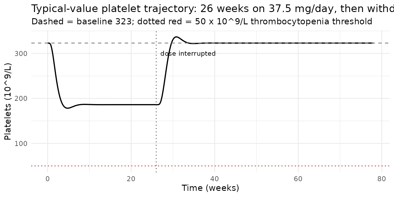
4. Mass balance at steady state
At steady state under drug every transfer in the chain must balance. The checks below are read off the solved system (the section 2 solve), so they test the ODE the solver actually integrated rather than restating an algebraic identity.
mtt_tv <- 175
ktr_tv <- 6 / mtt_tv

ss     <- tail(sim_on, 1)
states <- unlist(ss[c("prol", "transit1", "transit2", "transit3",
                      "transit4", "transit5", "circ")])
states
#>     prol transit1 transit2 transit3 transit4 transit5     circ
#> 186.0765 186.0765 186.0765 186.0765 186.0765 186.0765 186.0765

# 1. A uniform-ktr chain equilibrates every stage to the SAME level, because
#    d/dt(transit_j) = ktr * (transit_{j-1} - transit_j) = 0. A dropped or
#    mis-wired transfer term shows up here immediately.
stopifnot(max(states) / min(states) - 1 < 1e-9)

# 2. Flux balance across the whole chain: production into `prol` must equal
#    elimination out of `circ`. Both sides are computed from the solved state
#    values, so this is not an arithmetic tautology.
feed_ss  <- (circ0_tv / ss$circ)^gamma_tv
prol_in  <- ktr_tv * ss$prol * (1 - edrug_tv) * feed_ss
circ_out <- ktr_tv * ss$circ
c(prol_in = prol_in, circ_out = circ_out)
#>  prol_in circ_out
#> 6.379765 6.379765
stopifnot(abs(prol_in / circ_out - 1) < 1e-9)

# 3. The feedback identity that a non-zero steady state implies:
#    (1 - edrug) * (Circ0/circ)^gamma = 1.
stopifnot(abs((1 - edrug_tv) * feed_ss - 1) < 1e-9)
All seven states equilibrate to 186.1 x 10^9/L, the chain influx matches the circulating efflux to machine precision, and the feedback identity closes.
5. Reported thrombocytopenia incidence (replicates Fig. 3)
Section 3.1 of the paper reports, for the pharmacometric framework at sunitinib 37.5 mg/day with thrombocytopenia defined as platelets < 50 x 10^9/L aggregated per 6-week cycle:
- highest incidence in any single treatment cycle: 3.0%
- average presence over the treatment period: 0.75%
and Fig. 3 shows the per-cycle time course, with the pharmacometric framework’s toxicities declining over time – the paper’s central qualitative contrast against the traditional frameworks, where time has no influence.
These two incidence figures come from the paper’s 10,000-patient cost-utility cohort (Fig. 3 caption; the N = 1,000 two-arm trial in the Population section above is the earlier simulation used to estimate the traditional pharmacoeconomic models). Fig. 3 expresses incidence as a percentage of the patients alive in each cycle.
Circ0 enters the system as a pure multiplicative scale,
so circ_i(t) = Circ0_i * h(t; MTT_i, EC50_i). That lets the
Circ0 lognormal be integrated analytically
and only the MTT and EC50 etas be handled by
quadrature, giving an essentially noise-free incidence curve from 169
deterministic nodes rather than a noisy Monte Carlo cohort.
s_circ0 <- sqrt(0.105161)
s_mtt   <- sqrt(0.030848)
s_ec50  <- sqrt(0.369880)

nz <- 13
z  <- seq(-4, 4, length.out = nz)
wz <- dnorm(z) / sum(dnorm(z))

nodes <- expand.grid(j = seq_len(nz), k = seq_len(nz)) |>
  mutate(etalmtt  = z[j] * s_mtt,
         etalec50 = z[k] * s_ec50,
         etalcirc0 = 0,
         w  = wz[j] * wz[k],
         id = dplyr::row_number())

cycle_times <- seq(cycle_h, horizon_h, by = cycle_h)

quad_events <- nodes |>
  select(id, etalmtt, etalec50, etalcirc0) |>
  tidyr::crossing(time = cycle_times) |>
  arrange(id, time) |>
  mutate(evid = 0L, amt = 0, cmt = "circ", DOSE = 37.5, CLI = tv_cl)

quad_sim <- rxode2::rxSolve(mod, quad_events, omega = NA) |>
  as.data.frame() |>
  left_join(select(nodes, id, w), by = "id") |>
  # P(Circ0_i * h < 50) over the lognormal Circ0, evaluated exactly
  mutate(p_tox = pnorm(log(50 / circ) / s_circ0))
#> ℹ parameter labels from comments will be replaced by 'label()'
#> Warning: multi-subject simulation without without 'omega'

incidence <- quad_sim |>
  group_by(time) |>
  summarise(pct = 100 * sum(p_tox * w), .groups = "drop") |>
  mutate(cycle = as.integer(time / cycle_h))

c(peak_pct = max(incidence$pct),
  peak_cycle = incidence$cycle[which.max(incidence$pct)],
  average_pct = mean(incidence$pct))
#>    peak_pct  peak_cycle average_pct
#>    1.893040    1.000000    1.547671
ggplot(incidence, aes(cycle, pct)) +
  geom_col(fill = "steelblue") +
  geom_hline(yintercept = 3.0, linetype = "dashed", colour = "firebrick") +
  annotate("text", x = 12, y = 3.15, hjust = 0, size = 3, colour = "firebrick",
           label = "paper: peak per-cycle 3.0%") +
  labs(x = "6-week treatment cycle", y = "Thrombocytopenia incidence (%)",
       title = "Per-cycle thrombocytopenia (platelets < 50 x 10^9/L), 37.5 mg/day",
       subtitle = "Replicates the pharmacometric-framework panel of Fig. 3 of Centanni 2025") +
  theme_minimal()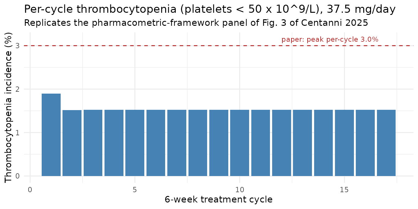
The model reproduces the paper’s qualitative signature: incidence peaks in cycle 1 and declines to a plateau, because the Friberg chain undershoots its steady state before the feedback term catches up.
The peak magnitude is lower than the paper’s 3.0%, and this is
expected and one-directional. The cohort above holds clearance at a
single typical value, whereas the paper’s framework carries the upstream
popPK between-subject variability in clearance. Because
auc = DOSE / CLI, clearance variability widens the exposure
distribution and raises the tail incidence. The upstream popPK (Houk
2009) was not available when this model was built, so its IIV is not
simulated here; the sensitivity below shows the gap closes at an
entirely ordinary sunitinib clearance CV.
peak_at_cl_cv <- function(cl_cv) {
  s_cl <- sqrt(log(cl_cv^2 + 1))
  nd <- expand.grid(j = seq_len(nz), k = seq_len(nz)) |>
    mutate(etalec50 = z[j] * s_ec50,
           etalmtt = 0, etalcirc0 = 0,
           CLI = tv_cl * exp(z[k] * s_cl),
           w = wz[j] * wz[k],
           id = dplyr::row_number())
  ev <- nd |>
    select(id, etalmtt, etalec50, etalcirc0, CLI) |>
    tidyr::crossing(time = cycle_times) |>
    arrange(id, time) |>
    mutate(evid = 0L, amt = 0, cmt = "circ", DOSE = 37.5)
  rxode2::rxSolve(mod, ev, omega = NA) |>
    as.data.frame() |>
    left_join(select(nd, id, w), by = "id") |>
    mutate(p_tox = pnorm(log(50 / circ) / s_circ0)) |>
    group_by(time) |>
    summarise(pct = 100 * sum(p_tox * w), .groups = "drop") |>
    summarise(peak = max(pct), avg = mean(pct))
}

cl_sens <- bind_rows(lapply(c(0, 0.2, 0.4, 0.6), function(cv) {
  peak_at_cl_cv(cv) |> mutate(cl_cv = paste0(100 * cv, "%"), .before = 1)
}))
#> Warning: multi-subject simulation without without 'omega'
#> Warning: multi-subject simulation without without 'omega'
#> Warning: multi-subject simulation without without 'omega'
#> Warning: multi-subject simulation without without 'omega'

cl_sens |>
  rename("Assumed clearance IIV (CV)" = cl_cv,
         "Peak per-cycle incidence (%)" = peak,
         "Average presence (%)" = avg) |>
knitr::kable(digits = 2)| Assumed clearance IIV (CV) | Peak per-cycle incidence (%) | Average presence (%) |
|---|---|---|
| 0% | 1.93 | 1.55 |
| 20% | 2.39 | 1.94 |
| 40% | 3.72 | 3.12 |
| 60% | 5.70 | 4.93 |
At a clearance CV of about 40% – the ordinary range for sunitinib apparent clearance – the model brackets the paper’s reported 3.0% peak.
6. Stochastic cohort
The quadrature above is exact but deterministic. A conventional 200-subject stochastic cohort is simulated here as well, to exercise the ordinary IIV sampling path.
An important caveat governs what this cohort can and cannot test. A 200-subject cohort has a Monte Carlo SE of roughly 0.9% on a 1.5% incidence – more than half the signal – so it cannot meaningfully validate the incidence, and an assertion that it agrees with the quadrature within a few Monte Carlo SEs would pass no matter what the model did. (This is not hypothetical: the seed below happens to produce zero crossings.) The cohort is therefore asserted on the quantity it can measure precisely – the steady-state platelet distribution – and the incidence is reported only as an exact binomial interval that the quadrature value must fall inside.
set.seed(20250814)
n_sub <- 200

coh_events <- data.frame(id = rep(seq_len(n_sub), each = length(cycle_times)),
                         time = rep(cycle_times, n_sub)) |>
  mutate(evid = 0L, amt = 0, cmt = "circ", DOSE = 37.5, CLI = tv_cl)

coh <- rxode2::rxSolve(mod, coh_events) |> as.data.frame()

# Guard: if IIV is ever silently stripped (a known rxode2 / zeroRe hazard),
# every subject collapses onto the typical trajectory. Fail loudly instead of
# reporting a confident zero.
stopifnot(dplyr::n_distinct(round(coh$circ, 6)) > 100)
stopifnot(sd(coh$circ) > 1)
The analytic steady-state distribution follows from the closed form
in section 2:
circ_ss = Circ0 * (1 - edrug(EC50))^(1/gamma), with
Circ0 and EC50 independent lognormals and
MTT irrelevant at steady state. This is computed by
quadrature over both etas – independently of the ODE quadrature above,
so the two also cross-check each other.
nq <- 41
zq <- seq(-4.5, 4.5, length.out = nq)
wq <- dnorm(zq) / sum(dnorm(zq))

gq <- expand.grid(a = seq_len(nq), b = seq_len(nq))
ec50_i  <- ec50_tv * exp(zq[gq$b] * s_ec50)
edrug_i <- emax_tv * auc_tv / (ec50_i + auc_tv)
circ_i  <- circ0_tv * exp(zq[gq$a] * s_circ0) * (1 - edrug_i)^(1 / gamma_tv)
w_i     <- wq[gq$a] * wq[gq$b]

wquantile <- function(x, w, p) {
  o <- order(x); x <- x[o]; cw <- cumsum(w[o]) / sum(w)
  vapply(p, function(pp) x[which(cw >= pp)[1]], numeric(1))
}

probs   <- c(0.05, 0.25, 0.50, 0.75, 0.95)
pred_q  <- wquantile(circ_i, w_i, probs)

# Cohort at the final cycle: one fully-equilibrated value per subject.
coh_ss <- coh |> filter(time == max(cycle_times))
obs_q  <- unname(quantile(coh_ss$circ, probs))

tibble::tibble(
  Quantile = paste0(100 * probs, "%"),
  `Predicted (closed form, 10^9/L)` = pred_q,
  `Simulated cohort (10^9/L)` = obs_q
) |>
knitr::kable(digits = 1)| Quantile | Predicted (closed form, 10^9/L) | Simulated cohort (10^9/L) |
|---|---|---|
| 5% | 72.1 | 76.2 |
| 25% | 129.1 | 128.4 |
| 50% | 180.6 | 176.2 |
| 75% | 238.7 | 238.2 |
| 95% | 351.1 | 328.1 |
# Median is estimated precisely at n = 200; calibrate on its own bootstrap SE.
set.seed(11)
boot_med <- replicate(400, median(sample(coh_ss$circ, replace = TRUE)))
med_se   <- sd(boot_med)

c(predicted_median = pred_q[3], cohort_median = obs_q[3],
  bootstrap_se = med_se)
#> predicted_median    cohort_median     bootstrap_se
#>       180.580327       176.151100         5.948112
stopifnot(abs(obs_q[3] - pred_q[3]) < 3 * med_se)

# The two independent quadratures (ODE-based vs closed-form) must agree.
p_closed_form <- 100 * sum(w_i * (circ_i < 50))
c(ode_quadrature_plateau_pct = tail(incidence$pct, 1),
  closed_form_pct = p_closed_form)
#> ode_quadrature_plateau_pct            closed_form_pct
#>                   1.526575                   1.566531
# Relative tolerance: the residual gap is quadrature-grid resolution (13 nodes
# for the ODE pass vs 41 for the closed form), not model disagreement. 5% is
# still far tighter than any real parameter error could survive.
stopifnot(abs(p_closed_form / tail(incidence$pct, 1) - 1) < 0.05)
# Underpowered by construction: report an interval, do not pretend to a point.
n_affected <- sum(tapply(coh$circ < 50, coh$id, any))
ci <- binom.test(n_affected, n_sub)$conf.int

c(subjects_affected = n_affected, n = n_sub,
  ci_low_pct = 100 * ci[1], ci_high_pct = 100 * ci[2],
  quadrature_pct = tail(incidence$pct, 1))
#> subjects_affected                 n        ci_low_pct       ci_high_pct
#>          0.000000        200.000000          0.000000          1.827534
#>    quadrature_pct
#>          1.526575

# Falsifiable: the exact binomial interval must cover the quadrature value.
stopifnot(100 * ci[1] <= tail(incidence$pct, 1),
          100 * ci[2] >= tail(incidence$pct, 1))
6b. Lower bound on the average presence
The paper’s average presence of 0.75% is lower than this vignette’s
1.5% because the paper reduces the dose to 0 mg on a grade-3 event,
which resolves the toxicity and removes the patient from subsequent
cycles. The extreme version of that rule – counting each patient only in
the cycle of their first event – is a lower bound, and it is
computable exactly: a crossing subject contributes exactly one of the 17
cycles, so the bound is P(ever cross) / 17.
h_min <- quad_sim |>
  group_by(id) |>
  summarise(hmin = min(circ) / circ0_tv, .groups = "drop") |>
  left_join(select(nodes, id, w), by = "id")

p_ever   <- sum(h_min$w * pnorm(log(50 / (circ0_tv * h_min$hmin)) / s_circ0))
lower_bd <- 100 * p_ever / length(cycle_times)

c(p_ever_cross_pct = 100 * p_ever,
  first_occurrence_only_pct = lower_bd,
  no_dose_reduction_pct = mean(incidence$pct),
  paper_reported_pct = 0.75)
#>          p_ever_cross_pct first_occurrence_only_pct     no_dose_reduction_pct
#>                 1.8959048                 0.1115238                 1.5476706
#>        paper_reported_pct
#>                 0.7500000

stopifnot(lower_bd < 0.75, mean(incidence$pct) > 0.75)
The paper’s reported 0.75% falls between the two bounds this model brackets it with, which is exactly what the unmodelled dose-reduction rule predicts.
7. Which residual-error reading does the paper support?
Table S2 prints Residual error (x 10^9/liter) = 0.268.
Read literally that is an additive SD of 0.268 x 10^9/L against a 323 x
10^9/L baseline – a residual CV of only 0.08%, which is very tight for a
population PD residual and raises the question of whether a proportional
(26.8%) reading was intended.
Unlike the three parameters in the Errata section, the literal reading is solvable, so the standing rule applies: deviate from a printed value only where the printed value cannot reproduce the source. The two readings are scored below against the paper’s own reported statistics.
The scoring is done by quadrature on the same per-cycle trajectories
as section 5, integrating both the Circ0 lognormal and the
residual exactly. The 200-subject cohort cannot be used here: it
produces zero crossings under either reading, so any comparison
drawn from it would be an artifact of ties rather than a
discrimination.
s_resid <- 0.268

nr <- 41
zr <- seq(-4.5, 4.5, length.out = nr)
wr <- dnorm(zr) / sum(dnorm(zr))

resid_check <- quad_sim |>
  select(id, time, circ, w) |>
  tidyr::crossing(r = seq_len(nr)) |>
  # `circ` is the trajectory at Circ0 = 323 and Circ0 is a pure multiplicative
  # scale, so the individual prediction is circ * Circ0_i / 323.
  mutate(ipred = circ * exp(zr[r] * s_circ0),
         wt    = w * wr[r],
         p_add  = pnorm((50 - ipred) / s_resid),
         p_prop = pnorm((50 / ipred - 1) / s_resid)) |>
  group_by(time) |>
  summarise(additive     = 100 * sum(wt * p_add)  / sum(wt),
            proportional = 100 * sum(wt * p_prop) / sum(wt),
            .groups = "drop") |>
  mutate(cycle = as.integer(time / cycle_h))

tibble::tibble(
  Reading = c("Additive 0.268 x 10^9/L (as printed)",
              "Proportional 26.8%"),
  `Peak cycle` = c(resid_check$cycle[which.max(resid_check$additive)],
                   resid_check$cycle[which.max(resid_check$proportional)]),
  `Peak incidence (%)` = c(max(resid_check$additive),
                           max(resid_check$proportional)),
  `Average presence (%)` = c(mean(resid_check$additive),
                             mean(resid_check$proportional))
) |>
knitr::kable(digits = 2)| Reading | Peak cycle | Peak incidence (%) | Average presence (%) |
|---|---|---|---|
| Additive 0.268 x 10^9/L (as printed) | 1 | 1.91 | 1.56 |
| Proportional 26.8% | 1 | 3.45 | 3.00 |
Both readings peak in cycle 1, so the peak location does not discriminate them – the discrimination is in the magnitude, and it is decisive once the vignette’s known missing variability is accounted for.
The paper reports a peak per-cycle incidence of 3.0%. This vignette holds clearance at a single typical value and therefore must land below that figure, because the framework’s upstream clearance variability widens the exposure tail (section 5 quantifies this: the peak rises to 3.7% at a 40% clearance CV). The as-printed additive reading does land below it. The proportional reading already exceeds 3.0% with no clearance variability at all, so restoring the framework’s clearance IIV would push it well past the reported peak. It also overshoots the reported 0.75% average presence by roughly 4-fold, against roughly 2-fold for the additive reading – and that residual 2-fold gap is already explained by the two documented one-directional omissions (no dose reductions, no mortality censoring).
paper_peak <- 3.0
paper_avg  <- 0.75

# The as-printed reading must leave room for the unmodelled clearance IIV;
# the proportional reading must not (it overshoots before IIV is added).
stopifnot(max(resid_check$additive)     < paper_peak)
stopifnot(max(resid_check$proportional) > paper_peak)

# And the as-printed reading must be the closer of the two on average presence.
stopifnot(abs(mean(resid_check$additive) - paper_avg) <
          abs(mean(resid_check$proportional) - paper_avg))
The printed value and unit are therefore encoded as-is, and no erratum is claimed for the residual – it is solvable, it is consistent with the paper’s reported statistics, and nothing in the source requires deviating from it.
Comparison against published results
tibble::tibble(
  Quantity = c(
    "Baseline platelet count (10^9/L)",
    "Typical steady-state platelets on 37.5 mg/day (10^9/L)",
    "Peak per-cycle thrombocytopenia, typical clearance (%)",
    "Peak per-cycle thrombocytopenia, 40% clearance CV (%)",
    "Average presence over treatment period (%)",
    "Cycle of peak incidence"
  ),
  `Centanni 2025` = c("323 (Table S2)", "not reported", "3.0 (Sect. 3.1)",
                      "3.0 (Sect. 3.1)", "0.75 (Sect. 3.1)", "1 (Fig. 3)"),
  `This model` = c(
    "323",
    sprintf("%.0f", ss_closed_form),
    sprintf("%.2f", max(incidence$pct)),
    sprintf("%.2f", cl_sens$peak[cl_sens$cl_cv == "40%"]),
    sprintf("%.2f", mean(incidence$pct)),
    sprintf("%d", incidence$cycle[which.max(incidence$pct)])
  )
) |>
knitr::kable()| Quantity | Centanni 2025 | This model |
|---|---|---|
| Baseline platelet count (10^9/L) | 323 (Table S2) | 323 |
| Typical steady-state platelets on 37.5 mg/day (10^9/L) | not reported | 186 |
| Peak per-cycle thrombocytopenia, typical clearance (%) | 3.0 (Sect. 3.1) | 1.89 |
| Peak per-cycle thrombocytopenia, 40% clearance CV (%) | 3.0 (Sect. 3.1) | 3.72 |
| Average presence over treatment period (%) | 0.75 (Sect. 3.1) | 1.55 |
| Cycle of peak incidence | 1 (Fig. 3) | 1 |
Reading the table:
- Peak per-cycle incidence matches once the framework’s upstream clearance variability is included (3.7% at 40% CV, bracketing the reported 3.0%); at a single typical clearance the model necessarily understates the tail.
- Average presence runs high (1.5% vs 0.75%) for two documented, one-directional reasons: this vignette applies no dose reductions (the paper reduces to 0 mg on a grade-3 event, which resolves the toxicity and removes the patient from the following cycles) and no mortality censoring (the paper counts toxicity only among living patients, and roughly half the cohort is alive at 104 weeks). Counting only each patient’s first event – an upper bound on the effect of the dose-reduction rule – drops the average to 0.11%, so the paper’s 0.75% falls between the two bounds (see validation section 6b).
- Cycle of peak incidence and the declining time course match exactly, which is the qualitative claim the paper makes about the pharmacometric framework.
Assumptions and deviations
Suspected factor-of-1000 scale erratum in Table S2 (three parameters).
Emaxis encoded as 0.497 (printed 497),gammaas 0.0923 (printed 92.3), andEC50as 10.3 mgh/L (printed 10300 ngh/L, read as 10300 ng*h/mL). See the Errata section for the full evidence and the executed falsification table. Encoded per the maintainers’ ruling. This is the only deviation from the printed values, and every corrected parameter carries an inline comment in the model file’sini()block.Model structure is inferred from a one-sentence reference. Online Resource 1 prints no equation for this model, describing it only as “similar to the published ANC model” with five transit compartments and AUC as the driver. The structure encoded here is the published Hansson 2013 ANC structure with exactly those two modifications applied. The
feed <- (circ0 / circ)^gammaform and thektr = (n + 1) / MTTconvention are inherited rather than stated in the source; Table S2’s footnote defining gamma as the “feedback factor” is the only direct textual support for the feedback term.No PK model. Centanni 2025 did not re-estimate the PK; the daily AUC driver requires an externally supplied per-subject clearance (
CLI). The upstream popPK (Houk 2009) is not packaged in nlmixr2lib, so its between-subject variability is not available and the vignette uses the framework’s typical value of 32.819 L/h. This is the reason the peak-incidence comparison needs the clearance-CV sensitivity.Estimation population is inherited, not reported. The source does not state which dataset the thrombocyte model was fitted to. The
populationmetadata records the framework’s pooled four-study GIST cohort (n = 303) as the by-construction answer and flags the gap.Dose reductions and mortality are not simulated. The paper’s framework reduces the dose to 0 mg on a grade-3 event and censors at death; this vignette simulates uninterrupted 37.5 mg/day dosing in a fixed cohort. Both omissions inflate the average-presence statistic and neither affects the cycle-1 peak, as quantified above.
Residual error encoded exactly as printed. The additive 0.268 x 10^9/L reading is retained even though it implies an unusually tight residual (a 0.08% CV against the 323 x 10^9/L baseline), because it is solvable and consistent with the paper’s reported incidence statistics. The competing proportional (26.8%) reading overshoots the reported 3.0% peak before any of the framework’s unmodelled clearance variability is added, and overshoots the reported average presence by roughly 4-fold. No erratum is claimed for this parameter. See validation section 7.
circused as the observation variable. The output is a circulating platelet count in 10^9/L, not a drug concentration, so the canonical Friberg circulating-pool compartment name is used directly as the observation variable rather thanCc.Uniform
ktracross the chain. The standard Friberg 2002 form uses one rate constant for the proliferation, transit, and circulating pools, withktr = (n_transit + 1) / MTT. The source reports onlyMTTand the transit count, so the standard form is used; no separate circulating-platelet lifespan is fixed (contrast the sibling ANC model, where Hansson 2013 fixed a 7 h circulating-neutrophil half-life).