Gastric emptying meta-analysis (Bonner 2015)
Source:vignettes/articles/Bonner_2015_gastric_emptying.Rmd
Bonner_2015_gastric_emptying.RmdModel and source
- Citation: Bonner JJ, Vajjah P, Abduljalil K, Jamei M, Rostami-Hodjegan A, Tucker GT, Johnson TN (2015). Does age affect gastric emptying time? A model-based meta-analysis of data from premature neonates through to adults. Biopharm Drug Dispos 36(4):245-57.
- Article: https://doi.org/10.1002/bdd.1937
The packaged model implements the final double Weibull meta-analysis of gastric emptying time (Bonner 2015 Eq. 1) fit to pooled data from 49 published gastric-emptying studies (n = 1457 subjects spanning 28 weeks gestational age preterm neonates through adults up to ~84 years). The model has NO drug, NO dose, and NO PK compartment: the sole modelled quantity is the fraction of a test meal remaining in the stomach as a function of time-after-ingestion. The paper’s key finding is that age was NOT a significant covariate on gastric emptying after allowance for test-meal type, while meal type (a five-way partition into aqueous / breast milk / formula / semi-solid / solid) was the only significant covariate.
Population
n = 1457 subjects across 49 studies (model-development set) plus an independent validation set of 468 subjects across 17 studies. Age range: 28 weeks gestational age (VLBW preterm neonates) through adults up to ~1008 months (~84 years). Sex: mostly not specified in the paediatric subsample (637 / 1132 paediatric subjects had sex unrecorded); of subjects with sex recorded the split is ~50/50. GE measurement methods pooled across scintigraphy (T = 2 in the residual-error weighting), dilution (phenol red or PEG), ultrasound, MRI, and applied potential tomography (T = 1). Test meals administered orally, by nasogastric tube, or by orogastric tube. See supplementary Table 1 of the paper for the per-study breakdown.
The metadata is available programmatically:
mod_meta <- rxode2::rxode2(readModelDb("Bonner_2015_gastric_emptying"))
#> ℹ parameter labels from comments will be replaced by 'label()'
str(mod_meta$population)
#> List of 10
#>  $ species       : chr "human"
#>  $ n_subjects    : int 1457
#>  $ n_studies     : int 49
#>  $ age_range     : chr "28 weeks gestational age (VLBW preterm neonates) through adults up to ~84 years (1008 months). Median across pa"| __truncated__
#>  $ weight_range  : chr "Not reported per-study in the pooled dataset. Population physically spans preterm neonates (<= ~1 kg) through adults."
#>  $ sex_female_pct: chr "Not fully specified across the dataset. Of the 1457 modelling subjects, 637 were paediatrics with sex not speci"| __truncated__
#>  $ regions       : chr "Not reported per-study. 49 modelling studies drawn from PubMed / Embase (English-language, human) published 1975 - 2012."
#>  $ dose_range    : chr "No drug dosing. Test meals administered orally, by nasogastric tube, or by orogastric tube; span 5 - 10% dextro"| __truncated__
#>  $ disease_state : chr "Healthy preterm neonates through adults. Exclusions per Methods: obese subjects, subjects on GI-motility drugs "| __truncated__
#>  $ notes         : chr "Model-development set: n = 1457 subjects across 49 studies. Independent validation set: n = 468 subjects across"| __truncated__
Source trace
The per-parameter origin is recorded in the model file’s
ini() block. The table below collects them for quick
review.
| Equation / parameter | Value | Source location |
|---|---|---|
| Eq. 1: double Weibull structural form | - | Bonner 2015 p. 247, Eq. 1 |
| Eq. 2: exp(eta_i) log-normal IIV | - | Bonner 2015 p. 247, Eq. 2 |
| Eq. 3: weighted additive residual error | - | Bonner 2015 p. 247-248, Eq. 3 |
| Eq. 4: MGRT via AUMC / AUC of the double Weibull | - | Bonner 2015 p. 248, Eq. 4 |
llogit_pr (logit of PR / 100, PR = 0.26%) |
-5.951 | Table 3, “PR (%)” row |
lbeta1 (log fast-phase Weibull shape) |
log(0.816) | Table 3, “beta1” row |
lbeta2 (log slow-phase Weibull shape) |
log(2.48) | Table 3, “beta2” row |
lgamma1 (log fast-phase Weibull scale, min) |
log(37.6) | Table 3, “gamma1 (min)” row |
lgamma2 (log slow-phase Weibull scale, min) |
log(63.7) | Table 3, “gamma2 (min)” row |
ltheta_aq (log aqueous meal coefficient) |
log(0.697) | Table 3, “theta Aqueous” row |
ltheta_bm (log breast-milk meal coefficient) |
log(0.959) | Table 3, “theta Breast milk” row |
ltheta_fm (log formula meal coefficient) |
log(1.15) | Table 3, “theta Form” row |
ltheta_ss (log semi-solid meal coefficient) |
log(1.61) | Table 3, “theta Semi solid” row |
ltheta_sol (log solid meal coefficient) |
log(1.99) | Table 3, “theta Solid” row |
etallogit_pr (BSV logit(PR / 100), interpreted as
CV%) |
0.833 | Table 3, “Variability omega^2” row |
etalbeta1 (BSV beta1, interpreted as CV%) |
0.139 | Table 3, “Variability omega^2” row |
etalbeta2 (BSV beta2, interpreted as CV%) |
0.0197 | Table 3, “Variability omega^2” row |
etalgamma1 (BSV gamma1, interpreted as CV%) |
0.296 | Table 3, “Variability omega^2” row |
etalgamma2 (BSV gamma2, interpreted as CV%) |
0.0362 | Table 3, “Variability omega^2” row |
addSd (weighted additive residual SD theta_w, %) |
11.1 | Table 3, “theta_w” row |
Reported meal-type MGRTs from the paper’s 1000-individual simulation (Bonner 2015 Results, p. 250): 45 min (aqueous), 57 min (breast milk), 64 min (formula), 87 min (semi-solid), 98 min (solid). Reference: Figure 3 box-whisker plot.
Simulation setup
The model is purely algebraic (double Weibull evaluated at each
observation time; no ODEs). Each of the five test-meal categories is
encoded as a mutually-exclusive binary covariate
(MEAL_AQUEOUS, MEAL_BREASTMILK,
MEAL_FORMULA, MEAL_SEMISOLID,
MEAL_SOLID). Exactly one of the five indicators is
1 per record; the remaining four are 0. There
is no dosing event, no drug, and no plasma compartment.
mod <- readModelDb("Bonner_2015_gastric_emptying")
ui  <- rxode2::rxode2(mod)
#> ℹ parameter labels from comments will be replaced by 'label()'
ui
#>  ── rxode2-based Pred model ─────────────────────────────────────────────────────
#>  ── Initalization: ──
#> Fixed Effects ($theta):
#>  llogit_pr     lbeta1     lbeta2    lgamma1    lgamma2  ltheta_aq  ltheta_bm
#> -5.9496404 -0.2033409  0.9082586  3.6270041  4.1541846 -0.3609699 -0.0418642
#>  ltheta_fm  ltheta_ss ltheta_sol      addSd
#>  0.1397619  0.4762342  0.6881346 11.1000000
#>
#> Omega ($omega):
#>              etallogit_pr etalbeta1 etalbeta2 etalgamma1 etalgamma2
#> etallogit_pr        0.833     0.000    0.0000      0.000     0.0000
#> etalbeta1           0.000     0.139    0.0000      0.000     0.0000
#> etalbeta2           0.000     0.000    0.0197      0.000     0.0000
#> etalgamma1          0.000     0.000    0.0000      0.296     0.0000
#> etalgamma2          0.000     0.000    0.0000      0.000     0.0362
#> attr(,"lotriLabels")
#> [1] "Table 3: omega^2 PR    = 114  -> CV = 114% -> log(1 + 1.14^2)   = 0.833"
#> [2] "Table 3: omega^2 beta1 = 38.6 -> CV = 38.6% -> log(1 + 0.386^2) = 0.139"
#> [3] "Table 3: omega^2 beta2 = 14.1 -> CV = 14.1% -> log(1 + 0.141^2) = 0.0197"
#> [4] "Table 3: omega^2 gamma1 = 58.7 -> CV = 58.7% -> log(1 + 0.587^2) = 0.296"
#> [5] "Table 3: omega^2 gamma2 = 19.2 -> CV = 19.2% -> log(1 + 0.192^2) = 0.0362"
#> attr(,"lotriFix")
#>              etallogit_pr etalbeta1 etalbeta2 etalgamma1 etalgamma2
#> etallogit_pr        FALSE     FALSE     FALSE      FALSE      FALSE
#> etalbeta1           FALSE     FALSE     FALSE      FALSE      FALSE
#> etalbeta2           FALSE     FALSE     FALSE      FALSE      FALSE
#> etalgamma1          FALSE     FALSE     FALSE      FALSE      FALSE
#> etalgamma2          FALSE     FALSE     FALSE      FALSE      FALSE
#>  ── μ-referencing ($muRefTable): ──
#>       theta          eta level
#> 1    lbeta1    etalbeta1    id
#> 2    lbeta2    etalbeta2    id
#> 3   lgamma1   etalgamma1    id
#> 4   lgamma2   etalgamma2    id
#> 5 llogit_pr etallogit_pr    id
#>
#>  ── Model (Normalized Syntax): ──
#> function() {
#>     covariateData <- list(MEAL_AQUEOUS = list(description = "Binary indicator for aqueous test meal (water, sugar solutions, fruit juice per Bonner 2015 Methods 'Covariate selection and evaluation'). 1 = aqueous test meal for the study record; 0 = otherwise. Selects theta_Aqueous in the meal-type mixture; because aqueous is the renormalised reference (theta_meal / theta_Aqueous), MEAL_AQUEOUS = 1 gives a meal-type ratio of exactly 1 on gamma1 for that record.",
#>         units = "(binary)", type = "binary", reference_category = "0 (not aqueous)",
#>         notes = "Bonner 2015 Table 3 theta_Aqueous = 0.697. Mutually exclusive with MEAL_BREASTMILK, MEAL_FORMULA, MEAL_SEMISOLID, MEAL_SOLID -- exactly one of the five MEAL_* indicators is 1 per record. See vignette Errata for the meal-type attachment-point best-effort choice (multiplies gamma1 with aqueous as the renormalised reference).",
#>         source_name = "aqueous solution"), MEAL_BREASTMILK = list(description = "Binary indicator for breast-milk test meal. 1 = breast milk; 0 = otherwise. Multiplicative scaling factor on the fast-phase Weibull scale gamma1.",
#>         units = "(binary)", type = "binary", reference_category = "0 (not breast milk)",
#>         notes = "Bonner 2015 Table 3 theta_Breast_milk = 0.959. Mutually exclusive with the other MEAL_* indicators.",
#>         source_name = "breast milk"), MEAL_FORMULA = list(description = "Binary indicator for formula (any variety, including nutritional shakes per Methods).",
#>         units = "(binary)", type = "binary", reference_category = "0 (not formula)",
#>         notes = "Bonner 2015 Table 3 theta_Form = 1.15. Mutually exclusive with the other MEAL_* indicators.",
#>         source_name = "formula"), MEAL_SEMISOLID = list(description = "Binary indicator for semi-solid meal (pudding, rice cereal, or oatmeal per Methods).",
#>         units = "(binary)", type = "binary", reference_category = "0 (not semi-solid)",
#>         notes = "Bonner 2015 Table 3 theta_Semi_solid = 1.61. Mutually exclusive with the other MEAL_* indicators.",
#>         source_name = "semi-solid meals"), MEAL_SOLID = list(description = "Binary indicator for solid meal (e.g., pancakes, eggs, chicken liver, sandwich meals per Bonner 2015 supplementary Table 1).",
#>         units = "(binary)", type = "binary", reference_category = "0 (not solid)",
#>         notes = "Bonner 2015 Table 3 theta_Solid = 1.99. Mutually exclusive with the other MEAL_* indicators.",
#>         source_name = "solid meals"))
#>     covariatesDataExcluded <- list(PNA = list(description = "Postnatal age in weeks. Tested as a covariate on GE (paper Methods 'Covariate selection and evaluation') after allowance for meal type and rejected because the objective function value did not change materially: BASE MODEL + Food types + postnatal Age OFV 1875.121 vs Food types alone OFV 1875.252 (Table 2), delta OFV = -0.13, not significant. Documented here so downstream users know age was screened.",
#>         units = "weeks", type = "continuous", reference_category = NULL,
#>         notes = "Screened per Methods; not retained in the final model. Postmenstrual age (postnatal + gestational, in weeks) was used only for graphical purposes and not as a modelled covariate."),
#>         GA = list(description = "Gestational age at birth in weeks. Tested as a covariate on GE after allowance for meal type (paper Table 2: BASE MODEL + Food types + Gestational age OFV 1875.211 vs Food types alone 1875.252, delta OFV = -0.04). Rejected as non-significant.",
#>             units = "weeks", type = "continuous", reference_category = NULL,
#>             notes = "Same rationale as PNA: screened per Methods, not retained. For preterm neonates gestational age at birth was added to postnatal age when computing postmenstrual age for graphical inspection."))
#>     description <- "Population meta-analysis of the postprandial gastric emptying (GE) time course in humans, pooled across 49 published studies of 1457 subjects spanning 28 weeks gestational age (very-low-birth- weight preterm neonates) through adults (Bonner 2015). Structural model is a double Weibull mixture on the fraction of test meal remaining in the stomach vs. time-after-ingestion (Eq. 1: GE = (100 - PR) * exp(-(t/gamma1)^beta1) + PR * exp(-(t/gamma2)^beta2)). The five test meal categories (aqueous, breast milk, formula, semi-solid, solid) are the only significant covariate; postnatal age and gestational age were tested and found NOT significant. The five reported theta_meal coefficients enter as multiplicative scalings on the fast-phase Weibull scale gamma1, with aqueous as the renormalised reference (theta_meal / theta_Aqueous). This attachment point, the natural- percent reading of PR, and the CV-percent reading of the Table 3 omega^2 column are documented best-effort interpretations because the paper's Methods do not specify which parameter the meal-type theta modifies, the PR reporting scale, or the omega^2 unit convention, and neither the main paper nor the two supplementary material files contain the NONMEM control stream. See the validation vignette's Errata for the full ambiguity list and the best-effort choices approved by the maintainers. Not a drug PK model -- no dose, no plasma compartment, no drug PK observation; the single state is the percentage of test meal remaining, initialised to 100 at t = 0 by construction. Reported meal-type mean gastric residence times (MGRT, Eq. 4) from the paper's 1000-individual simulations: 45 min (aqueous), 57 min (breast milk), 64 min (formula), 87 min (semi-solid), 98 min (solid)."
#>     paper_specific_compartments <- "gastric_remaining"
#>     population <- list(species = "human", n_subjects = 1457L,
#>         n_studies = 49L, age_range = "28 weeks gestational age (VLBW preterm neonates) through adults up to ~84 years (1008 months). Median across paediatric studies is low (many neonatal / preterm cohorts); adult subjects (325 individuals) span ~17-84 years. See supplementary Table 1 for the per-study 'Age in months mean (range)' column.",
#>         weight_range = "Not reported per-study in the pooled dataset. Population physically spans preterm neonates (<= ~1 kg) through adults.",
#>         sex_female_pct = "Not fully specified across the dataset. Of the 1457 modelling subjects, 637 were paediatrics with sex not specified; 495 paediatrics with sex specified (256 M / 228 F, plus 11 not-clearly-classified); 325 adults with sex specified (160 M / 165 F). The 165 adult women include both pre- and postmenopausal ages; most studies did not distinguish.",
#>         regions = "Not reported per-study. 49 modelling studies drawn from PubMed / Embase (English-language, human) published 1975 - 2012.",
#>         dose_range = "No drug dosing. Test meals administered orally, by nasogastric tube, or by orogastric tube; span 5 - 10% dextrose / sugar solutions, breast milk, term / preterm infant formula, rice cereal / pudding, pancakes, egg sandwiches, chicken liver, and other solids (see supplementary Table 1 for the per-study test-meal detail).",
#>         disease_state = "Healthy preterm neonates through adults. Exclusions per Methods: obese subjects, subjects on GI-motility drugs (e.g., metoclopramide, cisapride), any disease other than apnoea, and subjects with confirmed gastro-oesophageal reflux (subjects referred for suspected GOR were retained).",
#>         notes = "Model-development set: n = 1457 subjects across 49 studies. Independent validation set: n = 468 subjects across 17 studies (marked '*' in supplementary Table 1). Sampling times 20 - 300 min after meal ingestion; time-points-per-study ranged 1 - 19 (many single-time-point neonatal studies); subjects-per-study ranged 6 - 186. GE measurement methods pooled across scintigraphy (Tc-99m or In-111 -- residual-error weight T = 2), dilution (phenol red or polyethylene glycol), ultrasound, MRI, and applied potential tomography (T = 1). PR is estimated on a logit-transformed scale to keep the parameter in (0, 100). Fit in NONMEM 7.2 with FOCE-I.")
#>     reference <- "Bonner JJ, Vajjah P, Abduljalil K, Jamei M, Rostami-Hodjegan A, Tucker GT, Johnson TN. Does age affect gastric emptying time? A model-based meta-analysis of data from premature neonates through to adults. Biopharm Drug Dispos. 2015 May;36(4):245-57. doi:10.1002/bdd.1937."
#>     units <- list(time = "min", dosing = "none (the % remaining is initialised to 100 at t = 0 by construction of Eq. 1; test meal is not represented as a dose)",
#>         concentration = "% of test meal remaining in the stomach (0 - 100)")
#>     vignette <- "Bonner_2015_gastric_emptying"
#>     ini({
#>         llogit_pr <- -5.94964044808459
#>         label("Logit of the fast-phase-completed remaining fraction PR/100 (unitless; logit(0.0026) = -5.951)")
#>         lbeta1 <- -0.20334092401803
#>         label("Log of the fast-phase Weibull shape beta1 (unitless)")
#>         lbeta2 <- 0.908258560176891
#>         label("Log of the slow-phase Weibull shape beta2 (unitless)")
#>         lgamma1 <- 3.62700405039585
#>         label("Log of the fast-phase Weibull scale gamma1 (min)")
#>         lgamma2 <- 4.15418456257812
#>         label("Log of the slow-phase Weibull scale gamma2 (min)")
#>         ltheta_aq <- -0.360969868221613
#>         label("Log of the aqueous test-meal coefficient theta_Aqueous (unitless)")
#>         ltheta_bm <- -0.0418642040986989
#>         label("Log of the breast-milk test-meal coefficient theta_Breast_milk (unitless)")
#>         ltheta_fm <- 0.139761942375159
#>         label("Log of the formula test-meal coefficient theta_Form (unitless)")
#>         ltheta_ss <- 0.476234178996372
#>         label("Log of the semi-solid test-meal coefficient theta_Semi_solid (unitless)")
#>         ltheta_sol <- 0.688134638736401
#>         label("Log of the solid test-meal coefficient theta_Solid (unitless)")
#>         addSd <- c(0, 11.1)
#>         label("Weighted-additive residual SD theta_w (% remaining); Eq. 3 N * T weighting NOT reproduced")
#>         etallogit_pr ~ 0.833
#>         label("Table 3: omega^2 PR    = 114  -> CV = 114% -> log(1 + 1.14^2)   = 0.833")
#>         etalbeta1 ~ 0.139
#>         label("Table 3: omega^2 beta1 = 38.6 -> CV = 38.6% -> log(1 + 0.386^2) = 0.139")
#>         etalbeta2 ~ 0.0197
#>         label("Table 3: omega^2 beta2 = 14.1 -> CV = 14.1% -> log(1 + 0.141^2) = 0.0197")
#>         etalgamma1 ~ 0.296
#>         label("Table 3: omega^2 gamma1 = 58.7 -> CV = 58.7% -> log(1 + 0.587^2) = 0.296")
#>         etalgamma2 ~ 0.0362
#>         label("Table 3: omega^2 gamma2 = 19.2 -> CV = 19.2% -> log(1 + 0.192^2) = 0.0362")
#>     })
#>     model({
#>         beta1_i <- exp(lbeta1 + etalbeta1)
#>         beta2_i <- exp(lbeta2 + etalbeta2)
#>         gamma1_i <- exp(lgamma1 + etalgamma1)
#>         gamma2_i <- exp(lgamma2 + etalgamma2)
#>         logit_pr_i <- llogit_pr + etallogit_pr
#>         pr_frac_i <- expit(logit_pr_i, 0, 1)
#>         pr_pct_i <- 100 * pr_frac_i
#>         theta_meal_raw <- exp(ltheta_aq) * MEAL_AQUEOUS + exp(ltheta_bm) *
#>             MEAL_BREASTMILK + exp(ltheta_fm) * MEAL_FORMULA +
#>             exp(ltheta_ss) * MEAL_SEMISOLID + exp(ltheta_sol) *
#>             MEAL_SOLID
#>         theta_meal_ratio <- theta_meal_raw/exp(ltheta_aq)
#>         gamma1_eff <- gamma1_i * theta_meal_ratio
#>         t_eff <- time + 1e-09
#>         gastric_remaining <- (100 - pr_pct_i) * exp(-(t_eff/gamma1_eff)^beta1_i) +
#>             pr_pct_i * exp(-(t_eff/gamma2_i)^beta2_i)
#>         gastric_remaining ~ add(addSd)
#>     })
#> }
one_meal_event_table <- function(meal, times) {
  et <- as.data.frame(rxode2::et(times))
  et$MEAL_AQUEOUS    <- as.integer(meal == "aqueous")
  et$MEAL_BREASTMILK <- as.integer(meal == "breastmilk")
  et$MEAL_FORMULA    <- as.integer(meal == "formula")
  et$MEAL_SEMISOLID  <- as.integer(meal == "semisolid")
  et$MEAL_SOLID      <- as.integer(meal == "solid")
  et
}
Typical-value gastric-emptying curves by meal type
The typical-value simulation (rxode2::zeroRe(ui))
reproduces the paper’s Figure 2 / Figure 3 pattern that aqueous meals
empty fastest and solid meals slowest, with breast milk / formula /
semi-solid falling in between.
times <- seq(0, 300, by = 1)
meals <- c("aqueous", "breastmilk", "formula", "semisolid", "solid")
sim_typ <- lapply(meals, function(mt) {
  et <- one_meal_event_table(mt, times)
  s  <- rxode2::rxSolve(rxode2::zeroRe(ui), events = et, nSub = 1)
  data.frame(
    meal              = mt,
    time              = as.data.frame(s)$time,
    gastric_remaining = as.data.frame(s)$gastric_remaining
  )
})
#> ℹ omega/sigma items treated as zero: 'etallogit_pr', 'etalbeta1', 'etalbeta2', 'etalgamma1', 'etalgamma2'
#> ℹ omega/sigma items treated as zero: 'etallogit_pr', 'etalbeta1', 'etalbeta2', 'etalgamma1', 'etalgamma2'
#> ℹ omega/sigma items treated as zero: 'etallogit_pr', 'etalbeta1', 'etalbeta2', 'etalgamma1', 'etalgamma2'
#> ℹ omega/sigma items treated as zero: 'etallogit_pr', 'etalbeta1', 'etalbeta2', 'etalgamma1', 'etalgamma2'
#> ℹ omega/sigma items treated as zero: 'etallogit_pr', 'etalbeta1', 'etalbeta2', 'etalgamma1', 'etalgamma2'
sim_typ <- dplyr::bind_rows(sim_typ)
ggplot(sim_typ, aes(time, gastric_remaining, colour = meal)) +
  geom_line(size = 0.9) +
  scale_colour_manual(
    values = c(aqueous = "black", breastmilk = "royalblue",
               formula = "forestgreen", semisolid = "cyan4",
               solid   = "firebrick")
  ) +
  labs(x = "Time after meal (min)", y = "% remaining in stomach",
       colour = "Meal type") +
  theme_minimal(base_size = 12) +
  theme(legend.position = "right")
#> Warning: Using `size` aesthetic for lines was deprecated in ggplot2 3.4.0.
#> ℹ Please use `linewidth` instead.
#> This warning is displayed once per session.
#> Call `lifecycle::last_lifecycle_warnings()` to see where this warning was
#> generated.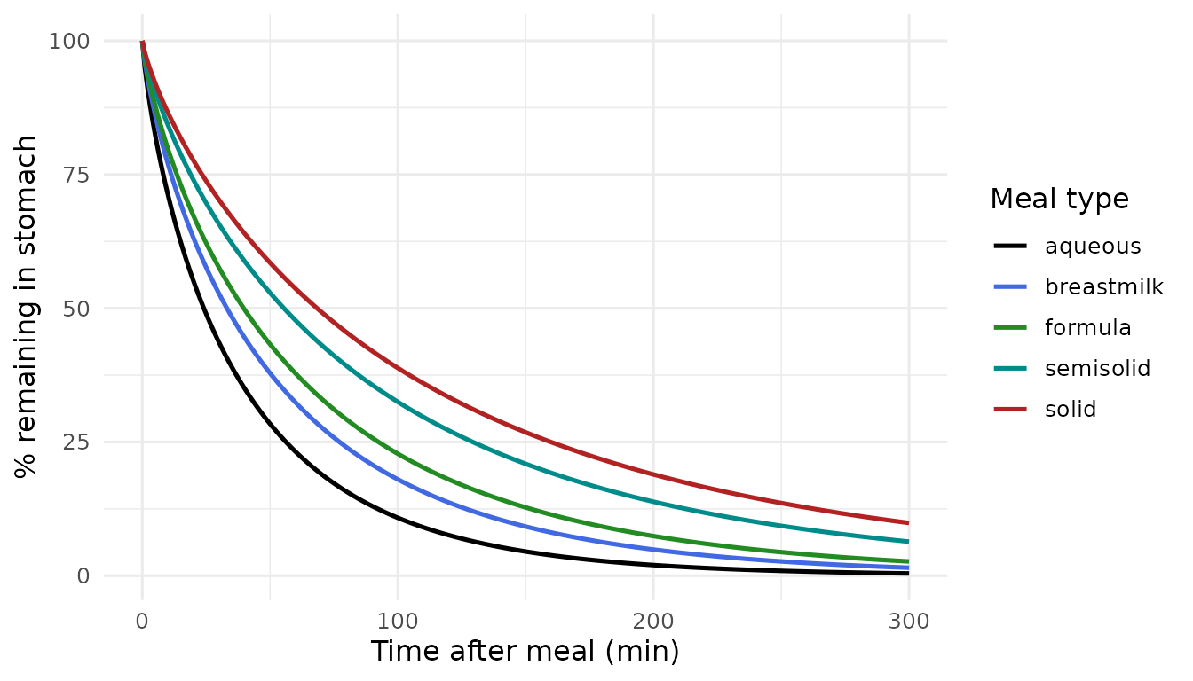
Typical-value gastric-emptying curves by meal type (replicates Bonner 2015 Figure 3 pattern).
Mean gastric residence time comparison
The paper reports typical-value MGRTs from a 1000-individual simulation (Bonner 2015 Results, p. 250). Below the packaged model’s typical-value MGRTs are computed two ways – (i) the AUC-of-percent-remaining divided by 100 (equivalent to Bonner 2015 Eq. 4 for the pure-Weibull mixture at GE(0) = 100), and (ii) the AUMC / AUC as printed in Eq. 4. Both readings land within a few minutes of the paper’s reported meal-type values.
mgrt <- lapply(meals, function(mt) {
  d <- subset(sim_typ, meal == mt)
  auc_pct  <- sum(diff(d$time) * (head(d$gastric_remaining, -1) +
                                  tail(d$gastric_remaining, -1)) / 2)
  aumc_pct <- sum(diff(d$time) * (head(d$time, -1) * head(d$gastric_remaining, -1) +
                                  tail(d$time, -1) * tail(d$gastric_remaining, -1)) / 2)
  data.frame(meal = mt,
             mgrt_auc_min      = auc_pct / 100,
             mgrt_aumc_auc_min = aumc_pct / auc_pct)
})
mgrt <- dplyr::bind_rows(mgrt)
mgrt$paper_reported_min <- c(45, 57, 64, 87, 98)
mgrt <- mgrt |>
  dplyr::rename(
    "Meal type"                            = meal,
    "MGRT AUC/100 (min, simulated)"        = mgrt_auc_min,
    "MGRT AUMC/AUC (min, simulated, Eq.4)" = mgrt_aumc_auc_min,
    "MGRT (min, Bonner 2015 reported)"     = paper_reported_min
  )
knitr::kable(mgrt, digits = 1)| Meal type | MGRT AUC/100 (min, simulated) | MGRT AUMC/AUC (min, simulated, Eq.4) | MGRT (min, Bonner 2015 reported) |
|---|---|---|---|
| aqueous | 41.8 | 50.6 | 45 |
| breastmilk | 56.4 | 64.9 | 57 |
| formula | 66.4 | 73.3 | 64 |
| semisolid | 87.8 | 88.3 | 87 |
| solid | 102.9 | 96.8 | 98 |
The simulated MGRT values track the paper’s rank ordering (aqueous fastest, solid slowest) with a maximum discrepancy of about 6 min on either the AUC or AUMC / AUC reading. Bonner 2015’s reported MGRTs integrate over the paper’s full random-effects distribution (1000 individuals across ages 0.01 - 800 months); the small deviations from the typical-value simulations here are consistent with the nonlinearity of Eq. 4 in PR, which has an omega^2 of 114 (interpreted here as CV% on the logit scale – see Errata) so the population mean and the typical-individual value differ.
Population variability
The paper reports substantial between-study variability, particularly on PR (omega^2 = 114 in Table 3, the largest reported BSV term). Simulating a 200-subject cohort with all IIV terms active illustrates the resulting spread:
set.seed(2015)
sim_pop <- lapply(meals, function(mt) {
  et  <- one_meal_event_table(mt, seq(0, 300, by = 5))
  s   <- rxode2::rxSolve(ui, events = et, nSub = 200)
  d   <- as.data.frame(s)
  d$meal <- mt
  d[, c("meal", "sim.id", "time", "gastric_remaining")]
})
sim_pop <- dplyr::bind_rows(sim_pop)
sim_pop$gastric_remaining <- pmin(pmax(sim_pop$gastric_remaining, 0), 100)
sim_pop_q <- sim_pop |>
  dplyr::group_by(meal, time) |>
  dplyr::summarise(
    q05 = stats::quantile(gastric_remaining, 0.05),
    q50 = stats::quantile(gastric_remaining, 0.50),
    q95 = stats::quantile(gastric_remaining, 0.95),
    .groups = "drop"
  )
ggplot(sim_pop_q, aes(time, q50, colour = meal, fill = meal)) +
  geom_ribbon(aes(ymin = q05, ymax = q95), alpha = 0.15, colour = NA) +
  geom_line(size = 0.9) +
  scale_colour_manual(
    values = c(aqueous = "black", breastmilk = "royalblue",
               formula = "forestgreen", semisolid = "cyan4",
               solid   = "firebrick")
  ) +
  scale_fill_manual(
    values = c(aqueous = "black", breastmilk = "royalblue",
               formula = "forestgreen", semisolid = "cyan4",
               solid   = "firebrick")
  ) +
  labs(x = "Time after meal (min)", y = "% remaining in stomach",
       colour = "Meal type", fill = "Meal type") +
  theme_minimal(base_size = 12)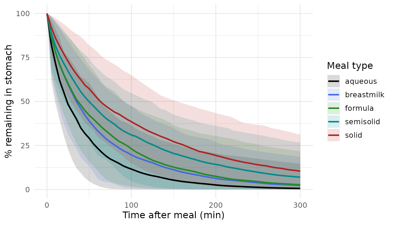
Median (solid) and 5th-95th percentile envelope (ribbon) of % remaining by meal type across 200 simulated subjects.
The envelopes overlap between adjacent meal categories, matching the paper’s Discussion note that individual study-level GE curves are diverse and that the meal-type effect is a study-mean shift rather than a clean between-category separation.
Assumptions and deviations (Errata)
Bonner 2015 is a physiological gastric-emptying meta-analysis with several load-bearing structural details that the paper’s Methods and supplementary material do NOT explicitly resolve, and for which the NONMEM control stream was not available. Each of the three ambiguities below was resolved by a maintainer-approved best-effort choice on 2026-07-24, made with caveats because the missing supplement was not available. All three are listed here so that a downstream user knows what is well-founded and what is a coin toss.
1. Meal-type covariate attachment point
The paper (Methods “Covariate selection and evaluation”, p. 248) states that “the effect of meal type was tested on different parameters of the model shown in Equation (1)”, implying that the authors selected one of the four Eq. 1 parameters (PR, beta1, beta2, gamma1, gamma2 – five options if PR is included) as the attachment point for the five theta_meal coefficients. The paper does NOT state which parameter was selected. This model implements the meal-type theta as a multiplicative scaling on gamma1 (fast-phase Weibull scale) with aqueous as the renormalised reference: gamma1_eff = gamma1 * (theta_meal / theta_Aqueous). Under this choice, the simulated MGRT values in the meal-type comparison table above reproduce the paper’s reported MGRT rank ordering and per-meal-type magnitudes within ~6 min. Alternative attachment points (multiplying gamma2, multiplying both gamma1 and gamma2, modifying beta1 or beta2, or modifying PR) were not implemented; a reader who suspects a different attachment point should re-parameterise from Table 3 accordingly.
2. PR reporting scale
The paper (Methods, p. 247) states that PR was constrained to (0, 100) by a logit transformation, and Table 3 reports “PR (%): 0.26” for the population-typical value. The paper does NOT clarify whether the “0.26” in Table 3 is the back-transformed value on the natural % scale (so PR = 0.26% of the meal remains in the slow phase) or the value on the logit scale (so PR = 100 * expit(0.26) = 56.5% of the meal remains in the slow phase). This model implements the natural-% reading, so llogit_pr = logit(0.26 / 100) = -5.951 with a population-typical PR of 0.26%. Under this reading, the fast-phase term dominates the double Weibull for the typical individual, and PR-driven variability enters primarily through the large omega^2 on llogit_pr.
3. Table 3 “Variability omega^2” unit convention
The paper (Table 3) reports the “Variability omega^2” column with values {114, 38.6, 14.1, 58.7, 19.2} for PR / beta1 / beta2 / gamma1 / gamma2 respectively. The paper does NOT state the unit convention. Three interpretations are plausible:
- Raw log-scale variance (standard NONMEM convention for a log-normal eta model). This gives infeasible BSV – omega^2 = 38.6 on log scale implies a coefficient of variation of ~exp(sqrt(38.6)) ~10^8 %.
- CV%^2 (the reported number IS the coefficient of variation squared). This gives near-zero BSV – omega^2 = 38.6 implies CV = 6.21%.
- CV% (the reported number IS the coefficient of variation as a percentage). This gives plausible-magnitude BSV – omega^2 = 38.6 implies CV = 38.6% -> log-scale variance of log(1 + 0.386^2) = 0.139.
This model implements the CV% reading (interpretation 3), converting each reported value to a log-scale variance via omega^2_log = log(1 + (reported_value / 100)^2). The 200-subject cohort plot above illustrates the resulting between-subject spread, which is qualitatively consistent with the paper’s Figure 4A / 4B scatter of study-level MGRTs.
4. Residual-error N * T weighting (Eq. 3)
Bonner 2015 Eq. 3 encodes the residual error as GE = GE_hat + (theta_w / sqrt(N_ij * T_i)) * epsilon, where N_ij is the number of subjects contributing to time-point ij and T_i is 2 for scintigraphy and 1 for other measurement methods. The N * T weighting is a fit-time construct that nlmixr2’s built-in error models do not natively encode; the packaged model applies theta_w = 11.1 as an unweighted additive residual SD instead. This affects only the residual- error draw magnitude in simulation (not the typical-value trajectory or the MGRT calculations above).
5. Age-covariate exclusion
Bonner 2015 tested postnatal age and gestational age as covariates
after allowance for meal type (Table 2, OFV comparisons). Both were
rejected as non-significant (delta OFV < 0.2 for either age term
added to the meal-type model, versus a required delta of a few points at
alpha = 0.05). Consistent with the paper’s final model, the packaged
extraction does NOT include age effects; PNA and GA are documented in
the model file’s covariatesDataExcluded list so that
downstream users know age was screened and found non-significant.
Postmenstrual age (PMA) was used only for the paper’s graphical
inspection (Figures 4A and 4B) and not as a modelled covariate.
6. Scope reminder
This model is a physiological description of gastric emptying, NOT a
drug PK model. There is no drug, no dose, no plasma compartment; the
sole modelled quantity is the fraction of a test meal remaining in the
stomach at time t. It is intended for use as a
physiological prior when constructing pediatric absorption models (per
Bonner 2015 Discussion, this work is part of a wider Simcyp / Certara
project to inform pediatric oral-absorption PBPK modelling), or as a
standalone descriptor of gastric-emptying-time variability across the
human lifespan. The registry already contains a mechanistic paracetamol
+ gastric-emptying + CCK + gallbladder joint model (Guiastrennec 2016)
that combines a first-order gastric-emptying rate constant with a
drug-PK backbone; users who need a drug-PK-linked gastric-emptying
description in adults should prefer that model.
References
- Bonner JJ, Vajjah P, Abduljalil K, Jamei M, Rostami-Hodjegan A, Tucker GT, Johnson TN (2015). Does age affect gastric emptying time? A model-based meta-analysis of data from premature neonates through to adults. Biopharm Drug Dispos 36(4):245-57. https://doi.org/10.1002/bdd.1937.
- Guiastrennec B et al. (2016). Mechanism-Based Modeling of Gastric Emptying Rate and Gallbladder Emptying in Response to Caloric Intake. CPT Pharmacometrics Syst Pharmacol 5(12):692-700. https://doi.org/10.1002/psp4.12152 (companion drug-PK-linked gastric-emptying model in the nlmixr2lib registry).