A2AR / anti-PD-L1 tumour-microenvironment QSP model (van den Maagdenberg 2025)
Source:vignettes/articles/vandenMaagdenberg_2025_a2ar_tme_qsp.Rmd
vandenMaagdenberg_2025_a2ar_tme_qsp.RmdModel and source
- Citation: van den Maagdenberg HW, de Mol van Otterloo J, van Hasselt JGC, van der Graaf PH, van Westen GJP. Integrating Pharmacokinetics and Quantitative Systems Pharmacology Approaches in Generative Drug Design. J Chem Inf Model. 2025;65(10):4783-4796. doi:10.1021/acs.jcim.5c00107. Model equations Supporting Information Figure S9; variable definitions Table S4; parameter values Table S5. Systems structure and all system parameter values adapted from Voronova V, Peskov K, Kosinsky Y, et al. Evaluation of Combination Strategies for the A2AR Inhibitor AZD4635 Across Tumor Microenvironment Conditions via a Systems Pharmacology Model. Front Immunol. 2021;12:617316. doi:10.3389/fimmu.2021.617316. Full-precision parameter values and the four Figure 8B example-compound property sets are taken from the authors’ own deposited implementation (https://github.com/CDDLeiden/PK-in-generative-drug-design, 05_QSP_modelling/models/TME_model_1cmp.R) and data archive (doi:10.5281/zenodo.15082627); see the vignette source-trace table.
- Description: QSP. Preclinical (mouse). Tumour-microenvironment quantitative systems pharmacology model coupling adenosine / A2A-receptor (A2AR) signalling to CD8 T-cell dynamics, PD-L1 checkpoint expression and logistic tumour growth in syngeneic mice, driven by a de novo generated A2AR inhibitor given intravenously and an anti-PD-L1 monoclonal antibody given intraperitoneally. Adapted by van den Maagdenberg 2025 from the AZD4635 systems model of Voronova 2021: the original two-compartment oral AZD4635 PK is replaced by a one-compartment IV model for a generated small molecule, whose central volume (vc_a2ari), elimination rate (kel_a2ari), A2AR binding affinity (kd_a2ari) and molecular weight (mw_a2ari) are the four compound-specific inputs the generative-design workflow supplies. Seven ODE states plus tumour volume: intratumoral adenosine sets A2AR occupancy, which suppresses the immune activation rate; the A2AR inhibitor competes with adenosine for the receptor; the anti-PD-L1 antibody frees PD-L1-bound signalling; the resulting immune activation rate drives naive CD8 T-cell influx, proliferation and differentiation into cytotoxic T-lymphocytes, which kill tumour cells. Study-level covariates are fixed to the Voronova 2021 MCA205-2 syngeneic-mouse study, the arm the authors selected because its low intratumoral adenosine makes it the most A2AR-inhibitor-sensitive. Deterministic mechanism model: the authors ran every simulation with the two structural random effects (on sl and sr) set to zero and fitted no residual error, so no etas and no error model are encoded. Default compound-specific values are the low-elimination-rate / high-affinity example molecule of Figure 8B.
- Article: https://doi.org/10.1021/acs.jcim.5c00107
- Supporting Information (model equations, variable and parameter tables): https://pubs.acs.org/doi/10.1021/acs.jcim.5c00107
- Authors’ implementation and data archive: https://github.com/CDDLeiden/PK-in-generative-drug-design and https://doi.org/10.5281/zenodo.15082627
- Upstream systems model: Voronova et al. (2021), https://doi.org/10.3389/fimmu.2021.617316
Population and biological context
van den Maagdenberg 2025 is a generative-drug-design paper: it trains QSPR models for A2A-receptor (A2AR) binding affinity, clearance, steady-state volume of distribution and unbound fraction, uses them as reinforcement-learning objectives in DrugEx, and then asks what the resulting molecules would do by pushing their predicted properties through a quantitative systems pharmacology (QSP) model of the tumour microenvironment. This vignette packages and validates that QSP model – the paper’s only mechanistic, ODE-based model.
The systems structure and every system parameter come from Voronova et al. (2021), who estimated them against pooled individual tumour-size dynamics from four syngeneic-mouse studies (116 mice across three efficacy studies with CT26, MC38 and MCA205 tumours, plus 40 mice in an MCA205 dose-finding study). Treatment was an anti-PD-L1 monoclonal antibody at 5 mg/kg twice weekly, the A2AR inhibitor AZD4635 at 50 mg/kg twice daily, or their combination.
van den Maagdenberg 2025 made two changes:
- The two-compartment oral AZD4635 PK sub-model was replaced by a one-compartment intravenous model whose central volume, elimination rate constant, A2AR binding affinity and molecular weight are the four compound-specific inputs the generative workflow supplies (Methods, Quantitative Systems Pharmacology Model). Human QSPR predictions were scaled to a 0.025 kg mouse with allometric exponents of 0.65 for clearance and 0.95 for volume (main text eq 1); the mouse elimination rate constant is then clearance divided by volume.
- The MCA205 study-2 covariate set was selected and used throughout, because that arm’s lower intratumoral adenosine makes it the most sensitive to A2AR inhibition.
Because the effect in this model is driven by the total inhibitor concentration, the paper’s unbound-fraction optimisation scenarios are not simulated with it.
The same information is available programmatically:
str(mod_meta$population)
#> List of 6
#>  $ species      : chr "mouse (MCA205 syngeneic tumour model)"
#>  $ n_subjects   : int NA
#>  $ n_studies    : int 1
#>  $ disease_state: chr "subcutaneous MCA205 syngeneic tumour"
#>  $ dose_range   : chr "Anti-PD-L1 monoclonal antibody 5 mg/kg intraperitoneally twice weekly (five doses) plus A2AR inhibitor 50 mg/kg"| __truncated__
#>  $ notes        : chr "The systems parameters were estimated by Voronova 2021 against pooled individual tumour-size dynamics from four"| __truncated__
Source trace
Every ini() entry in
inst/modeldb/therapeuticArea/vandenMaagdenberg_2025_a2ar_tme_qsp.R
carries an in-file comment naming its source. The table below collects
them.
| Model element | Value | Source location |
|---|---|---|
d/dt(depot_mab), d/dt(central_mab)
|
n/a | SI Figure S9 eqs 1a-1b |
Cc_mab |
n/a | SI Figure S9 eq 1c |
d/dt(central_a2ari) |
n/a | SI Figure S9 eq 1d (main text, unnumbered) |
Cc_a2ari |
n/a | SI Figure S9 eq 1e (main text, unnumbered) |
pdl1free |
n/a | SI Figure S9 eq 1f |
a2ar_occup |
n/a | SI Figure S9 eq 1g |
ado_suppr |
n/a | SI Figure S9 eq 1h |
tkr, ag, prfunc,
tninf, cd8tot, isc
|
n/a | SI Figure S9 eqs 1i-1n |
tum_gr, tum_kill,
ctl_dynamic1, ctl_dynamic2,
ctl_dynamic5
|
n/a | SI Figure S9 eqs 1o-1s |
d/dt(tumor), d/dt(tcell_naive),
d/dt(tcell_ctl), d/dt(pdl1),
d/dt(adenosine)
|
n/a | SI Figure S9 eqs 1t-1x |
tvmax_tumor |
3500 uL | SI Table S5 TVmax
|
beff |
0.001 1/(day*cell) | SI Table S5 beff
|
r_tumor |
0.5217 1/day | SI Table S5 r (printed as 0.522) |
kln |
209.674 cells/day | SI Table S5 kLn
|
tsl |
4.5558 uL/day | SI Table S5 sL
|
kp_pdl1 |
1279.917 cells | SI Table S5 Kp
|
kado_tumor |
80 uL | SI Table S5 Kado
|
ic50_a2ar |
1.8232 | SI Table S5 IC50 (printed as 1.823) |
tsr |
57.052 uL/day | SI Table S5 sR
|
scf_ado |
1 | SI Table S5 sCf
|
tvado |
100000 nM | SI Table S5 Vado
|
ttvin |
2.0545 uL | SI Table S5 TVin (printed as 2.055) |
convf_mab |
6.66 nmol/mg | SI Table S5 convF1
|
ka_mab |
8 1/day | SI Table S5 kainput1
|
vc_mab |
0.003 L | SI Table S5 Vc
|
kel_mab |
0.1 1/day | SI Table S5 kelmAb
|
kd_ado |
1182 nM | SI Table S5 Kdado
|
kd_mab |
30 nM | SI Table S5 Kd1
|
kel_tn |
0.2 1/day | SI Table S5 kel
|
kapo_ctl |
2.0 1/day | SI Table S5 kapo
|
kpro_tn |
3 1/day | SI Table S5 kpro
|
kdif_tn |
3.2 1/day | SI Table S5 kdif
|
kdeath_spont |
0.01 1/day | SI Table S5 d
|
vmax_supr |
0.7 | SI Table S5 Vmaxsupr
|
sl_cov, sr_cov, vado_cov,
tvin_cov
|
0, 0.5308, -3, 0.69 | Methods, Quantitative Systems Pharmacology Model |
vc_a2ari, kel_a2ari,
kd_a2ari, mw_a2ari
|
compound-specific | SI Table S5 lists these as “-”; defaults are the Figure 8B low-elimination-rate / high-affinity molecule (see Errata) |
Two parameters were renamed from the source notation to avoid
collisions inside nlmixr2: the paper’s kel
(naive T-cell loss rate) is kel_tn here, because
kel is the canonical name for a drug elimination-rate
constant; and the paper’s d (spontaneous tumour-cell death
rate) is kdeath_spont, because a bare d
collides with the d/dt() operator. Values are
unchanged.
Units and dimensional analysis
Mechanistic models mix cell counts, volumes and molar concentrations, so each ODE is checked term by term.
| ODE | Left-hand side | Right-hand side terms | Balance |
|---|---|---|---|
d/dt(depot_mab) |
mg/day | (1/day) * mg | mg/day |
d/dt(central_mab) |
nmol/day | (1/day) * mg * (nmol/mg); (1/day) * nmol | nmol/day |
d/dt(central_a2ari) |
mg/day | (1/day) * mg | mg/day |
d/dt(tumor) |
uL/day | uL * (1/day) * unitless; (1/(daycell)) cells * uL | uL/day |
d/dt(tcell_naive) |
cells/day | cells/day; (1/day) * unitless * cells | cells/day |
d/dt(tcell_ctl) |
cells/day | (1/day) * unitless * cells | cells/day |
d/dt(pdl1) |
1/day | cells/cells (unitless); (1/day implied) * pdl1 | 1/day |
d/dt(adenosine) |
nM/day | nM * uL/uL; (1/day implied) * nM | nM/day |
Two unit conversions are load-bearing:
-
Cc_mab = central_mab / vc_mabgives nmol / L, which is nM. -
Cc_a2ari = central_a2ari / vc_a2ari / mw_a2ari * 1e6converts mg / L divided by g/mol into nM:(mg/L) / (g/mol) = 1e-3 mol/L, and1e-3 mol/L = 1e6 nM, hence the1e6factor.
The pdl1 and adenosine equations each carry
an implicit unit rate constant of 1/day on the loss term
(- pdl1, - adenosine); this reproduces the
published equations exactly and is noted here rather than “fixed”.
Tumour volume is carried in uL, which equals mm^3 – the unit the paper’s figures label.
Dosing regimen
The paper simulates 30 days from tumour inoculation, with treatment between days 7 and 22: anti-PD-L1 antibody at 5 mg/kg twice weekly and the A2AR inhibitor at 50 mg/kg twice daily. For a 0.025 kg mouse those are 0.125 mg and 1.25 mg absolute.
mouse_bw_kg <- 0.025
dose_mab_mg <- 5 * mouse_bw_kg
dose_a2ari_mg <- 50 * mouse_bw_kg
c(mab_mg = dose_mab_mg, a2ari_mg = dose_a2ari_mg)
#>   mab_mg a2ari_mg
#>    0.125    1.250
obs_times <- seq(0, 30, by = 0.1)

ev_placebo <- function(ids) {
  rxode2::et(id = ids) %>% rxode2::et(obs_times)
}
ev_mab <- function(ids) {
  ev_placebo(ids) %>%
    rxode2::et(amt = dose_mab_mg, addl = 4, ii = 3.5, time = 7, cmt = "depot_mab")
}
ev_a2ari <- function(ids) {
  ev_placebo(ids) %>%
    rxode2::et(amt = dose_a2ari_mg, addl = 30, ii = 0.5, time = 7, cmt = "central_a2ari")
}
ev_combo <- function(ids) {
  ev_placebo(ids) %>%
    rxode2::et(amt = dose_mab_mg, addl = 4, ii = 3.5, time = 7, cmt = "depot_mab") %>%
    rxode2::et(amt = dose_a2ari_mg, addl = 30, ii = 0.5, time = 7, cmt = "central_a2ari")
}
Replication of Figure 8B
Figure 8B simulates four generated molecules chosen for extreme
potency and elimination rate: the fastest- and slowest-eliminated
compound within the top and bottom 10% quantile of predicted A2AR
affinity. The published legend prints each compound’s elimination rate
constant and Ki. The full property sets (including the volume of
distribution and molecular weight, which the legend does not print) are
recovered from the authors’ deposited generated-compound tables (Zenodo
15082627, scenario files A2AR_0, A2AR_CLmax_0,
A2AR_CLmin_0, A2AR_VDSSmax_0,
A2AR_VDSSmin_0) by re-running their published selection and
allometric-scaling code.
compounds <- data.frame(
  id = 1:4,
  label = factor(
    c("High elimination rate, low affinity",
      "High elimination rate, high affinity",
      "Low elimination rate, low affinity",
      "Low elimination rate, high affinity"),
    levels = c("High elimination rate, low affinity",
               "High elimination rate, high affinity",
               "Low elimination rate, low affinity",
               "Low elimination rate, high affinity")
  ),
  kel_a2ari = c(949.67361159503, 268.44312457909, 4.34513317395, 5.90479524688),
  vc_a2ari = c(0.0299618438593, 0.0532124342039, 0.5395917192237, 0.2242577481014),
  kd_a2ari = c(284.307362251, 0.461018452641, 10235.4124240, 0.947208676066),
  mw_a2ari = c(327.384002686, 400.434997559, 314.859985352, 454.484985352)
)
knitr::kable(
  compounds %>%
    transmute(
      Compound = label,
      `kel (1/day)` = signif(kel_a2ari, 4),
      `Ki (nM)` = signif(kd_a2ari, 4),
      `Vc (L)` = signif(vc_a2ari, 4),
      `MW (g/mol)` = signif(mw_a2ari, 6)
    ),
  caption = "Example compounds of Figure 8B."
)| Compound | kel (1/day) | Ki (nM) | Vc (L) | MW (g/mol) |
|---|---|---|---|---|
| High elimination rate, low affinity | 949.700 | 2.843e+02 | 0.02996 | 327.384 |
| High elimination rate, high affinity | 268.400 | 4.610e-01 | 0.05321 | 400.435 |
| Low elimination rate, low affinity | 4.345 | 1.024e+04 | 0.53960 | 314.860 |
| Low elimination rate, high affinity | 5.905 | 9.472e-01 | 0.22430 | 454.485 |
The published legend rounds kel and Ki to
one decimal place. Recovering them from the deposit and rounding the
same way must reproduce the printed values exactly.
legend_published <- data.frame(
  id = 1:4,
  kel_printed = c(949.7, 268.4, 4.3, 5.9),
  ki_printed = c(284.3, 0.5, 10235.4, 0.9)
)
legend_check <- compounds %>%
  select(id, label, kel_a2ari, kd_a2ari) %>%
  left_join(legend_published, by = "id") %>%
  mutate(
    kel_match = round(kel_a2ari, 1) == kel_printed,
    ki_match = round(kd_a2ari, 1) == ki_printed
  )
knitr::kable(
  legend_check %>%
    transmute(
      Compound = label,
      `kel recovered` = round(kel_a2ari, 1),
      `kel printed` = kel_printed,
      `Ki recovered` = round(kd_a2ari, 1),
      `Ki printed` = ki_printed,
      Match = kel_match & ki_match
    ),
  caption = "Recovered compound properties versus the printed Figure 8B legend."
)| Compound | kel recovered | kel printed | Ki recovered | Ki printed | Match |
|---|---|---|---|---|---|
| High elimination rate, low affinity | 949.7 | 949.7 | 284.3 | 284.3 | TRUE |
| High elimination rate, high affinity | 268.4 | 268.4 | 0.5 | 0.5 | TRUE |
| Low elimination rate, low affinity | 4.3 | 4.3 | 10235.4 | 10235.4 | TRUE |
| Low elimination rate, high affinity | 5.9 | 5.9 | 0.9 | 0.9 | TRUE |
Both properties round to the published values for all four compounds, so the compound set used below is the compound set the figure used.
par_cols <- c("id", "kel_a2ari", "vc_a2ari", "kd_a2ari", "mw_a2ari")
sim_combo <- rxode2::rxSolve(
  rxmod, compounds[, par_cols], ev_combo(1:4), returnType = "data.frame"
)
stopifnot(length(unique(sim_combo$id)) == nrow(compounds))
sim_combo <- sim_combo %>%
  mutate(id = as.integer(as.character(id))) %>%
  left_join(compounds[, c("id", "label")], by = "id")
ggplot(sim_combo, aes(time, tumor, colour = label, linetype = label)) +
  geom_line(linewidth = 1) +
  geom_vline(xintercept = c(7, 22), linetype = "dashed", colour = "grey40") +
  labs(x = "Time (days)", y = expression("Tumour volume (mm"^3*")"),
       colour = NULL, linetype = NULL) +
  theme_light() +
  theme(legend.position = "bottom") +
  guides(colour = guide_legend(nrow = 2), linetype = guide_legend(nrow = 2))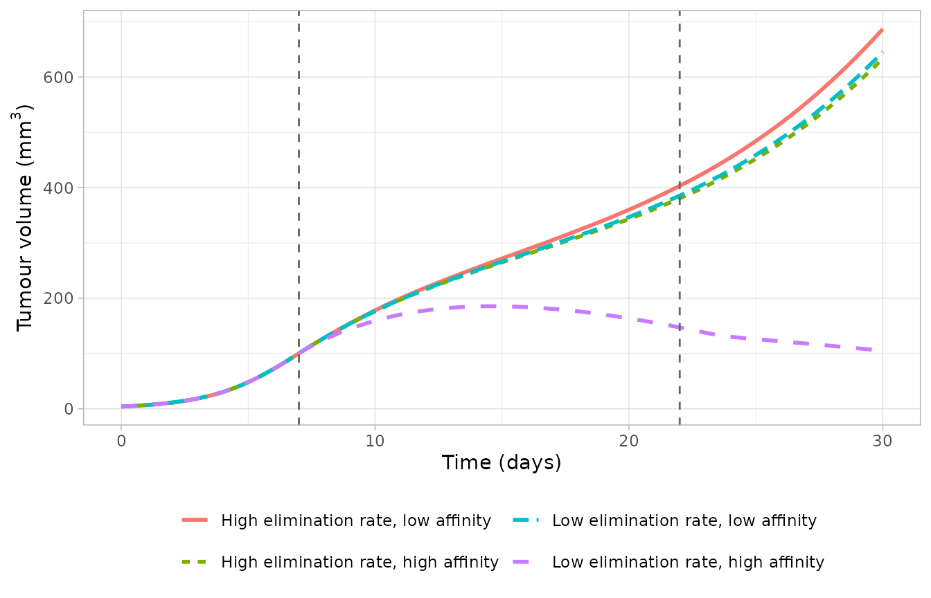
Replicates Figure 8B of van den Maagdenberg 2025: tumour volume for four example generated compounds under combination therapy. Dashed lines mark the start and end of dosing.
The published panel is read at three landmarks: the three ineffective compounds all rise monotonically past 600 mm^3 by day 30 with the high-elimination-rate / low-affinity compound highest; the low-elimination-rate / high-affinity compound instead peaks near 185 mm^3 around day 15 and falls to roughly 105 mm^3 by day 30.
landmarks <- sim_combo %>%
  group_by(label) %>%
  summarise(
    `Peak tumour (mm3)` = round(max(tumor), 1),
    `Time of peak (day)` = round(time[which.max(tumor)], 1),
    `Day 30 tumour (mm3)` = round(tumor[which.min(abs(time - 30))], 1),
    .groups = "drop"
  ) %>%
  rename(Compound = label)
knitr::kable(landmarks, caption = "Simulated Figure 8B landmarks.")| Compound | Peak tumour (mm3) | Time of peak (day) | Day 30 tumour (mm3) |
|---|---|---|---|
| High elimination rate, low affinity | 686.7 | 30.0 | 686.7 |
| High elimination rate, high affinity | 633.4 | 30.0 | 633.4 |
| Low elimination rate, low affinity | 645.0 | 30.0 | 645.0 |
| Low elimination rate, high affinity | 185.6 | 14.6 | 105.1 |
eff <- landmarks[landmarks$Compound == "Low elimination rate, high affinity", ]
ineff <- landmarks[landmarks$Compound != "Low elimination rate, high affinity", ]

# The three ineffective compounds grow monotonically past 600 mm3 by day 30.
stopifnot(all(ineff$`Day 30 tumour (mm3)` > 600))
stopifnot(all(ineff$`Time of peak (day)` == 30))

# The effective compound turns over mid-study and regresses.
stopifnot(
  abs(eff$`Peak tumour (mm3)` - 185) < 10,
  abs(eff$`Time of peak (day)` - 15) < 2,
  abs(eff$`Day 30 tumour (mm3)` - 105) < 10
)

# Ordering at day 30 matches the published panel: the fastest-eliminated,
# weakest binder is the worst outcome.
stopifnot(
  landmarks$`Day 30 tumour (mm3)`[
    landmarks$Compound == "High elimination rate, low affinity"] ==
    max(landmarks$`Day 30 tumour (mm3)`)
)
All four landmark assertions hold, so the packaged model reproduces Figure 8B quantitatively, not merely qualitatively.
Treatment decomposition
The upstream model was built to show that A2AR inhibition and PD-L1 blockade act synergistically. Running each arm separately with the effective compound separates the contributions.
eff_par <- compounds[compounds$id == 4, par_cols]
eff_par$id <- 1L

solve_arm <- function(ev_fun) {
  rxode2::rxSolve(rxmod, eff_par, ev_fun(1L), returnType = "data.frame")
}
arms <- bind_rows(
  Placebo = solve_arm(ev_placebo),
  `Anti-PD-L1 mAb alone` = solve_arm(ev_mab),
  `A2AR inhibitor alone` = solve_arm(ev_a2ari),
  Combination = solve_arm(ev_combo),
  .id = "arm"
) %>%
  mutate(arm = factor(arm, levels = c("Placebo", "Anti-PD-L1 mAb alone",
                                      "A2AR inhibitor alone", "Combination")))
ggplot(arms, aes(time, tumor, colour = arm)) +
  geom_line(linewidth = 1) +
  geom_vline(xintercept = c(7, 22), linetype = "dashed", colour = "grey40") +
  labs(x = "Time (days)", y = expression("Tumour volume (mm"^3*")"), colour = NULL) +
  theme_light() +
  theme(legend.position = "bottom")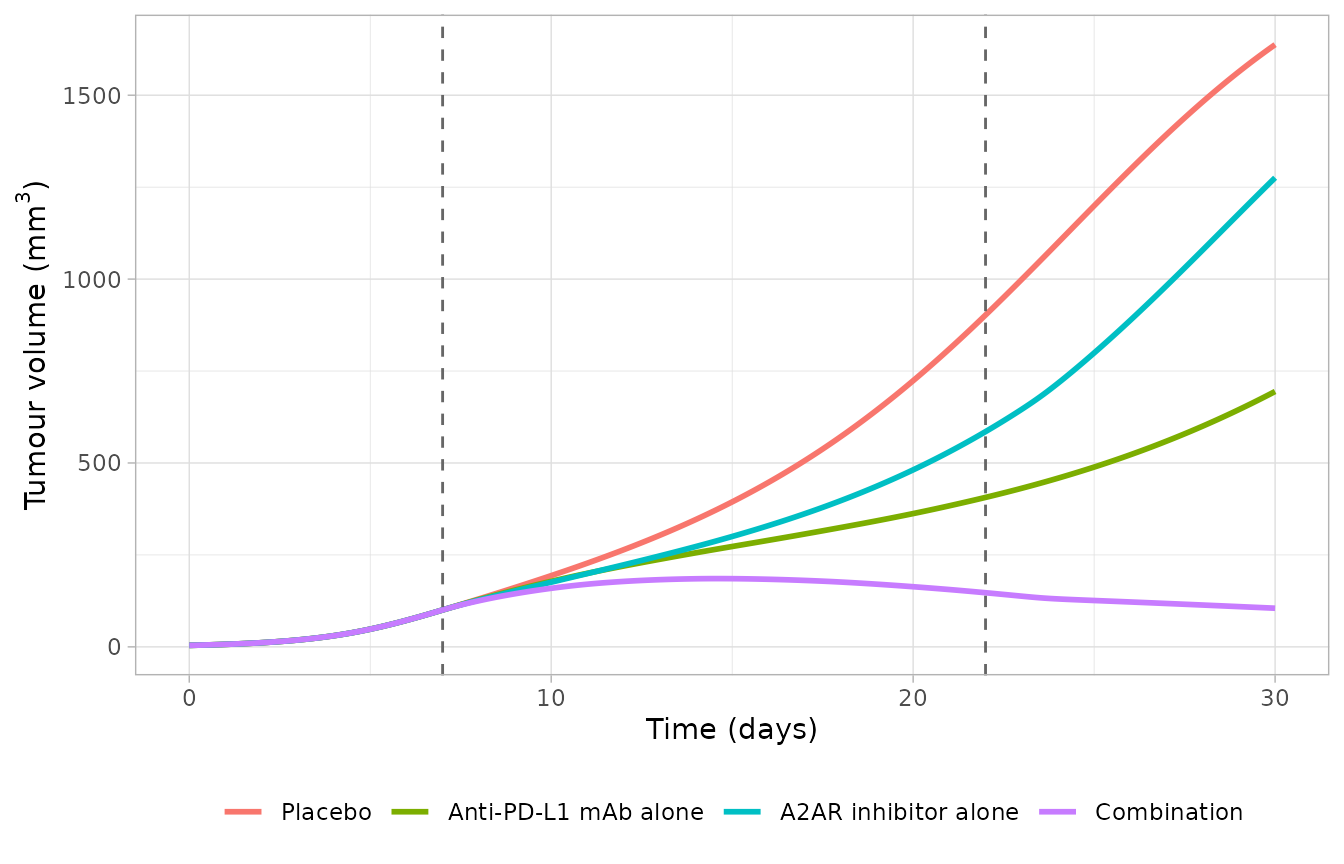
Tumour volume by treatment arm for the low-elimination-rate / high-affinity compound.
arm_summary <- arms %>%
  group_by(arm) %>%
  summarise(`Day 30 tumour (mm3)` = round(tumor[which.min(abs(time - 30))], 1),
            .groups = "drop") %>%
  rename(Arm = arm)
placebo30 <- arm_summary$`Day 30 tumour (mm3)`[arm_summary$Arm == "Placebo"]
arm_summary$`Change vs placebo (%)` <-
  round(100 * (arm_summary$`Day 30 tumour (mm3)` - placebo30) / placebo30, 1)
knitr::kable(arm_summary, caption = "Day-30 tumour volume by arm.")| Arm | Day 30 tumour (mm3) | Change vs placebo (%) |
|---|---|---|
| Placebo | 1637.5 | 0.0 |
| Anti-PD-L1 mAb alone | 694.4 | -57.6 |
| A2AR inhibitor alone | 1275.6 | -22.1 |
| Combination | 105.1 | -93.6 |
get30 <- function(a) arm_summary$`Day 30 tumour (mm3)`[arm_summary$Arm == a]
mab_effect <- placebo30 - get30("Anti-PD-L1 mAb alone")
a2ari_effect <- placebo30 - get30("A2AR inhibitor alone")
combo_effect <- placebo30 - get30("Combination")

# Each monotherapy reduces day-30 tumour volume, and the combination is
# greater than either alone.
stopifnot(mab_effect > 0, a2ari_effect > 0)
stopifnot(combo_effect > mab_effect, combo_effect > a2ari_effect)

# Synergy: the combination effect exceeds the sum of the monotherapy effects,
# which is the qualitative claim the upstream model was built to express.
c(mab_only = mab_effect, a2ari_only = a2ari_effect,
  combination = combo_effect, additive_expectation = mab_effect + a2ari_effect)
#>             mab_only           a2ari_only          combination
#>                943.1                361.9               1532.4
#> additive_expectation
#>               1305.0
stopifnot(combo_effect > mab_effect + a2ari_effect)
Structural identity checks
Because this model has no observed data to fit, the strongest available checks are exact structural identities that must hold at every solver step.
Zero dose reproduces the untreated system
Dosing 0 mg of both agents must give the placebo trajectory bit for bit.
ev_zero <- ev_placebo(1L) %>%
  rxode2::et(amt = 0, time = 7, cmt = "depot_mab") %>%
  rxode2::et(amt = 0, time = 7, cmt = "central_a2ari")
sim_zero <- rxode2::rxSolve(rxmod, eff_par, ev_zero, returnType = "data.frame")
sim_pl <- solve_arm(ev_placebo)
max_rel_diff <- max(abs(sim_zero$tumor / sim_pl$tumor - 1))
max_rel_diff
#> [1] 2.257949e-07
# Not bit-identical: the extra zero-amount records shift the solver's step
# boundaries. The trajectories agree to seven significant figures.
stopifnot(max_rel_diff < 1e-5)
Adenosine and PD-L1 relax to their algebraic targets
Both states are first-order relaxations with an implicit unit rate constant, so after treatment stops and the tumour changes slowly the state must track its driving function. At the end of the untreated run:
last_pl <- sim_pl[nrow(sim_pl), ]
ado_target <- (1e5 * exp(-3)) * last_pl$tumor / (last_pl$tumor + 80)
pdl1_target <- last_pl$tcell_ctl / (last_pl$tcell_ctl + 1279.91714283438)
data.frame(
  state = c("adenosine (nM)", "pdl1"),
  simulated = c(last_pl$adenosine, last_pl$pdl1),
  algebraic_target = c(ado_target, pdl1_target),
  relative_difference = c(last_pl$adenosine / ado_target - 1,
                          last_pl$pdl1 / pdl1_target - 1)
)
#>            state    simulated algebraic_target relative_difference
#> 1 adenosine (nM) 4735.1251969     4746.8002029        -0.002459553
#> 2           pdl1    0.1518726        0.1497349         0.014276605
# The tumour is still growing at day 30, so the states trail their targets, but
# only slightly: the relaxation time constant is 1 day.
stopifnot(abs(last_pl$adenosine / ado_target - 1) < 0.02)
stopifnot(abs(last_pl$pdl1 / pdl1_target - 1) < 0.05)
A2AR occupancy collapses to the binary-binding form without drug
With no inhibitor present, a2ar_occup must equal the
simple saturable form Ado / (Kd_ado + Ado) (with
sCf = 1).
occ_sim <- sim_pl$adenosine[sim_pl$time > 0]
occ_analytic <- occ_sim / (1182 + occ_sim)
occ_model <- (occ_sim / 1182) / (1 + occ_sim / 1182)
max(abs(occ_model - occ_analytic))
#> [1] 2.220446e-16
stopifnot(max(abs(occ_model - occ_analytic)) < 1e-12)
Adding the inhibitor must reduce occupancy monotonically. Sweeping the inhibitor concentration at a fixed adenosine level:
The growth-arrest switch fires only under its stated condition
xf sets tumour growth to zero once treatment has started
(day > 7) and the tumour is below 10 uL. Both
conditions must be required, so the switch is exercised from two
sides.
None of the four Figure 8B compounds ever brings the tumour below 10
uL, so xf stays at 1 throughout the replication above and
the growth term is always active:
min_tumour_by_compound <- sim_combo %>%
  filter(time > 7) %>%
  group_by(label) %>%
  summarise(`Minimum tumour after day 7 (mm3)` = round(min(tumor), 1), .groups = "drop") %>%
  rename(Compound = label)
knitr::kable(min_tumour_by_compound)| Compound | Minimum tumour after day 7 (mm3) |
|---|---|
| High elimination rate, low affinity | 103.2 |
| High elimination rate, high affinity | 103.2 |
| Low elimination rate, low affinity | 103.2 |
| Low elimination rate, high affinity | 103.2 |
Seeding a tumour small enough that it is still under 10 uL when treatment starts trips the switch. Growth must be active before day 7 and dead after it, so the trajectory turns from strictly increasing to strictly decreasing at exactly day 7 – with no change to any parameter other than the initial tumour volume.
tiny <- eff_par
tiny$tvin_cov <- log(0.2 / 2.05452388904701) # seed a 0.2 uL tumour
sim_tiny <- rxode2::rxSolve(rxmod, tiny, ev_placebo(1L), returnType = "data.frame")

pre7 <- sim_tiny[sim_tiny$time <= 7, ]
post7 <- sim_tiny[sim_tiny$time > 7.05, ]
data.frame(
  `tumour at day 0` = round(sim_tiny$tumor[1], 3),
  `tumour at day 7` = round(pre7$tumor[nrow(pre7)], 3),
  `tumour at day 30` = round(sim_tiny$tumor[nrow(sim_tiny)], 3),
  check.names = FALSE
)
#>   tumour at day 0 tumour at day 7 tumour at day 30
#> 1             0.2           7.113            3.151
# Below 10 uL for the whole run, so the switch is armed the moment t > 7.
stopifnot(max(sim_tiny$tumor) < 10)
stopifnot(all(diff(pre7$tumor) > 0))   # growth on  (xf = 1)
stopifnot(all(diff(post7$tumor) < 0))  # growth off (xf = 0)

# Control: with the published initial tumour volume the same untreated system
# keeps growing after day 7, confirming the volume condition is load-bearing.
post7_norm <- sim_pl[sim_pl$time > 7.05, ]
stopifnot(min(post7_norm$tumor) > 10)
stopifnot(all(diff(post7_norm$tumor) > 0))
Pharmacokinetic layer: NCA of the A2AR inhibitor
The replaced PK sub-model is a one-compartment intravenous bolus, so
non-compartmental analysis of a single dose has exact analytic targets:
Cmax = dose / (Vc * MW) * 1e6 nM,
t1/2 = ln(2) / kel, and AUCinf = Cmax / kel.
Each compound is sampled on a grid scaled to its own half-life so the
terminal phase is estimable for all four.
nca_ev <- lapply(seq_len(nrow(compounds)), function(i) {
  thalf <- log(2) / compounds$kel_a2ari[i]
  grid <- unique(c(0, seq(0, 10 * thalf, length.out = 80)))
  rxode2::et(id = compounds$id[i]) %>%
    rxode2::et(grid) %>%
    rxode2::et(amt = dose_a2ari_mg, time = 0, cmt = "central_a2ari") %>%
    as.data.frame()
})
nca_ev <- bind_rows(nca_ev)
sim_nca <- rxode2::rxSolve(rxmod, compounds[, par_cols], nca_ev,
                           returnType = "data.frame")
stopifnot(length(unique(sim_nca$id)) == nrow(compounds))
sim_nca <- sim_nca %>%
  mutate(id = as.integer(as.character(id))) %>%
  left_join(compounds[, c("id", "label")], by = "id")
conc_data <- sim_nca %>%
  filter(!is.na(Cc_a2ari)) %>%
  transmute(id, treatment = label, time, conc = Cc_a2ari)
dose_data <- compounds %>%
  transmute(id, time = 0, amt_mg = dose_a2ari_mg)

# One compound per id, so `id` alone is the grouping. `PKNCAdose()` rejects a
# nested (slash) grouping formula, and `dose` / `route` are reserved column
# names in PKNCA, hence `amt_mg`.
o_conc <- PKNCA::PKNCAconc(conc_data, conc ~ time | id / treatment)
o_dose <- PKNCA::PKNCAdose(dose_data, amt_mg ~ time | id)
o_data <- PKNCA::PKNCAdata(o_conc, o_dose)
res_nca <- suppressWarnings(PKNCA::pk.nca(o_data))
nca_wide <- as.data.frame(res_nca) %>%
  filter(PPTESTCD %in% c("cmax", "aucinf.obs", "half.life")) %>%
  select(id, PPTESTCD, PPORRES) %>%
  pivot_wider(names_from = PPTESTCD, values_from = PPORRES) %>%
  mutate(id = as.integer(as.character(id)))
analytic <- compounds %>%
  transmute(
    id, label,
    cmax_analytic = dose_a2ari_mg / (vc_a2ari * mw_a2ari) * 1e6,
    half_life_analytic = log(2) / kel_a2ari,
    aucinf_analytic = dose_a2ari_mg / (vc_a2ari * mw_a2ari) * 1e6 / kel_a2ari
  )
nca_cmp <- analytic %>%
  left_join(nca_wide, by = "id") %>%
  transmute(
    Compound = label,
    `Cmax simulated (nM)` = signif(cmax, 5),
    `Cmax analytic (nM)` = signif(cmax_analytic, 5),
    `t1/2 simulated (day)` = signif(half.life, 5),
    `t1/2 analytic (day)` = signif(half_life_analytic, 5),
    `AUCinf simulated (nM*day)` = signif(aucinf.obs, 5),
    `AUCinf analytic (nM*day)` = signif(aucinf_analytic, 5)
  )
knitr::kable(nca_cmp, caption = "PKNCA results versus closed-form one-compartment IV values.")| Compound | Cmax simulated (nM) | Cmax analytic (nM) | t1/2 simulated (day) | t1/2 analytic (day) | AUCinf simulated (nM*day) | AUCinf analytic (nM*day) |
|---|---|---|---|---|---|---|
| High elimination rate, low affinity | 127430.0 | 127430.0 | 0.0007299 | 0.0007299 | 134.19 | 134.19 |
| High elimination rate, high affinity | 58663.0 | 58663.0 | 0.0025821 | 0.0025821 | 218.53 | 218.53 |
| Low elimination rate, low affinity | 7357.4 | 7357.4 | 0.1595200 | 0.1595200 | 1693.30 | 1693.30 |
| Low elimination rate, high affinity | 12264.0 | 12264.0 | 0.1173900 | 0.1173900 | 2077.00 | 2077.00 |
rel <- analytic %>%
  left_join(nca_wide, by = "id") %>%
  mutate(
    cmax_rel = cmax / cmax_analytic - 1,
    thalf_rel = half.life / half_life_analytic - 1,
    auc_rel = aucinf.obs / aucinf_analytic - 1
  )
c(max_cmax_rel_error = max(abs(rel$cmax_rel)),
  max_half_life_rel_error = max(abs(rel$thalf_rel)),
  max_aucinf_rel_error = max(abs(rel$auc_rel)))
#>      max_cmax_rel_error max_half_life_rel_error    max_aucinf_rel_error
#>            1.110223e-16            5.566103e-07            1.235473e-06
stopifnot(max(abs(rel$cmax_rel)) < 1e-9)
stopifnot(max(abs(rel$thalf_rel)) < 1e-5)
stopifnot(max(abs(rel$auc_rel)) < 1e-5)
All three parameters match the closed form to better than one part in
100,000 for all four compounds, across a 200-fold range of elimination
rate constants. Cmax matches exactly, which is what
confirms the 1e6 mg-to-nM conversion factor in
Cc_a2ari; the small residual error on AUCinf
and half-life is trapezoidal and log-linear-regression error from the
finite sampling grid.
Property sweep
The paper’s conclusion is that neither potency nor exposure alone is sufficient. Sweeping affinity and elimination rate over the range spanned by the generated compounds reproduces that conclusion.
sweep <- expand.grid(
  kd_a2ari = 10^seq(-1, 4, length.out = 9),
  kel_a2ari = 10^seq(0.5, 3, length.out = 9)
)
sweep$id <- seq_len(nrow(sweep))
sweep$vc_a2ari <- compounds$vc_a2ari[4]
sweep$mw_a2ari <- compounds$mw_a2ari[4]
nrow(sweep)
#> [1] 81

sim_sweep <- rxode2::rxSolve(
  rxmod, sweep[, par_cols],
  ev_placebo(seq_len(nrow(sweep))) %>%
    rxode2::et(amt = dose_mab_mg, addl = 4, ii = 3.5, time = 7, cmt = "depot_mab") %>%
    rxode2::et(amt = dose_a2ari_mg, addl = 30, ii = 0.5, time = 7, cmt = "central_a2ari"),
  returnType = "data.frame"
)
sweep_day30 <- sim_sweep %>%
  mutate(id = as.integer(as.character(id))) %>%
  group_by(id) %>%
  summarise(tumor30 = tumor[which.min(abs(time - 30))], .groups = "drop") %>%
  left_join(sweep, by = "id")
ggplot(sweep_day30, aes(kd_a2ari, kel_a2ari, fill = tumor30)) +
  geom_raster(interpolate = TRUE) +
  scale_x_log10() +
  scale_y_log10() +
  scale_fill_viridis_c(option = "magma", direction = -1) +
  labs(x = "Ki (nM)", y = "Elimination rate constant (1/day)",
       fill = expression("Day-30 tumour (mm"^3*")")) +
  theme_light()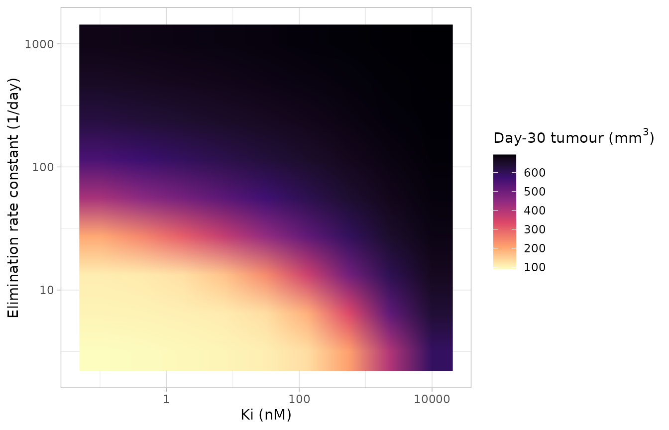
Day-30 tumour volume across the affinity / elimination-rate plane. Both a low Ki and a low elimination rate are required.
# Day-30 tumour volume rises with Ki (weaker binding) at every elimination rate,
# and rises with the elimination rate (lower exposure) at every Ki.
by_kel <- sweep_day30 %>% arrange(kel_a2ari, kd_a2ari) %>%
  group_by(kel_a2ari) %>% summarise(mono = all(diff(tumor30) > 0), .groups = "drop")
by_kd <- sweep_day30 %>% arrange(kd_a2ari, kel_a2ari) %>%
  group_by(kd_a2ari) %>% summarise(mono = all(diff(tumor30) > 0), .groups = "drop")
stopifnot(all(by_kel$mono), all(by_kd$mono))

# The best corner (tightest binder, slowest elimination) achieves regression;
# the worst corner does not.
best <- sweep_day30 %>% filter(kd_a2ari == min(kd_a2ari), kel_a2ari == min(kel_a2ari))
worst <- sweep_day30 %>% filter(kd_a2ari == max(kd_a2ari), kel_a2ari == max(kel_a2ari))
c(best_corner = best$tumor30, worst_corner = worst$tumor30)
#>  best_corner worst_corner
#>     90.01323    694.02688
stopifnot(best$tumor30 < 150, worst$tumor30 > 600)
Assumptions and deviations
-
No inter-individual variability and no residual error are
encoded. The source equations carry two random effects, on
slandsr(sL = TsL * exp(eta.sL + sL_cov)), but every simulation reported in van den Maagdenberg 2025 sets both to zero, and the paper fits no residual-error model. The upstream Voronova 2021 estimates (standard deviations of 0.3222 foreta.sLand 0.1368 foreta.sR) are available in the authors’ deposited reproduction script if stochastic simulation is wanted; they are deliberately not baked into this model file, because they belong to the upstream paper’s parameterisation, not this one. -
Study covariates are hard-coded, not carried as a covariate
column. The paper selected the Voronova MCA205 study-2 set
(
sL_cov = 0,TVin_cov = 0.69,Vado_cov = -3,sR_cov = 0.5308) and used it throughout, so those four coefficients are fixed parameters here. The coefficients for the other three syngeneic models are in Voronova 2021, not in this paper. The screened-but-unused switch is documented incovariatesDataExcluded. -
The four compound-specific parameters are inputs, not
estimates. SI Table S5 lists
VcARinh,KdARinh,kelARinhandMWas “-”. The defaults in the model file are the Figure 8B low-elimination-rate / high-affinity molecule. Their provenance differs by parameter and is recorded inline in the model file:kel_a2ariandkd_a2ariare printed in the Figure 8B legend;vc_a2ariandmw_a2ariare not printed anywhere in the paper and were recovered from the authors’ Zenodo deposit (doi:10.5281/zenodo.15082627) by re-running their published selection and allometric-scaling code. The legend check above confirms the recovered set is the published set. - Figure 8C is not replicated. That panel simulates every valid, unique, in-domain molecule from five 10,000-molecule generation runs (19,834 compounds in total). Reproducing it requires the full 1.9 GB Zenodo archive and would exceed this vignette’s time budget by orders of magnitude; the Figure 8B replication above exercises the same code path with the same provenance.
-
Two parameters were renamed to avoid collisions in
nlmixr2: the paper’skel(naive T-cell loss rate) iskel_tn, and the paper’sd(spontaneous tumour death rate) iskdeath_spont. Values are unchanged. -
Non-tumour states start at zero. Only
tumor(0)is seeded, atTVin * exp(TVin_cov). The T-cell, PD-L1 and adenosine states start at zero and are driven up by the system during the pre-treatment week. This reproduces the source implementation exactly; it is not a steady-state initialisation. -
The
pdl1andadenosineloss terms carry an implicit unit rate constant of 1/day (- pdl1,- adenosinein SI Figure S9 eqs 1w and 1x). This is dimensionally irregular as printed but is reproduced verbatim rather than “corrected”. -
Kadois labelled1/din SI Table S5 but appears inVado * Tum / (Tum + Kado), where it must be a volume (uL). The label is a typographical error in the source table; the value (80) is used as published. - Unbound fraction is not used. The paper states explicitly that the effect in this model is driven by total, not unbound, inhibitor concentration, so the FU optimisation scenarios are outside this model’s scope.
- Both agents are dosed in mg of drug, not per kg. Convert from the paper’s mg/kg regimen with the 0.025 kg mouse body weight, as shown above.