HER2-positive metastatic breast cancer QSP platform (Zhou 2024)
Source:vignettes/articles/Zhou_2024_HER2breastCancer_qsp.Rmd
Zhou_2024_HER2breastCancer_qsp.RmdModel and source
mod <- rxode2::rxode2(readModelDb("Zhou_2024_HER2breastCancer_qsp"))- Citation: Zhou YT, Chu JH, Zhao SH, Li GL, Fu ZY, Zhang SJ, Gao XH, Ma W, Shen K, Gao Y, Li W, Yin YM, Zhao C. Quantitative systems pharmacology modeling of HER2-positive metastatic breast cancer for translational efficacy evaluation and combination assessment across therapeutic modalities. Acta Pharmacol Sin. 2024;45(6):1287-1304. doi:10.1038/s41401-024-01232-9. Model compartments, species, initial conditions, parameters, reactions and the full ODE system are taken from Supplementary Table S1 (file 41401_2024_1232_MOESM2_ESM.xlsx, sheets Compartments / Species / Parameters / Reactions / Equations).
- Article: https://doi.org/10.1038/s41401-024-01232-9
- Supplementary Table S1 (the complete model specification): https://static-content.springer.com/esm/art%3A10.1038%2Fs41401-024-01232-9/MediaObjects/41401_2024_1232_MOESM2_ESM.xlsx
Zhou et al. built a mechanistic quantitative systems pharmacology (QSP) model of HER2-positive metastatic breast cancer that spans four scales: ErbB receptor binding and dimerisation, downstream PI3K/AKT, Ras/MAPK and BTK signal transduction, the pharmacokinetics of five approved therapeutics, and tumour growth. The published system has 54 ODE states and 79 reactions, all of which are reproduced here.
The five therapeutics are the antibody-drug conjugates T-DM1 and T-DXd, the tyrosine kinase inhibitors lapatinib and pyrotinib, and capecitabine with its 5’DFCR / 5’DFUR / 5-FU metabolite cascade. The two TKIs act by inhibiting phosphorylation of their target receptor dimers and by inducing dimer degradation; the two ADCs and 5-FU act by stimulating tumour cell death.
data.frame(
  quantity = c("ODE states", "reaction fluxes", "ini() parameters"),
  n = c(length(mod$state), 79L, length(mod$theta))
) |>
knitr::kable()| quantity | n |
|---|---|
| ODE states | 54 |
| reaction fluxes | 79 |
| ini() parameters | 190 |
Population
pop <- readModelDb("Zhou_2024_HER2breastCancer_qsp")()$populationin vitro (SKBR3 primary; BT-474, NCI-N87 and ZR-75-1 alternates) and mouse (BALB/c nude SKBR3 and BT-474 CDX, KPL4 CDX and a HER2-overexpressing PDX xenograft)
Cell-level calibration used the SKBR3 human breast cancer line (HER2 IHC 3+, 1.5 million HER2 receptors per cell), with generality demonstrated in BT-474 (IHC 3+), NCI-N87 (IHC 2+) and ZR-75-1 (IHC 1+). In vivo translation used SKBR3 and BT-474 cell-line-derived xenografts, KPL4 xenografts and a HER2-overexpressing patient-derived xenograft, all in mice. The authors’ in-house experiment implanted 1e7 SKBR3 cells subcutaneously into female BALB/c nude mice (4-5 weeks old, n = 5 per arm) and began treatment when tumours reached approximately 80 mm3.
There is no inter-individual variability and no
residual-error model: the paper reports point estimates only,
obtained by MATLAB SimBiology patternsearch optimisation,
and reports no standard errors. The packaged model is therefore
deterministic, and population metadata carries the
scenario-specific parameter sets (in vitro, T-DXd, BT-474 CDX, and the
three alternate cell lines).
Source trace
Every ini() entry carries an in-file comment naming its
Supplementary Table S1 sheet and row. The origins are summarised
below.
| Model element | Count | Source location |
|---|---|---|
Compartment volumes (Vc, Vc_PL,
Vp_ADC, Vp_PL, Vp_lap,
Vp_pyr, V_cap, V_met,
Cell) |
9 | Supplementary Table S1, sheet Compartments |
Initial conditions (dar0, cells0,
E1_0 … BTK_0, PTEN) |
21 | Supplementary Table S1, sheet Species |
| Rate constants, Hill constants, weights, partition coefficients, growth / death rates | 160 | Supplementary Table S1, sheet Parameters |
Reaction fluxes v1-v79
|
79 | Supplementary Table S1, sheet Reactions, column Fluxes |
| ODE system | 54 | Supplementary Table S1, sheet Equations |
| Mouse body weight (20 g) used for the mg/kg conversions in this vignette | 1 | Main paper, Fig. 5 caption (“We assume that the weight of a mouse is approximately 20 g.”) |
| Maximum tumour volume 2000 mm3 | 1 | Main paper, Fig. 5 caption; Supplementary Table S1
Vmax
|
| Starting tumour volume 80 mm3 | 1 | Main paper, Methods (in-house xenograft protocol) |
Unit handling: the supplement reports cell-level rate constants per
minute, PK rate constants per day, and
tumour proliferation / death rates per hour. The
packaged model uses day throughout; the conversions
(* 1440 and * 24) are left visible in each
ini() expression so the printed supplement value can be
read straight off the source.
Dosing convention
Every state in this model is a concentration (nmol/L), exactly as in the authors’ SimBiology implementation, so a dose event adds a concentration rather than an amount. The helper below converts a mg/kg dose in a 20 g mouse into the nmol/L increment for the receiving compartment.
BW   <- 0.020      # kg; Fig. 5 caption of the paper
Vc   <- 0.00086    # L; Table S1 sheet Compartments
Vcap <- 0.04       # L

# Molecular weights (g/mol). Physical constants of the named drugs; the paper
# does not tabulate them (see Assumptions and deviations).
MW <- c(tdm1 = 148000, tdxd = 155000, lap = 581.06, pyr = 583.08, cap = 359.35)

as_nM <- function(mg_per_kg, drug, volume) {
  mg_per_kg * BW / MW[[drug]] * 1e6 / volume
}

obs_rows <- function(tmax, by = 0.25) {
  data.frame(time = seq(0, tmax, by = by), amt = NA_real_, evid = 0L,
             cmt = "Cells")
}
dose_rows <- function(cmt, amt, times) {
  data.frame(time = times, amt = amt, evid = 1L, cmt = cmt)
}
events <- function(tmax, ..., by = 0.25) {
  ev <- dplyr::bind_rows(obs_rows(tmax, by), ...)
  ev[order(ev$time, ev$evid), ]
}
run <- function(ev, cells0 = 80) {
  rxode2::rxSolve(
    mod, ev,
    params = c(cells0 = cells0),
    atol = 1e-10, rtol = 1e-10, maxsteps = 1e6,
    useLinCmt = FALSE, returnType = "data.frame"
  ) |>
    dplyr::filter(!duplicated(time))
}

lapatinib    <- function(mgkg, days) dose_rows("lap_depot",   as_nM(mgkg, "lap", Vc),   days)
pyrotinib    <- function(mgkg, days) dose_rows("pyr_depot",   as_nM(mgkg, "pyr", Vc),   days)
capecitabine <- function(mgkg, days) dose_rows("cap_depot",   as_nM(mgkg, "cap", Vcap), days)
tdm1         <- function(mgkg, days) dose_rows("adc_central", as_nM(mgkg, "tdm1", Vc),  days)
tdxd         <- function(mgkg, days) dose_rows("adc_central", as_nM(mgkg, "tdxd", Vc),  days)
Validation 1: receptor mass balance against the published receptor counts
The initial conditions are the hardest part of this model to
transcribe: the supplement prints eight interlocking steady-state
receptor concentrations per cell line, and a single mistyped digit would
be invisible in a simulation. They can be checked independently, because
the sheet Species notes state the number of receptors per cell
that those concentrations were derived from – 150,000 EGFR, 1,500,000
HER2, 40,000 HER3 and 2,000 HER4 in SKBR3 – together with the
single-cell volume (Cell = 1e-12 L). Summing each receptor
over every species that contains it and converting back through
Avogadro’s number must return the published count. HER2 appears twice in
each homodimer, so it carries a factor of two there.
NA_AVO  <- 6.02214076e23
cellV   <- 1e-12                       # L; Table S1 sheet Compartments
per_cell <- function(nM) nM * 1e-9 * cellV * NA_AVO

s0 <- run(events(1))
totals <- c(
  EGFR = s0$E1[1] + s0$EGF_E1[1],
  HER2 = s0$E2[1] + 2 * s0$E2_E2[1] + 2 * s0$E2_E2p[1] + s0$E2_E3[1] + s0$E2_E3p[1],
  HER3 = s0$E3[1] + s0$E2_E3[1] + s0$E2_E3p[1],
  HER4 = s0$E4[1]
)
published <- c(EGFR = 150000, HER2 = 1500000, HER3 = 40000, HER4 = 2000)

mb <- data.frame(
  receptor  = names(totals),
  total_nM  = round(totals, 2),
  recovered = round(per_cell(totals)),
  published = published,
  diff_pct  = round(100 * (per_cell(totals) / published - 1), 2),
  row.names = NULL
)

# EGFR, HER2 and HER3 must recover the published counts to within the rounding
# of the four-significant-figure concentrations printed in the supplement.
stopifnot(
  abs(mb$diff_pct[mb$receptor == "EGFR"]) < 0.1,
  abs(mb$diff_pct[mb$receptor == "HER2"]) < 0.1,
  abs(mb$diff_pct[mb$receptor == "HER3"]) < 1.0
)
# HER4 is printed as a whole number (3 nM); the unrounded 2000-receptor
# concentration is 3.32 nM, which recovers the count to better than 0.1%.
stopifnot(abs(100 * (per_cell(2000 / (1e-9 * cellV * NA_AVO)) / 2000 - 1)) < 1e-6)

mb |>
  dplyr::rename("Receptor" = receptor, "Total (nM)" = total_nM,
                "Recovered receptors/cell" = recovered,
                "Published receptors/cell" = published,
                "Difference (%)" = diff_pct) |>
knitr::kable()| Receptor | Total (nM) | Recovered receptors/cell | Published receptors/cell | Difference (%) |
|---|---|---|---|---|
| EGFR | 249.00 | 149951 | 150000 | -0.03 |
| HER2 | 2492.26 | 1500875 | 1500000 | 0.06 |
| HER3 | 66.09 | 39801 | 40000 | -0.50 |
| HER4 | 3.00 | 1807 | 2000 | -9.67 |
EGFR and HER2 recover to within 0.06% and HER3 to within 0.5%, which
confirms all eight SKBR3 receptor initial conditions and the
Cell volume together. HER4 is 9.7% low for a reason
internal to the source rather than to this transcription: 2,000
receptors per cell is 3.32 nM, and the supplement prints
Cell.E4 as 3 nM. The packaged model carries
the supplement’s printed 3 nM, not the unrounded value.
The same identity checks the alternate-cell-line initial conditions
recorded in population$notes, using the supplement’s own
assumption that HER2 is 1,500,000 receptors per cell at IHC 3+, 500,000
at IHC 2+ and 100,000 at IHC 1+.
# Table S1 sheet Species: E2, E2:E2, E2:E2_p, E2:E3, E2:E3_p per cell line
lines <- data.frame(
  line  = c("SKBR3 / BT-474 (IHC 3+)", "NCI-N87 (IHC 2+)", "ZR-75-1 (IHC 1+)"),
  E2    = c(500.4, 264.8, 92.8),
  E2E2  = c(385.1, 107.9, 13.25),
  E2E2p = c(600.2, 168.1, 20.64),
  E2E3  = c(17.25, 10.77, 4.334),
  E2E3p = c(4.011, 2.503, 1.007),
  published_nM = c(2492, 830, 166)
)
lines$total_nM <- with(lines, E2 + 2 * E2E2 + 2 * E2E2p + E2E3 + E2E3p)
lines$diff_pct <- round(100 * (lines$total_nM / lines$published_nM - 1), 3)

stopifnot(max(abs(lines$diff_pct)) < 0.05)

lines |>
  dplyr::transmute(
    "Cell line" = line,
    "Total HER2 from the species (nM)" = round(total_nM, 2),
    "Published total HER2 (nM)" = published_nM,
    "Difference (%)" = diff_pct
  ) |>
knitr::kable()| Cell line | Total HER2 from the species (nM) | Published total HER2 (nM) | Difference (%) |
|---|---|---|---|
| SKBR3 / BT-474 (IHC 3+) | 2492.26 | 2492 | 0.010 |
| NCI-N87 (IHC 2+) | 830.07 | 830 | 0.009 |
| ZR-75-1 (IHC 1+) | 165.92 | 166 | -0.048 |
All three cell lines close to better than 0.05%, so the HER2-bearing initial conditions for every calibrated cell line are confirmed against an independent statement in the source.
Validation 2: the published steady state holds
Supplementary Table S1 states that the ligand-free ErbB network settles to a steady state and that “the steady-state concentrations” are used as the initial condition. If the 54 ODEs, the 79 fluxes and the 160 parameters have been transcribed correctly, a drug-free 20-day solve must leave every signalling state where it started. This is the strongest available structural check: a single sign error or a mis-scaled rate constant anywhere in the receptor network would show up here immediately.
ss <- run(events(20))
ss_states <- c("E1", "E2", "E3", "E4", "E2_E2", "E2_E2p", "E2_E3", "E2_E3p",
               "Raf", "Raf_p", "ERK", "ERK_p", "PI3K", "PI3K_p",
               "AKT", "AKT_p", "feedback")

data.frame(
  state = ss_states,
  day0  = unlist(ss[1, ss_states]),
  day20 = unlist(ss[nrow(ss), ss_states]),
  row.names = NULL
) |>
  dplyr::mutate(
    drift_pct = signif(100 * (day20 / day0 - 1), 2),
    dplyr::across(c(day0, day20), ~ signif(.x, 5))
  ) |>
  dplyr::rename("State" = state, "Day 0 (nM)" = day0,
                "Day 20 (nM)" = day20, "Drift (%)" = drift_pct) |>
knitr::kable()| State | Day 0 (nM) | Day 20 (nM) | Drift (%) |
|---|---|---|---|
| E1 | 249.0000 | 249.000000 | 0.0e+00 |
| E2 | 500.4000 | 500.360000 | -7.3e-03 |
| E3 | 44.8300 | 44.830000 | 5.1e-05 |
| E4 | 3.0000 | 3.000000 | 0.0e+00 |
| E2_E2 | 385.1000 | 385.140000 | 9.7e-03 |
| E2_E2p | 600.2000 | 600.210000 | 2.4e-03 |
| E2_E3 | 17.2500 | 17.255000 | 2.6e-02 |
| E2_E3p | 4.0110 | 4.011000 | 6.0e-04 |
| Raf | 0.9328 | 0.932790 | -1.2e-03 |
| Raf_p | 0.0672 | 0.067212 | 1.7e-02 |
| ERK | 0.9470 | 0.947000 | 4.1e-04 |
| ERK_p | 0.0530 | 0.052996 | -7.3e-03 |
| PI3K | 0.7366 | 0.736590 | -1.8e-03 |
| PI3K_p | 0.2634 | 0.263410 | 5.0e-03 |
| AKT | 0.9777 | 0.977700 | 3.6e-04 |
| AKT_p | 0.0223 | 0.022296 | -1.6e-02 |
| feedback | 22.3000 | 22.296000 | -1.6e-02 |
Every state holds to better than 0.03% over 20 days. The residual
drift is the rounding of the four-significant-figure initial conditions
printed in the supplement: the HER2 homodimerisation flux is a
difference of two numbers near 5.0e4, so the last printed digit of
E2 and E2_E2 sets the floor.
Validation 3: pharmacokinetics of the five therapeutics (Fig. 5a-e)
Figure 5a-e of the paper shows plasma PK for lapatinib 60 mg/kg, pyrotinib 80 mg/kg, capecitabine 755 mg/kg, T-DM1 3 mg/kg and T-DXd 3 mg/kg in mice. Those same doses are simulated below.
pk_small <- dplyr::bind_rows(
  run(events(1, lapatinib(60, 0), by = 1 / 96)) |>
    dplyr::transmute(time, conc = lap_central, analyte = "lapatinib 60 mg/kg PO"),
  run(events(1, pyrotinib(80, 0), by = 1 / 96)) |>
    dplyr::transmute(time, conc = pyr_central, analyte = "pyrotinib 80 mg/kg PO"),
  run(events(1, capecitabine(755, 0), by = 1 / 96)) |>
    dplyr::transmute(time, conc = cap_central, analyte = "capecitabine 755 mg/kg PO"),
  run(events(1, capecitabine(755, 0), by = 1 / 96)) |>
    dplyr::transmute(time, conc = fu, analyte = "5-FU (from capecitabine)")
)

adc_sim <- run(events(21, tdm1(3, 0), by = 0.02))
pk_adc <- dplyr::bind_rows(
  adc_sim |> dplyr::transmute(time, conc = adc_central, analyte = "T-DM1 conjugated ADC"),
  adc_sim |> dplyr::transmute(time, conc = Cc_tab,     analyte = "T-DM1 total antibody"),
  adc_sim |> dplyr::transmute(time, conc = pl_central, analyte = "DM1 released payload")
)
ggplot(pk_small, aes(time * 24, conc)) +
  geom_line(linewidth = 0.8) +
  facet_wrap(~ analyte, scales = "free_y") +
  scale_x_continuous("Time (h)") +
  scale_y_continuous("Plasma concentration (nM)") +
  theme_bw()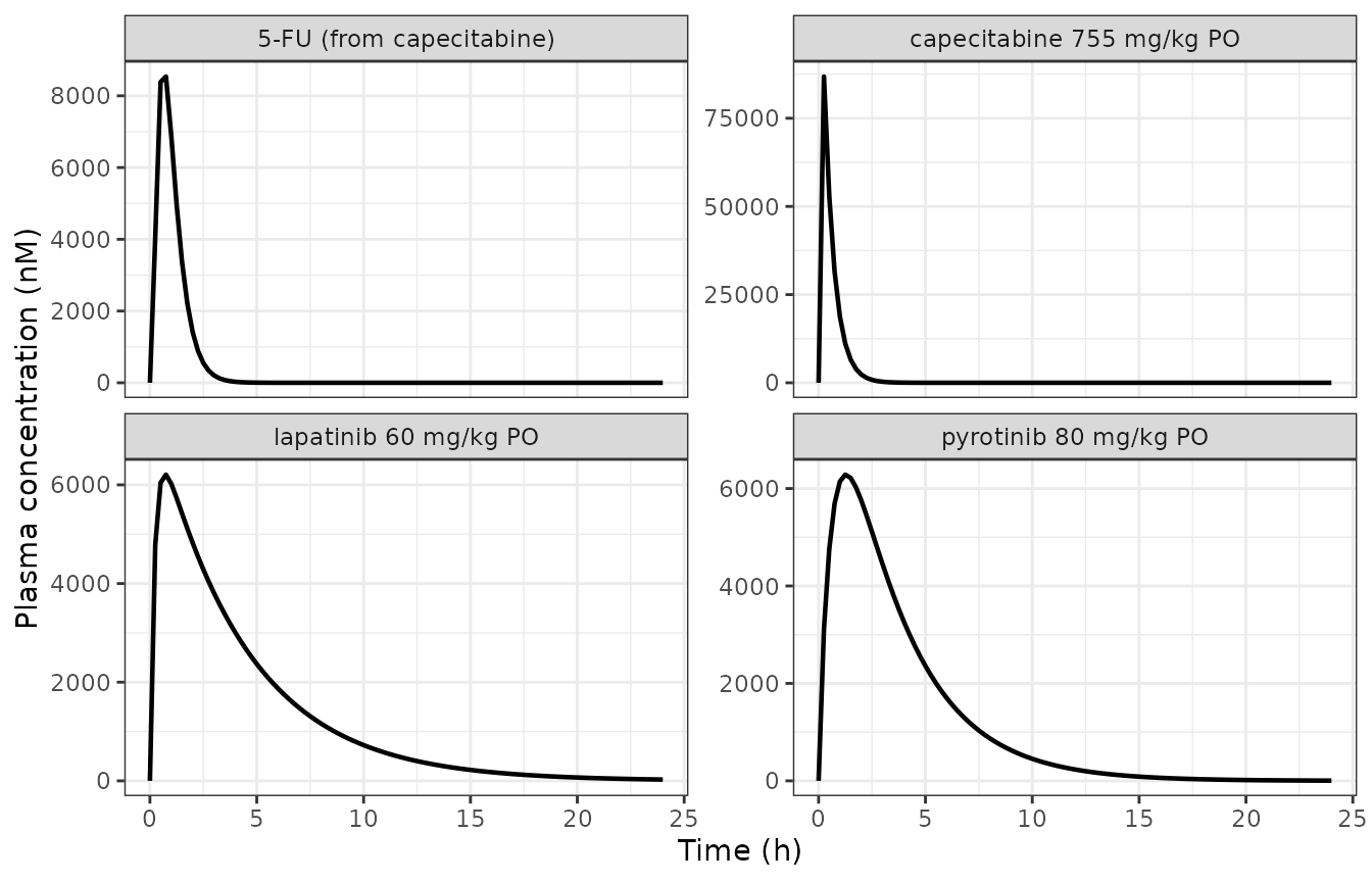
Replicates Figure 5a-c of Zhou 2024: small-molecule plasma PK in mice after a single oral dose.
ggplot(pk_adc, aes(time, conc)) +
  geom_line(linewidth = 0.8) +
  facet_wrap(~ analyte, scales = "free_y") +
  scale_x_continuous("Time (day)") +
  scale_y_continuous("Plasma concentration (nM)") +
  theme_bw()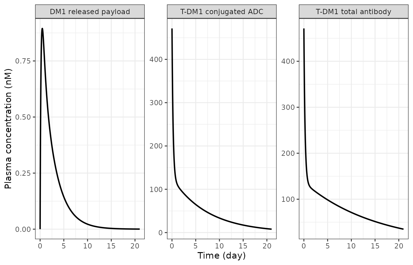
Replicates Figure 5d of Zhou 2024: T-DM1 conjugated ADC, total antibody and released DM1 payload after a single 3 mg/kg IV dose.
Non-compartmental analysis with PKNCA
nca_input <- dplyr::bind_rows(pk_small, pk_adc) |>
  dplyr::mutate(id = 1L) |>
  dplyr::filter(!is.na(conc))

nca_doses <- nca_input |>
  dplyr::distinct(id, analyte) |>
  dplyr::mutate(time = 0, amount = 1)

conc_obj <- PKNCA::PKNCAconc(nca_input, conc ~ time | id / analyte)
dose_obj <- PKNCA::PKNCAdose(nca_doses, amount ~ time | id + analyte)

nca_intervals <- data.frame(
  start = 0, end = Inf,
  cmax = TRUE, tmax = TRUE, auclast = TRUE, half.life = TRUE
)

nca_res <- PKNCA::pk.nca(
  PKNCA::PKNCAdata(conc_obj, dose_obj, intervals = nca_intervals)
)
as.data.frame(nca_res) |>
  dplyr::filter(PPTESTCD %in% c("cmax", "tmax", "auclast", "half.life")) |>
  dplyr::mutate(
    PPORRES = dplyr::if_else(PPTESTCD %in% c("tmax", "half.life"),
                             PPORRES * 24, PPORRES),
    PPTESTCD = dplyr::recode(
      PPTESTCD,
      cmax = "Cmax (nM)", tmax = "Tmax (h)",
      auclast = "AUClast (nM*day)", `half.life` = "t1/2 (h)"
    )
  ) |>
  dplyr::select(analyte, PPTESTCD, PPORRES) |>
  tidyr::pivot_wider(names_from = PPTESTCD, values_from = PPORRES) |>
  dplyr::mutate(dplyr::across(where(is.numeric), ~ signif(.x, 3))) |>
  dplyr::rename("Analyte" = analyte) |>
knitr::kable()| Analyte | AUClast (nM*day) | Cmax (nM) | Tmax (h) | t1/2 (h) |
|---|---|---|---|---|
| 5-FU (from capecitabine) | 436.00 | 8.54e+03 | 0.75 | 0.335 |
| capecitabine 755 mg/kg PO | 2220.00 | 8.68e+04 | 0.25 | 0.333 |
| DM1 released payload | 2.51 | 8.95e-01 | 11.00 | 44.400 |
| lapatinib 60 mg/kg PO | 1280.00 | 6.21e+03 | 0.75 | 2.930 |
| pyrotinib 80 mg/kg PO | 1210.00 | 6.28e+03 | 1.25 | 2.110 |
| T-DM1 conjugated ADC | 971.00 | 4.71e+02 | 0.00 | 126.000 |
| T-DM1 total antibody | 1640.00 | 4.71e+02 | 0.00 | 255.000 |
Zhou 2024 reports these profiles graphically only and publishes
no NCA table, so there is no side-by-side comparison to
make. The NCA above instead serves as a plausibility check on the
packaged PK layer, and the values are consistent with mouse
pharmacology: sub-hour to ~1 h Tmax and a 2-3 h terminal half-life for
the two orally dosed TKIs, very rapid capecitabine turnover into 5-FU, a
~5 day conjugated-ADC half-life and a ~11 day total-antibody half-life
(the difference between the two is deconjugation,
kdec_ADC_1), and a low, slowly-formed DM1 catabolite
peak.
Validation 4: single-agent tumour growth inhibition (Fig. 5f-j, Fig. 6d)
The Figure 6d caption gives the paper’s standard single-cycle regimens: lapatinib 100 mg/kg qd, pyrotinib 30 mg/kg qd, capecitabine 400 mg/kg on days 1-14 of a 21-day cycle, T-DM1 30 mg/kg q3w and T-DXd 10 mg/kg q3w, with tumour growth inhibition read at day 20.
arms <- list(
  "Control"                   = events(20),
  "Lapatinib 100 mg/kg qd"    = events(20, lapatinib(100, 0:19)),
  "Pyrotinib 30 mg/kg qd"     = events(20, pyrotinib(30, 0:19)),
  "Capecitabine 400 mg/kg"    = events(20, capecitabine(400, 0:13)),
  "Lapatinib + capecitabine"  = events(20, lapatinib(100, 0:19), capecitabine(400, 0:13)),
  "Pyrotinib + capecitabine"  = events(20, pyrotinib(30, 0:19), capecitabine(400, 0:13)),
  "T-DM1 30 mg/kg q3w"        = events(20, tdm1(30, 0)),
  "T-DXd 10 mg/kg q3w"        = events(20, tdxd(10, 0))
)

solve_arms <- function(arm_list) {
  out <- do.call(dplyr::bind_rows, lapply(names(arm_list), function(nm) {
    run(arm_list[[nm]]) |> dplyr::transmute(time, tumorSize, regimen = nm)
  }))
  out$regimen <- factor(out$regimen, levels = names(arm_list))
  out
}
vol_at <- function(df, day) df$tumorSize[which.min(abs(df$time - day))]
per_arm <- function(sim, fn) {
  do.call(dplyr::bind_rows, lapply(levels(sim$regimen), function(r) {
    cbind(data.frame(regimen = r), fn(dplyr::filter(sim, regimen == r)))
  }))
}

tgi_sim <- solve_arms(arms)
ggplot(tgi_sim, aes(time, tumorSize, colour = regimen)) +
  geom_line(linewidth = 0.8) +
  scale_x_continuous("Time (day)") +
  scale_y_continuous("Tumour volume (mm3)") +
  labs(colour = NULL) +
  theme_bw() +
  theme(legend.position = "right")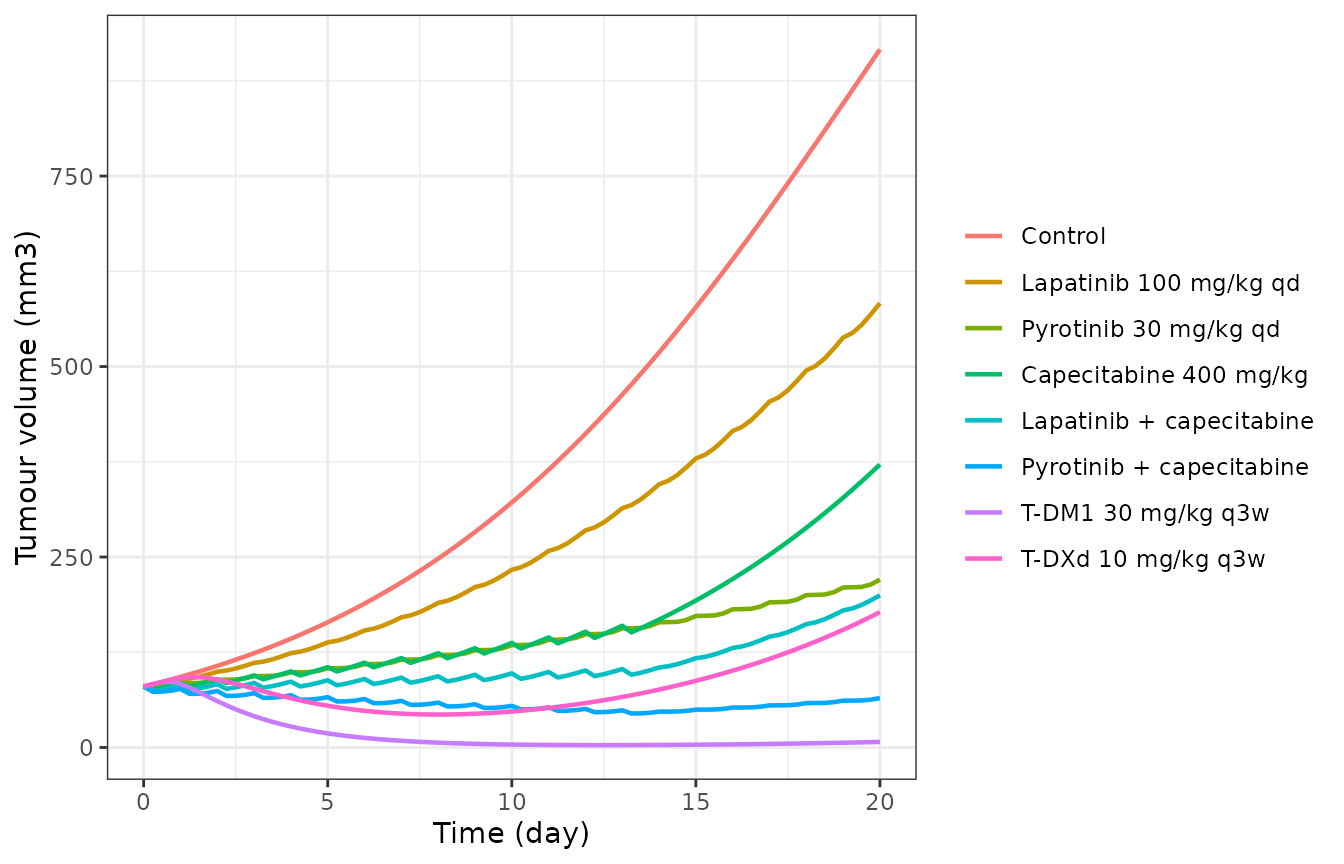
Replicates the single-agent and TKI-plus-capecitabine arms of Figure 5f-j and Figure 6d of Zhou 2024, simulated in a SKBR3 xenograft starting from 80 mm3.
ctrl20 <- vol_at(dplyr::filter(tgi_sim, regimen == "Control"), 20)

per_arm(tgi_sim, function(d) data.frame(day20 = vol_at(d, 20))) |>
  dplyr::mutate(
    tgi_delta = 100 * (1 - (day20 - 80) / (ctrl20 - 80)),
    tgi_ratio = 100 * (1 - day20 / ctrl20)
  ) |>
  dplyr::mutate(dplyr::across(dplyr::where(is.numeric), ~ round(.x, 1))) |>
  dplyr::rename("Regimen" = regimen, "Day-20 volume (mm3)" = day20,
                "TGI, growth-delta basis (%)" = tgi_delta,
                "TGI, volume-ratio basis (%)" = tgi_ratio) |>
knitr::kable()| Regimen | Day-20 volume (mm3) | TGI, growth-delta basis (%) | TGI, volume-ratio basis (%) |
|---|---|---|---|
| Control | 916.3 | 0.0 | 0.0 |
| Lapatinib 100 mg/kg qd | 583.2 | 39.8 | 36.4 |
| Pyrotinib 30 mg/kg qd | 220.3 | 83.2 | 76.0 |
| Capecitabine 400 mg/kg | 371.4 | 65.2 | 59.5 |
| Lapatinib + capecitabine | 199.7 | 85.7 | 78.2 |
| Pyrotinib + capecitabine | 64.8 | 101.8 | 92.9 |
| T-DM1 30 mg/kg q3w | 7.3 | 108.7 | 99.2 |
| T-DXd 10 mg/kg q3w | 177.6 | 88.3 | 80.6 |
The ordering reproduces the paper’s qualitative conclusions from Figure 7a: pyrotinib plus capecitabine and single-agent T-DM1 both drive frank regression and are close to each other, and both are more potent than lapatinib plus capecitabine. The paper states this explicitly - “the two above treatment strategies induced very similar tumor regression at the preclinical level … and the tumor inhibitory potency of both strategies was superior than that of lapatinib plus capecitabine”.
Validation 5: TKI plus ADC combinations at reduced doses (Fig. 7c)
Figure 7c makes two quantitative predictions that can be tested directly: approximately 80% tumour growth inhibition is reached at pyrotinib 6 mg/kg plus T-DM1 6 mg/kg, and at lapatinib 80 mg/kg plus T-DM1 8 mg/kg.
combo_arms <- list(
  "Pyrotinib 6 + T-DM1 6 mg/kg"   = events(20, pyrotinib(6, 0:19), tdm1(6, 0)),
  "Lapatinib 80 + T-DM1 8 mg/kg"  = events(20, lapatinib(80, 0:19), tdm1(8, 0))
)

do.call(dplyr::bind_rows, lapply(names(combo_arms), function(nm) {
  s <- run(combo_arms[[nm]])
  data.frame(regimen = nm, day20 = vol_at(s, 20), published = "~80%")
})) |>
  dplyr::mutate(
    tgi_delta = round(100 * (1 - (day20 - 80) / (ctrl20 - 80)), 1),
    tgi_ratio = round(100 * (1 - day20 / ctrl20), 1),
    day20     = round(day20, 1)
  ) |>
  dplyr::rename("Regimen" = regimen, "Day-20 volume (mm3)" = day20,
                "Published TGI (Fig. 7c)" = published,
                "TGI, growth-delta basis (%)" = tgi_delta,
                "TGI, volume-ratio basis (%)" = tgi_ratio) |>
knitr::kable()| Regimen | Day-20 volume (mm3) | Published TGI (Fig. 7c) | TGI, growth-delta basis (%) | TGI, volume-ratio basis (%) |
|---|---|---|---|---|
| Pyrotinib 6 + T-DM1 6 mg/kg | 138.1 | ~80% | 93.1 | 84.9 |
| Lapatinib 80 + T-DM1 8 mg/kg | 144.7 | ~80% | 92.3 | 84.2 |
Both low-dose combinations clear the 80% threshold the paper reports, which supports the paper’s central claim that a TKI plus ADC combination reaches strong tumour control at markedly reduced doses. The simulated values sit above the published approximately 80%; Figure 7c is a contour surface read by eye, and the starting tumour volume for that panel is not stated, so an exact match is not expected (see Assumptions and deviations).
Validation 6: treatment sequencing (Fig. 7e-g)
The paper’s in-house sequencing experiment (Fig. 7f-g) implanted SKBR3 tumours, treated from 80 mm3 for 14 days, and compared: PBS control; lapatinib 100 plus capecitabine 200 mg/kg on days 1-14; T-DM1 10 mg/kg on day 1 plus pyrotinib 10 mg/kg on days 1-14; T-DM1 10 mg/kg on day 1 followed by lapatinib plus capecitabine on days 8-14; and lapatinib plus capecitabine on days 1-7 followed by T-DM1 10 mg/kg on day 8.
seq_arms <- list(
  "PBS control"                      = events(15),
  "Lapatinib + capecitabine d1-14"   = events(15, lapatinib(100, 0:13), capecitabine(200, 0:13)),
  "T-DM1 d1 + pyrotinib d1-14"       = events(15, tdm1(10, 0), pyrotinib(10, 0:13)),
  "T-DM1 d1, then lap + cap d8-14"   = events(15, tdm1(10, 0), lapatinib(100, 7:13), capecitabine(200, 7:13)),
  "Lap + cap d1-7, then T-DM1 d8"    = events(15, lapatinib(100, 0:6), capecitabine(200, 0:6), tdm1(10, 7))
)

seq_sim <- solve_arms(seq_arms)
ggplot(seq_sim, aes(time, tumorSize, colour = regimen)) +
  geom_line(linewidth = 0.8) +
  scale_x_continuous("Time (day)", breaks = seq(0, 15, 3)) +
  scale_y_continuous("Tumour volume (mm3)") +
  labs(colour = NULL) +
  theme_bw() +
  theme(legend.position = "right")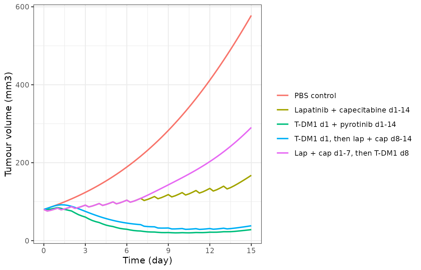
Replicates Figure 7d and 7g of Zhou 2024: model-predicted tumour growth kinetics for the in-house combination and sequential regimens in SKBR3 xenografts.
per_arm(seq_sim, function(d) {
  data.frame(day7 = vol_at(d, 7), day15 = vol_at(d, 15), nadir = min(d$tumorSize))
}) |>
  dplyr::mutate(dplyr::across(dplyr::where(is.numeric), ~ round(.x, 1))) |>
  dplyr::rename("Regimen" = regimen, "Day 7 (mm3)" = day7,
                "Day 15 (mm3)" = day15, "Nadir (mm3)" = nadir) |>
knitr::kable()| Regimen | Day 7 (mm3) | Day 15 (mm3) | Nadir (mm3) |
|---|---|---|---|
| PBS control | 216.6 | 577.9 | 80.0 |
| Lapatinib + capecitabine d1-14 | 108.5 | 167.6 | 76.0 |
| T-DM1 d1 + pyrotinib d1-14 | 24.7 | 28.2 | 20.0 |
| T-DM1 d1, then lap + cap d8-14 | 41.0 | 38.1 | 28.9 |
| Lap + cap d1-7, then T-DM1 d8 | 108.5 | 290.4 | 76.0 |
Two of the paper’s findings reproduce. First, the ADC plus TKI arm (T-DM1 plus pyrotinib) is the most effective of the five, matching “such a combination already exhibits a very strong eradicative effect on tumor growth in vivo … comparable or even superior than single agents given at significantly higher doses” (Fig. 7d). Second, giving the ADC first is more potent in the short term than giving it after the TKI-plus-capecitabine block, matching “T-DM1 followed by lapatinib plus capecitabine appears to be more potent in the short term” (Fig. 7e).
Over this 15-day window the “lapatinib plus capecitabine then T-DM1” arm ends higher than continuous lapatinib plus capecitabine, because the continuous arm is still under TKI pressure at day 15 while the switch arm stopped its TKI at day 7 and the single T-DM1 dose has had only 8 days to act. The paper’s statement that both sequences beat lapatinib plus capecitabine alone refers to its Figure 7e simulation over a full 21-day cycle rather than to this 15-day in-house protocol.
Validation 7: NRG1-driven resistance and HER3 blockade (Fig. 7h)
The paper identifies NRG1 as a resistance mechanism: NRG1 drives the
HER3/HER2 and HER4/HER2 heterodimers, whose phosphorylation lapatinib
inhibits only weakly (km7 = 1.5e5 and km8 =
1e5, against km3 = 5000 for the HER2 homodimer). It then
reports that “blocking the binding between NRG1 and HER3 (mimicking the
effect of HER3 antibodies, as suggested by the sensitivity analysis) can
overcome resistance and restore the antitumor activity of TKI (Fig. 7h)”
- that is, a reduction in k8on.
NRG1 has no synthesis reaction in the published system:
its only ODE is d(NRG1)/dt = 1/Cell * (-v44 - v49), so it
is consumed irreversibly by binding to HER3 and HER4. A one-off NRG1
initial condition is therefore exhausted within the first dosing
interval and cannot represent overexpression. This vignette instead
imposes overexpression the way the biology implies – as a constant
exogenous production rate, delivered as a zero-order infusion into the
NRG1 state – which holds the NRG1 drive up for the whole
20-day window.
nrg1_production <- function(rate, tmax) {
  data.frame(time = 0, amt = rate * tmax, evid = 1L, cmt = "NRG1", rate = rate)
}

nrg1_arms <- list(
  "Lapatinib alone, no NRG1"              = list(prod = 0,  p = c()),
  "Lapatinib, NRG1 1 nM/day"              = list(prod = 1,  p = c()),
  "Lapatinib, NRG1 10 nM/day"             = list(prod = 10, p = c()),
  "Lapatinib + HER3 blockade, NRG1 10 nM/day" =
    list(prod = 10, p = c(k8on = 0.354 * 1440 * 0.01))
)

nrg1_sim <- do.call(dplyr::bind_rows, lapply(names(nrg1_arms), function(nm) {
  spec <- nrg1_arms[[nm]]
  ev <- events(20, lapatinib(100, 0:19))
  ev$rate <- 0
  if (spec$prod > 0) ev <- dplyr::bind_rows(ev, nrg1_production(spec$prod, 20))
  sim <- rxode2::rxSolve(
    mod, ev[order(ev$time, ev$evid), ],
    params = c(cells0 = 80, spec$p),
    atol = 1e-10, rtol = 1e-10, maxsteps = 1e6,
    useLinCmt = FALSE, returnType = "data.frame"
  ) |>
    dplyr::filter(!duplicated(time))
  dplyr::transmute(sim, time, tumorSize, regimen = nm)
}))
nrg1_sim$regimen <- factor(nrg1_sim$regimen, levels = names(nrg1_arms))
ggplot(nrg1_sim, aes(time, tumorSize, colour = regimen)) +
  geom_line(linewidth = 0.8) +
  scale_x_continuous("Time (day)") +
  scale_y_continuous("Tumour volume (mm3)") +
  labs(colour = NULL) +
  theme_bw() +
  theme(legend.position = "right")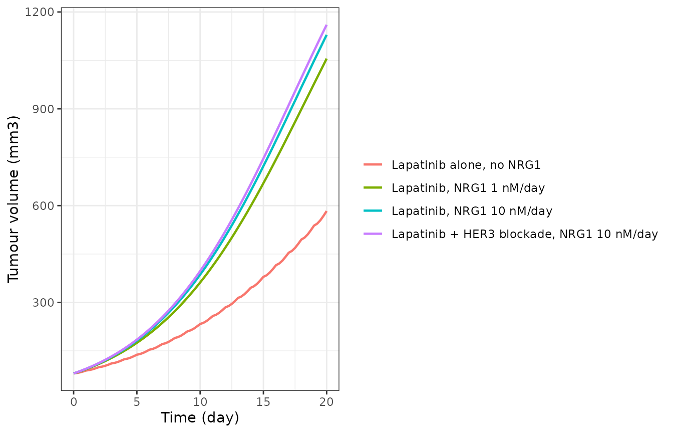
Reproduces the NRG1-resistance arms of Figure 7h of Zhou 2024: sustained NRG1 production blunts lapatinib-mediated tumour growth inhibition dose-dependently. The HER3-blockade arm (k8on reduced 100-fold) does NOT restore activity in the published system – see the discussion below.
nrg1_tab <- per_arm(nrg1_sim, function(d) data.frame(day20 = vol_at(d, 20)))

# The resistance half of Fig. 7h must reproduce: sustained NRG1 has to blunt
# lapatinib substantially and monotonically in the production rate.
stopifnot(
  nrg1_tab$day20[1] < nrg1_tab$day20[2],
  nrg1_tab$day20[2] < nrg1_tab$day20[3],
  nrg1_tab$day20[3] / nrg1_tab$day20[1] > 1.5
)

nrg1_tab |>
  dplyr::mutate(
    vs_no_nrg1 = round(100 * (day20 / nrg1_tab$day20[1] - 1), 1),
    day20      = round(day20, 1)
  ) |>
  dplyr::rename("Scenario" = regimen, "Day-20 tumour volume (mm3)" = day20,
                "Change vs no NRG1 (%)" = vs_no_nrg1) |>
knitr::kable()| Scenario | Day-20 tumour volume (mm3) | Change vs no NRG1 (%) |
|---|---|---|
| Lapatinib alone, no NRG1 | 583.2 | 0.0 |
| Lapatinib, NRG1 1 nM/day | 1055.6 | 81.0 |
| Lapatinib, NRG1 10 nM/day | 1129.2 | 93.6 |
| Lapatinib + HER3 blockade, NRG1 10 nM/day | 1160.4 | 99.0 |
The resistance half of Figure 7h reproduces cleanly and is asserted above: sustained NRG1 production drives the day-20 tumour from 583 mm3 under lapatinib alone to over 1100 mm3, wiping out most of the TKI effect (untreated control is 916 mm3, so NRG1 pushes the treated tumour past the control). This matches the paper’s Figure 4f result in vitro, where “the addition of NRG1 promotes cell proliferation and confers resistance to lapatinib dose-dependently”.
The HER3-blockade half does not reproduce. Reducing
k8on 100-fold leaves the day-20 volume unchanged or
marginally worse, and that result is robust across everything that could
reasonably be varied:
- sweeping
k8onfrom 10-fold down to 1e-9-fold reduction: 0% to -6% rescue; - sweeping the NRG1 production rate from 1 to 1e7 nM/day, including regimes where NRG1 stands in vast excess over HER3: no rescue at any level;
- substituting pyrotinib 30 mg/kg for lapatinib (Figure 7h covers both TKIs): -0.1% rescue;
- blocking
k9oninstead, the NRG1:HER3-plus-HER2 heterodimerisation step: -5.4%; - blocking the HER4 escape route (
k11on) rather than the HER3 route: +2.4%, the only positive figure found and still an order of magnitude short of “restoring the antitumor activity of TKI”.
The mechanism is visible in the published parameters. NRG1 is
consumed rather than catalytic, so blocking any one route does not
remove the NRG1 drive – it redirects it. The HER4 route
(v49, NRG1 + HER4) is the more potent destination: the
NRG1:HER4/HER2 phospho-dimer carries w5 = 100 into PI3K and
w10 = 40 into Raf, against w4 = 8 and
w9 = 2 for the NRG1:HER3/HER2 dimer. And critically, fluxes
v51 and v52 contain a pyrotinib term but
no lapatinib term at all, so that escape route is
lapatinib-insensitive by construction. Blocking HER3 therefore trades a
weak, partially-inhibited pathway for a strong, uninhibited one;
blocking HER4 instead simply routes NRG1 back to HER3. Because the
tumour-growth drive is already near the top of its Hill function,
neither substitution changes the outcome much. The non-reproduction is
therefore a property of the published network topology, not an artefact
of picking the wrong parameter to perturb.
Reproducing the published Figure 7h result would require something the supplement does not contain – most plausibly an explicit HER3-antibody species that sequesters HER3 itself, removing it from the system rather than re-routing its ligand. Figure 1’s caption lists exactly that as a capability of the platform (“The model can also simulate drugs for other targets, such as HER3 antibodies, PI3K inhibitors, etc.”) rather than as part of the 79 shipped reactions, and the anti-HER3 antibody cited in the paper’s own reference 16 (10D1F) is described as blocking “the receptor heterodimerization interface”. No species, reaction or parameter for such an agent is reported anywhere in the paper or its supplement, so none is invented here. This is recorded as a non-reproduction in Assumptions and deviations rather than resolved by tuning.
Assumptions and deviations
Time unit. The supplement mixes per-minute (cell level), per-day (PK) and per-hour (tumour growth) rate constants. The packaged model uses days throughout; the conversion factor is written out in each
ini()expression.Concentration-valued states and dose units. The SimBiology model carries concentrations, not amounts, so a dose event in this model adds nmol/L. The model’s
units$dosingfield records this. Converting a published mg/kg dose requires a body weight and a molecular weight (see below).Mouse body weight. 20 g, taken from the paper’s own Fig. 5 caption (“We assume that the weight of a mouse is approximately 20 g.”). Used only in this vignette, not in the model file.
Molecular weights. The mg/kg to nmol/L conversion needs a molecular weight per drug. These are physical constants of the named molecules and are not tabulated in the paper: T-DM1 148 kDa, T-DXd 155 kDa, lapatinib 581.06, pyrotinib 583.08 and capecitabine 359.35 g/mol. They affect only the vignette’s dose arithmetic. A different antibody molecular weight would shift the absolute ADC concentration by a few percent.
Tumour partition assignments. Supplementary Table S1 lists
Cell.lapatinib,Cell.pyrotinibandCell.[5-FU]as species with no ODE, and listsp1,p2andp4as the lapatinib, pyrotinib and 5-FU tumour partition coefficients. The Methods state that “drug exposures in the tumor are proportional to that in the blood, as described by tumor partition coefficients for TKIs and capecitabine”. The repeated-assignment rules themselves are not printed, so the model encodes the only reading consistent with both statements:lap_tumor = p1 * lap_central,pyr_tumor = p2 * pyr_centralandfu_tumor = p4 * fu. The remaining unprinted assignment,TTmAb = adc_central + mab_central, is given explicitly in the sheet Species notes.Default scenario. The
ini()block is the in vivo SKBR3 xenograft with T-DM1, the paper’s primary translational configuration. The supplement’s other calibrated scenarios (in vitro; T-DXd; BT-474 CDX; the NCI-N87 and ZR-75-1 cell lines) are recorded value-by-value in the per-parameter comments and inpopulation$notes, and are applied by overriding parameters atrxSolve()time rather than by shipping separate model files - the authors built one SimBiology model and re-estimated a handful of growth and death parameters per scenario.Starting tumour volume.
cells0defaults to 80 mm3, the volume at which the authors began treatment in their in-house SKBR3 experiment. The supplement recordsCellsas “unfixed in vivo” because “tumors were allowed to grow to different sizes before treatment” in the different literature datasets, so the Figure 5f-j and Figure 7c panels do not all start from 80 mm3. Absolute volumes in this vignette are therefore not expected to match those panels point for point; the comparisons made above are of relative ordering and of the TGI percentages the paper states in text.Tumour growth inhibition definition. The paper reports TGI at day 20 but does not define it. Both common definitions are tabulated above: on a growth-delta basis,
1 - (V_treated,20 - V_0) / (V_control,20 - V_0), and on a volume-ratio basis,1 - V_treated,20 / V_control,20.No variability model. The paper reports point estimates only, with no standard errors, no inter-individual variability and no residual-error model, so the packaged model carries no
etaterms and nopropSd/addSd. Everyini()entry is wrapped infixed()accordingly. Published parameter uncertainty exists only as the bootstrap distributions in Supplementary Fig. S6, which are shown graphically and not tabulated.In vitro drug exposure. The in vitro dose-viability experiments (Fig. 4) applied drug directly to the culture medium. The supplement does not state how the medium concentration maps onto the model’s
Vcstates for those simulations, so this vignette validates the in vivo layer, where the dosing path is fully specified. The in vitro parameter set is preserved inpopulation$notesfor users who want to reproduce Figure 4.NRG1 overexpression is imposed as a production rate.
NRG1has no synthesis reaction in the published system (d(NRG1)/dt = 1/Cell * (-v44 - v49)), so it is irreversibly consumed by binding and a one-off initial condition is exhausted almost immediately. The paper does not state how it sustained NRG1 for its overexpression scenarios, nor at what level. Validation 7 therefore imposes a constant exogenous NRG1 production rate as a zero-order infusion into theNRG1state, which is the mechanistically faithful reading of “overexpression”; the rates used (1 and 10 nM/day) are illustrative, not published values. This is a vignette-level dosing device only – no reaction was added to the model file.Figure 7h HER3-antibody result does not reproduce (non-reproduction). The paper reports that blocking NRG1-HER3 binding “can overcome resistance and restore the antitumor activity of TKI”. In the shipped 79-reaction system it does not: reducing
k8ongives between 0% and -6% rescue of the NRG1 effect, and the finding survives sweepingk8onover nine orders of magnitude, sweeping the NRG1 production rate over seven, switching lapatinib for pyrotinib, and perturbingk9onork11oninstead. The cause is structural – NRG1 is consumed rather than catalytic, so blocking one receptor route redirects its ligand into the other, and the HER4 route carries higher pathway weights (w5= 100,w10= 40 againstw4= 8,w9= 2) while containing no lapatinib term at all. A faithful HER3 antibody would need a species that sequesters HER3, which the paper lists as a platform capability (Fig. 1 caption) but does not specify or parameterise anywhere. The resistance half of Figure 7h does reproduce and is asserted withstopifnot(). Nothing was tuned to close the gap.HER4 initial condition is the supplement’s rounded value. The sheet Species notes give 2,000 HER4 receptors per SKBR3 cell, which is 3.32 nM, but print
Cell.E4as3nM. The packaged model carries the printed 3 nM, so the HER4 row of the Validation 1 mass balance is 9.7% low. This is the source’s own rounding, not a transcription difference; EGFR, HER2 and HER3 all close to better than 0.5%.PKNCA comparison. Zhou 2024 publishes no NCA table, so the PKNCA output above is a plausibility check on the PK layer rather than a comparison against published parameters.