Shape of oncology dose-response relationships (Yates 2023)
Source:vignettes/articles/Yates_2023_dose_response_shape.Rmd
Yates_2023_dose_response_shape.Rmd
library(nlmixr2lib)
library(rxode2)
#> rxode2 5.1.8 using 2 threads (see ?getRxThreads)
#>   no cache: create with `rxCreateCache()`
library(dplyr)
#>
#> Attaching package: 'dplyr'
#> The following objects are masked from 'package:stats':
#>
#>     filter, lag
#> The following objects are masked from 'package:base':
#>
#>     intersect, setdiff, setequal, union
library(tidyr)
library(ggplot2)
library(PKNCA)
#>
#> Attaching package: 'PKNCA'
#> The following object is masked from 'package:stats':
#>
#>     filter
Pharmacokinetic-pharmacodynamic reasoning behind the shape of dose-response relationships (Yates 2023)
Yates and Mistry (2023) derive, from first principles, how the shape of an oncology dose-response curve is determined jointly by the drug’s pharmacokinetics, its exposure-response relationship, and the tumour’s own disease-progression dynamics. Three tumour growth laws are each coupled to a one-compartment i.v. bolus pharmacokinetic model with a sigmoidal Emax drug effect, and for each the authors derive a closed-form solution:
| Model file | Growth law | Drug effect |
|---|---|---|
Yates_2023_tgi_exponential |
dV/dt = k * V |
on the fractional growth rate |
Yates_2023_tgi_mayneord |
dV/dt = k * V^(2/3) |
on the radial growth rate |
Yates_2023_tgi_bertalanffy |
dV/dt = k * V^(2/3) - kd * V |
on the proliferation term |
The paper’s central results are that the location of the
dose-response curve (the ED50) depends not only on potency (EC50) but
also on Emax and on the elimination rate constant
a = CL / Vd; that the steepness of the curve is
set by the ratio Emax / a, i.e. by the PK half-life; and
that a sub-exponential growth law converts the sigmoid into a log-linear
shape.
This is a theoretical / tutorial paper: no clinical
or preclinical data were fitted. Every parameter is an illustrative
constant chosen by the authors for the published figures, so all are
encoded with fixed(), and the models carry no
inter-individual variability and no residual-error model. Because there
is no observed dataset, the validation strategy here is a
known-answer check: the numerically integrated ODEs are
compared against the authors’ own closed-form analytic solutions (main
text and Appendix S1), which is a far stronger gate than a visual figure
overlay.
Population
There is no study population. population$species is
recorded as not applicable (theoretical illustration; no subjects,
no data fitted) and n_subjects /
n_studies are 0 for all three models. The tumour dynamics
are generic solid-tumour growth laws, and the paper works in “units of
days and litres” (Figure captions 1-7) without naming a drug or a mass
unit; dose D therefore carries an arbitrary mass unit and
concentration is D / Vd in that unit per litre.
Source trace
Every model equation and every ini() value, with its
location in the source. “Appendix S1” is the supplementary file
PSP4-12-1591-s001.docx, which contains the full
derivations.
| Item | Value | Source |
|---|---|---|
| PK: C(t) = (D/Vd) * exp(-a*t), a = CL/Vd | structure | p. 1595 ‘Case study: Exponential growth’; Appendix S1 |
| Exponential: dV/dt = V(k - EmaxC/(EC50+C)) | structure | p. 1595; Appendix S1 Eq. (1) |
| Exponential Hill-n generalisation | structure | p. 1596; Appendix S1 |
| Exponential closed form V(t) | known-answer target | p. 1595; Appendix S1 Eq. (2)-(3) |
| Exponential long-time limit | known-answer target | p. 1595; Appendix S1 Eq. (4) |
| Exponential repeat-dose effect integral | known-answer target | p. 1597; Appendix S1 |
| Nadir time t = -(1/a)ln(kEC50Vd/(D(Emax-k))) | known-answer target | p. 1596; Appendix S1 |
| Mayneord: dV/dt = V^(2/3)(k - EmaxC/(EC50+C)) | structure | p. 1598; Appendix S1 |
| Mayneord closed form (single and repeat dose) | known-answer target | p. 1598; Appendix S1 |
| Bertalanffy: dV/dT = (k - EmaxC/(EC50+C))V^(2/3) - kd*V | structure | p. 1599; Appendix S1 |
| Bertalanffy closed form (series solution) | known-answer target | p. 1599; Appendix S1 |
| CL = 0.01 L/day (swept 0.01-10 in Figures 1/3/4/5/6) | 0.01 | Figure 1, 2, 5, 7 captions |
| Vd = 1 L | 1 | Figure 1, 2, 5, 7 captions |
| V0 = 1 L | 1 | Figure 1, 2, 5, 7 captions |
| k = 0.005 | 0.005 | Figure 1, 2, 5, 7 captions |
| Emax = 0.01 (Figures 2, 5, 7); 0.0025 (Figures 1, 3, 4, 6) | 0.01 / 0.0025 | Figure captions |
| EC50 = 1 | 1 | Figure 1, 2, 5, 7 captions |
| kd = 0.004 (Bertalanffy only) | 0.004 | Figure 7 caption |
| Hill n = 1 in every published figure | 1 | p. 1595-1596 (base case) |
Load the models
mod_expo <- readModelDb("Yates_2023_tgi_exponential")
mod_mayn <- readModelDb("Yates_2023_tgi_mayneord")
mod_bert <- readModelDb("Yates_2023_tgi_bertalanffy")

mod_expo
#> function() {
#>   description <- paste(
#>     "Theoretical (illustrative; no data fitted). Exponential tumor-growth",
#>     "law with a sigmoidal Emax drug effect on the growth rate, driven by a",
#>     "one-compartment i.v. bolus PK model. Case study 1 of Yates and Mistry",
#>     "(2023), used to show that the location (ED50) and steepness of a",
#>     "dose-response curve are set jointly by potency (EC50), efficacy",
#>     "(Emax) and the drug's elimination rate constant a = CL/Vd.",
#>     sep = " "
#>   )
#>   reference <- paste(
#>     "Yates JWT, Mistry HB. Skipping a pillar does not make for strong",
#>     "foundations: Pharmacokinetic-pharmacodynamic reasoning behind the",
#>     "shape of dose-response relationships in oncology.",
#>     "CPT Pharmacometrics Syst Pharmacol. 2023;12:1591-1601.",
#>     "doi:10.1002/psp4.13020.",
#>     sep = " "
#>   )
#>   vignette <- "Yates_2023_dose_response_shape"
#>   units <- list(
#>     time = "day",
#>     dosing = "arbitrary dose unit",
#>     concentration = "arbitrary dose unit/L"
#>   )
#>
#>   compartmentData <- list(
#>     central = list(analyte = "Drug (generic)", units = "arbitrary dose unit", specimen = "plasma", verified = FALSE),
#>     tumor_vol = list(analyte = "tumour_size", units = "L", specimen = "tumor", verified = FALSE)
#>   )
#>
#>   population <- list(
#>     species = "not applicable (theoretical illustration; no subjects, no data fitted)",
#>     n_subjects = 0,
#>     n_studies = 0,
#>     disease_state = "solid tumor (generic; exponentially growing tumor burden)",
#>     dose_range = paste(
#>       "illustrative single and repeat i.v. bolus doses; the published figures",
#>       "sweep dose over several orders of magnitude and sweep CL from 0.01 to",
#>       "10 L/day at Vd = 1 L to vary the PK half-life"
#>     ),
#>     notes = paste(
#>       "Yates and Mistry (2023) is a theoretical / tutorial paper. No",
#>       "clinical or preclinical data were fitted, so there is no study",
#>       "population, no inter-individual variability and no residual-error",
#>       "model. Every parameter below is an illustrative constant chosen by",
#>       "the authors for the published figures, and is therefore encoded with",
#>       "fixed(). Full derivations are in Appendix S1 of the source."
#>     )
#>   )
#>
#>   ini({
#>     # ---- One-compartment i.v. bolus PK ----------------------------------
#>     # The paper writes the PK analytically as C(t) = (D / Vd) * exp(-a * t)
#>     # with a = CL / Vd (p. 1595, "Case study: Exponential growth";
#>     # Appendix S1 Eq. between (1) and (2)). It is encoded here as the
#>     # equivalent one-compartment ODE so that repeat dosing and the
#>     # accumulation results of the paper follow directly.
#>     lcl <- fixed(log(0.01)); label("Clearance CL (L/day)")                     # Figure 2 caption (CL = 0.01; Figures 1/3/4 sweep CL = 0.01-10)
#>     lvc <- fixed(log(1))   ; label("Volume of distribution Vd (L)")            # Figure 2 caption (Vd = 1)
#>
#>     # ---- Tumor growth ----------------------------------------------------
#>     lrbase <- fixed(log(1))    ; label("Initial tumor volume V0 (L)")          # Figure 2 caption (V0 = 1); initial condition V(0) = V0
#>     lp     <- fixed(log(0.005)); label("Exponential tumor growth rate k (1/day)")  # Figure 2 caption (k = 0.005)
#>
#>     # ---- Sigmoidal Emax drug effect on the growth rate -------------------
#>     # dV/dt = V * (k - Emax * C^n / (EC50^n + C^n)).
#>     # Figure 2 uses Emax = 0.01 > k = 0.005, the regime in which the drug
#>     # can shrink the tumor. Figures 1, 3 and 4 instead use Emax = 0.0025 < k,
#>     # where the drug can only slow growth.
#>     lemax <- fixed(log(0.01)); label("Maximum fractional growth-inhibition rate Emax (1/day)")  # Figure 2 caption (Emax = 0.01)
#>     lec50 <- fixed(log(1))   ; label("Concentration for 50% of maximal effect EC50 (dose unit/L)")  # Figure 2 caption (EC50 = 1)
#>     # The base case of every published figure is the plain Emax model
#>     # (n = 1). The paper generalises the same case study to a steep PK/PD
#>     # relationship with Hill coefficient n (p. 1596; Appendix S1); set hill
#>     # above 1 to reproduce that variant.
#>     lhill <- fixed(log(1)); label("Hill coefficient n on the PK/PD relationship (unitless)")  # p. 1596, sigmoidal PK/PD generalisation (base case n = 1)
#>   })
#>
#>   model({
#>     cl    <- exp(lcl)
#>     vc    <- exp(lvc)
#>     rbase <- exp(lrbase)
#>     p     <- exp(lp)
#>     emax  <- exp(lemax)
#>     ec50  <- exp(lec50)
#>     hill  <- exp(lhill)
#>
#>     kel <- cl / vc
#>
#>     tumor_vol(0) <- rbase
#>
#>     d/dt(central) <- -kel * central
#>     Cc <- central / vc
#>
#>     # Sigmoidal Emax inhibition of the fractional growth rate.
#>     drugEffect <- emax * Cc^hill / (ec50^hill + Cc^hill)
#>
#>     # Paper Eq. dV/dt = V * (k - Emax * C(t) / (EC50 + C(t))), p. 1595.
#>     d/dt(tumor_vol) <- tumor_vol * (p - drugEffect)
#>   })
#> }
#> <environment: 0x55696cf49080>
Helper to simulate a single arm. Observation records are placed on
the central ODE state; rxode2 returns the
algebraic observable Cc and the tumor_vol
state as columns at those records.
simulate_arm <- function(model, dose, times, params = NULL,
                         ii = NULL, addl = NULL) {
  ev <- if (is.null(ii)) {
    rxode2::et(amt = dose, cmt = "central")
  } else {
    rxode2::et(amt = dose, cmt = "central", ii = ii, addl = addl)
  }
  ev <- rxode2::et(ev, times, cmt = "central")
  args <- list(object = model, events = ev, atol = 1e-12, rtol = 1e-12)
  if (!is.null(params)) args$params <- params
  as.data.frame(do.call(rxode2::rxSolve, args))
}

## Parameter sets exactly as printed in the figure captions.
pars_fig2 <- c(lcl = log(0.01), lvc = log(1), lrbase = log(1),
               lp = log(0.005), lemax = log(0.01), lec50 = log(1),
               lhill = log(1))
pars_fig1 <- replace(pars_fig2, "lemax", log(0.0025))
Case study 1: exponential growth
Known-answer check against the published closed form
The paper’s solution (p. 1595, Appendix S1 Eq. 2-3) is
V(t) = V0 * exp(k*t) * ((EC50 + (D/Vd)*exp(-a*t)) / (EC50 + D/Vd))^(Emax/a)
a_of <- function(p) exp(p[["lcl"]]) / exp(p[["lvc"]])

expo_closed_form <- function(p, D, t) {
  a <- a_of(p)
  exp(p[["lrbase"]]) * exp(exp(p[["lp"]]) * t) *
    ((exp(p[["lec50"]]) + D / exp(p[["lvc"]]) * exp(-a * t)) /
       (exp(p[["lec50"]]) + D / exp(p[["lvc"]])))^(exp(p[["lemax"]]) / a)
}

tt <- seq(0, 60, by = 0.5)
expo_check <- lapply(c(0.5, 2, 20), function(D) {
  s <- simulate_arm(mod_expo, D, tt, pars_fig2)
  tibble(
    check = sprintf("Exponential, single dose D = %g", D),
    max_rel_err = max(abs(s$tumor_vol - expo_closed_form(pars_fig2, D, s$time)) /
                        expo_closed_form(pars_fig2, D, s$time))
  )
}) |> bind_rows()

expo_check |> knitr::kable(digits = 16)| check | max_rel_err |
|---|---|
| Exponential, single dose D = 0.5 | 3.44e-14 |
| Exponential, single dose D = 2 | 5.22e-14 |
| Exponential, single dose D = 20 | 8.26e-14 |
Hill-coefficient generalisation
For a steep PK/PD relationship with Hill coefficient n
the paper gives
V(t) = V0*exp(k*t) * ((EC50^n + (D/Vd)^n*exp(-a*n*t)) / (EC50^n + (D/Vd)^n))^(Emax/(a*n)).
hill_check <- lapply(c(2, 3), function(n) {
  p <- replace(pars_fig2, "lhill", log(n))
  D <- 2
  s <- simulate_arm(mod_expo, D, tt, p)
  a <- a_of(p)
  ana <- exp(p[["lrbase"]]) * exp(exp(p[["lp"]]) * s$time) *
    ((exp(p[["lec50"]])^n + (D / exp(p[["lvc"]]))^n * exp(-a * n * s$time)) /
       (exp(p[["lec50"]])^n + (D / exp(p[["lvc"]]))^n))^(exp(p[["lemax"]]) / (a * n))
  tibble(check = sprintf("Exponential, Hill n = %d", n),
         max_rel_err = max(abs(s$tumor_vol - ana) / ana))
}) |> bind_rows()

hill_check |> knitr::kable(digits = 16)| check | max_rel_err |
|---|---|
| Exponential, Hill n = 2 | 1.689e-13 |
| Exponential, Hill n = 3 | 4.283e-13 |
The paper notes that a steeper PK/PD relationship gives a potentially less steep dose response, because near-maximal effect is not sustained for as long.
Replicates Figure 2: repeat dosing with tumour shrinkage
Figure 2 of Yates and Mistry (2023) uses
Emax = 0.01 > k = 0.005, the regime in which the drug
can shrink the tumour.
fig2 <- simulate_arm(mod_expo, dose = 1, times = seq(0, 100, by = 0.5),
                     params = pars_fig2, ii = 1, addl = 99)

ggplot(fig2, aes(time, tumor_vol)) +
  geom_line(linewidth = 0.8) +
  labs(x = "Time (days)", y = "Tumour volume (L)") +
  theme_bw()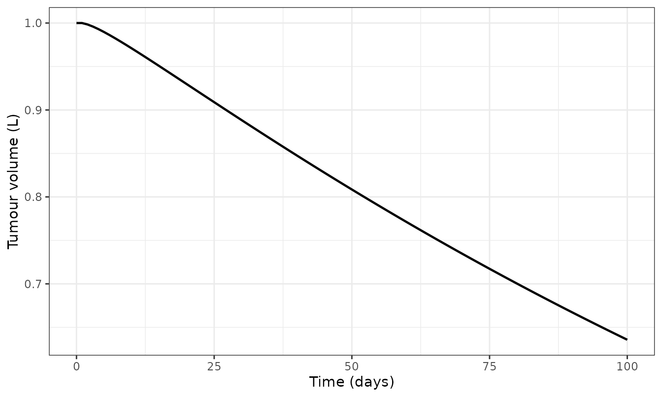
Replicates Figure 2 of Yates and Mistry (2023): time versus tumour volume for repeat dosing with the exponential model.
Repeat dosing against the Appendix S1 sum
Appendix S1 gives the exact effect integral after N
doses tau apart as a sum of logarithms of geometric
accumulation terms. Evaluated at the dosing times this must reproduce
the numerical solution exactly.
tau <- 7; N <- 8; D <- 2
s <- simulate_arm(mod_expo, D, seq(0, N * tau, by = 0.25), pars_fig2,
                  ii = tau, addl = N - 1)
a <- a_of(pars_fig2)
ii_seq <- seq_len(N)
acc <- (1 - exp(-a * ii_seq * tau)) / (1 - exp(-a * tau))
eff <- cumsum(log((1 + D * acc) / (1 + D * exp(-a * tau) * acc)))
tN <- ii_seq * tau
ana <- exp(pars_fig2[["lrbase"]]) *
  exp(exp(pars_fig2[["lp"]]) * tN - exp(pars_fig2[["lemax"]]) / a * eff)

repeat_check <- tibble(
  check = sprintf("Exponential, repeat dose (tau = %g, N = %d)", tau, N),
  max_rel_err = max(abs(s$tumor_vol[match(tN, s$time)] - ana) / ana)
)
repeat_check |> knitr::kable(digits = 16)| check | max_rel_err |
|---|---|
| Exponential, repeat dose (tau = 7, N = 8) | 3.592e-13 |
Replicates Figure 1 and Figure 3: dose-response versus PK half-life
Figures 1 and 3 sweep CL from 0.01 to 10 L/day
(i.e. sweep the PK half-life) at Vd = 1 and read tumour
volume off on day 14. Here Emax = 0.0025 < k, so the
drug can only slow growth and the response plateaus short of
shrinkage.
doses <- 10^seq(-2, 3, length.out = 40)
cl_grid <- c(0.01, 0.1, 1, 10)

dose_response <- expand_grid(cl = cl_grid, dose = doses,
                             regimen = c("Single dose", "Daily x 14")) |>
  rowwise() |>
  mutate(
    tumor_vol = {
      p <- replace(pars_fig1, "lcl", log(cl))
      s <- if (regimen == "Single dose") {
        simulate_arm(mod_expo, dose, c(0, 14), p)
      } else {
        simulate_arm(mod_expo, dose, c(0, 14), p, ii = 1, addl = 13)
      }
      s$tumor_vol[s$time == 14]
    }
  ) |>
  ungroup()

ggplot(dose_response, aes(dose, tumor_vol, colour = factor(cl))) +
  geom_line(linewidth = 0.8) +
  facet_wrap(~regimen) +
  scale_x_log10() +
  labs(x = "Dose", y = "Tumour volume at day 14 (L)",
       colour = "CL (L/day)") +
  theme_bw()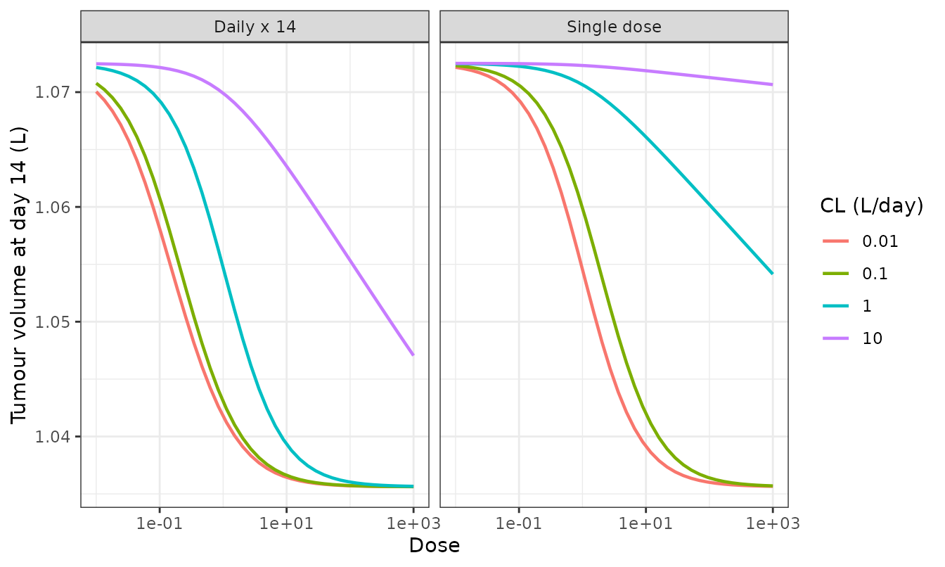
Replicates Figures 1 and 3 of Yates and Mistry (2023): dose-response after 14 days for single versus daily repeat dosing, as a function of PK half-life.
Two published conclusions are visible: the dose-response curve
left-shifts as PK half-life increases (smaller
CL), and repeat dosing left-shifts the curve further by
approximately the accumulation factor 1 - exp(-a*tau).
tau <- 1
tibble(cl = cl_grid) |>
  mutate(
    a = cl / 1,
    accumulation_factor = 1 / (1 - exp(-a * tau)),
    ed50_shift_predicted = accumulation_factor
  ) |>
  knitr::kable(digits = 4,
caption = "Predicted ED50 reduction on going from single to daily dosing (p. 1597).")| cl | a | accumulation_factor | ed50_shift_predicted |
|---|---|---|---|
| 0.01 | 0.01 | 100.5008 | 100.5008 |
| 0.10 | 0.10 | 10.5083 | 10.5083 |
| 1.00 | 1.00 | 1.5820 | 1.5820 |
| 10.00 | 10.00 | 1.0000 | 1.0000 |
Replicates Figure 4: q.d. versus b.d. dose fractionation
frac <- expand_grid(cl = cl_grid, daily_dose = doses) |>
  rowwise() |>
  mutate(
    qd = {
      p <- replace(pars_fig1, "lcl", log(cl))
      simulate_arm(mod_expo, daily_dose, c(0, 14), p, ii = 1, addl = 13) |>
        (\(s) s$tumor_vol[s$time == 14])()
    },
    bd = {
      p <- replace(pars_fig1, "lcl", log(cl))
      simulate_arm(mod_expo, daily_dose / 2, c(0, 14), p, ii = 0.5, addl = 27) |>
        (\(s) s$tumor_vol[s$time == 14])()
    }
  ) |>
  ungroup() |>
  pivot_longer(c(qd, bd), names_to = "schedule", values_to = "tumor_vol")

ggplot(frac, aes(daily_dose, tumor_vol, colour = schedule)) +
  geom_line(linewidth = 0.8) +
  facet_wrap(~paste0("CL = ", cl)) +
  scale_x_log10() +
  labs(x = "Total daily dose", y = "Tumour volume at day 14 (L)",
       colour = "Schedule") +
  theme_bw()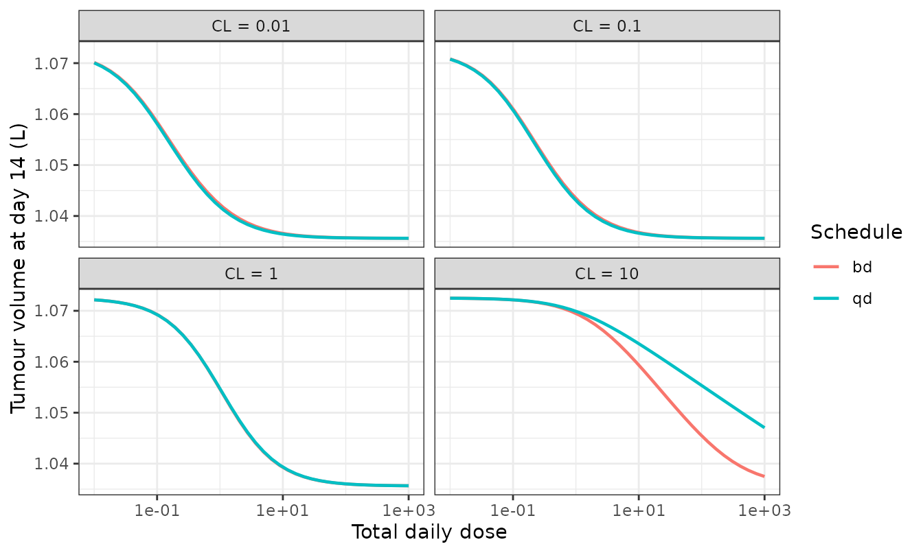
Replicates Figure 4 of Yates and Mistry (2023): q.d. versus b.d. dosing at matched total daily dose.
The paper’s algebra concludes b.d. is always at least as effective as q.d. at matched total daily dose, but that the gain is marginal, especially for long-half-life drugs. That proof is about the long-time asymptotic effect per dose, in which the accumulation factor has reached steady state (p. 1597). Test the paper’s claim on its own terms first: b.d. wins iff
(AFqd - AFbd) / AFbd^2 < D / (Vd * EC50), with
AFqd = 1/(1 - exp(-a*tau)) and
AFbd = 1/(1 - exp(-a*tau/2)).
asymptotic_effect <- function(p, D, tau, n_doses) {
  a <- a_of(p); vd <- exp(p[["lvc"]]); ec50 <- exp(p[["lec50"]])
  em <- exp(p[["lemax"]])
  af_qd <- 1 / (1 - exp(-a * tau))
  af_bd <- 1 / (1 - exp(-a * tau / 2))
  tibble(
    `CL (L/day)` = exp(p[["lcl"]]),
    Dose = D,
    Eqd = (ec50 / (ec50 + D / vd * af_qd))^(em * n_doses / a),
    Ebd = (ec50 / (ec50 + D / (2 * vd) * af_bd))^(em * 2 * n_doses / a),
    `(AFqd - AFbd)/AFbd^2` = (af_qd - af_bd) / af_bd^2,
    `D/(Vd*EC50)` = D / (vd * ec50)
  )
}

asym <- expand_grid(cl = cl_grid, dose = doses) |>
  rowwise() |>
  reframe(asymptotic_effect(replace(pars_fig1, "lcl", log(cl)),
                            dose, tau = 1, n_doses = 14))

## The paper's inequality, and its consequence, must hold at every point.
stopifnot(all(asym$`(AFqd - AFbd)/AFbd^2` < asym$`D/(Vd*EC50)`))
stopifnot(all(asym$Ebd < asym$Eqd))

asym |>
  group_by(`CL (L/day)`) |>
  summarise(`max b.d. advantage in effect per dose (%)` =
              100 * max((Eqd - Ebd) / Eqd), .groups = "drop") |>
knitr::kable(digits = 4)| CL (L/day) | max b.d. advantage in effect per dose (%) |
|---|---|
| 0.01 | 100.0000 |
| 0.10 | 96.0194 |
| 1.00 | 21.5354 |
| 10.00 | 1.9196 |
The asymptotic claim holds exactly, everywhere. Now the finite-time ODE, which is what the figure above shows: 14 days of dosing started from a drug-free state, so the accumulation factor has not reached steady state for the slowly-cleared arms.
frac_wide <- frac |>
  pivot_wider(names_from = schedule, values_from = tumor_vol) |>
  mutate(pct_gain = 100 * (qd - bd) / qd)

frac_summary <- frac_wide |>
  group_by(cl) |>
  summarise(`max b.d. advantage (%)` = max(pct_gain),
            `worst q.d. advantage (%)` = max(-pct_gain),
            .groups = "drop") |>
  rename("CL (L/day)" = cl)

## Fast clearance reaches the asymptotic regime within 14 days and shows a
## clear b.d. advantage; slow clearance has not accumulated to steady state,
## and there the two schedules are numerically indistinguishable.
stopifnot(frac_summary$`max b.d. advantage (%)`[frac_summary$`CL (L/day)` == 10] > 1)
stopifnot(all(frac_summary$`worst q.d. advantage (%)`[frac_summary$`CL (L/day)` < 10] < 0.05))

knitr::kable(frac_summary, digits = 5)| CL (L/day) | max b.d. advantage (%) | worst q.d. advantage (%) |
|---|---|---|
| 0.01 | -0.00017 | 0.04672 |
| 0.10 | -0.00017 | 0.04205 |
| 1.00 | 0.01255 | 0.00293 |
| 10.00 | 1.02723 | -0.00001 |
The b.d. advantage is largest for the fastest-cleared drug
(CL = 10, ~1%) and vanishes for the slowest
(CL = 0.01), exactly as the paper argues. Over this finite
14-day window the slow-clearance arms in fact favour q.d. by under 0.05%
– a transient effect of the first dose being twice as large under q.d.,
not a contradiction of the paper’s steady-state result. See Errata.
Nadir time and nadir depth
For a single dose with Emax > k the paper gives the
nadir time t = -(1/a) * ln(k*EC50*Vd / (D*(Emax - k))),
real only when D > EC50*Vd / (Emax/k - 1), and a closed
form for Vnadir/V0.
p <- pars_fig2
a <- a_of(p)
k <- exp(p[["lp"]]); Em <- exp(p[["lemax"]])
ec50 <- exp(p[["lec50"]]); vd <- exp(p[["lvc"]])
d_min <- ec50 * vd / (Em / k - 1)

nadir <- lapply(c(2, 10), function(D) {
  t_ana <- -1 / a * log(k * ec50 * vd / (D * (Em - k)))
  s <- simulate_arm(mod_expo, D, seq(0, 400, by = 0.05), p)
  A <- D / (ec50 * vd)
  v_ana <- ((Em / k - 1)^k * (Em / (Em - k))^Em *
              (A^(k / Em) / (1 + A))^Em)^(1 / a)
  tibble(Dose = D,
         `t nadir (analytic, day)` = t_ana,
         `t nadir (numeric, day)` = s$time[which.min(s$tumor_vol)],
         `Vnadir/V0 (analytic)` = v_ana,
         `Vnadir/V0 (numeric)` = min(s$tumor_vol) / exp(p[["lrbase"]]))
}) |> bind_rows()

stopifnot(all(abs(nadir$`Vnadir/V0 (analytic)` - nadir$`Vnadir/V0 (numeric)`) /
                nadir$`Vnadir/V0 (analytic)` < 1e-6))
stopifnot(all(nadir$Dose > d_min))

knitr::kable(nadir, digits = 6,
caption = sprintf("Nadir exists only for D > %.4f.", d_min))| Dose | t nadir (analytic, day) | t nadir (numeric, day) | Vnadir/V0 (analytic) | Vnadir/V0 (numeric) |
|---|---|---|---|---|
| 2 | 69.31472 | 69.30 | 0.942809 | 0.942809 |
| 10 | 230.25851 | 230.25 | 0.574960 | 0.574960 |
The nadir time is logarithmic in dose, as the paper states.
PKNCA check on the pharmacokinetic layer
The paper’s “AUC-driven” result (p. 1596) follows from the Taylor
expansion
(Emax/a)*ln(1 + D/(Vd*EC50)) ~ (Emax/a)*(D/CL) = (Emax/a)*AUC,
which relies on AUC = D / CL for the one-compartment bolus.
Confirm that identity with PKNCA.
pk_doses <- c(1, 5, 25)

conc <- lapply(pk_doses, function(D) {
  simulate_arm(mod_expo, D, seq(0, 2000, by = 1), pars_fig2) |>
    mutate(id = 1L, treatment = paste0("D = ", D))
}) |>
  bind_rows() |>
  filter(!is.na(Cc))

dose_df <- tibble(id = 1L,
                  treatment = paste0("D = ", pk_doses),
                  time = 0,
                  amt = pk_doses)

conc_obj <- PKNCA::PKNCAconc(conc, Cc ~ time | treatment + id,
                             concu = "dose unit/L", timeu = "day")
dose_obj <- PKNCA::PKNCAdose(dose_df, amt ~ time | treatment + id,
                             doseu = "dose unit")

res <- suppressWarnings(PKNCA::pk.nca(PKNCA::PKNCAdata(
  conc_obj, dose_obj,
  intervals = data.frame(start = 0, end = Inf,
                         aucinf.obs = TRUE, cmax = TRUE, half.life = TRUE)
)))

nca <- as.data.frame(res) |>
  filter(start == 0, end == Inf) |>
  select(treatment, PPTESTCD, PPORRES) |>
  pivot_wider(names_from = PPTESTCD, values_from = PPORRES) |>
  left_join(dose_df |> select(treatment, amt), by = "treatment") |>
  mutate(auc_pred = amt / 0.01,
         cmax_pred = amt / 1,
         thalf_pred = log(2) / 0.01)

nca |>
  select(Regimen = treatment,
         `AUC0-inf (simulated)` = aucinf.obs,
         `AUC0-inf (D/CL)` = auc_pred,
         `Cmax (simulated)` = cmax,
         `Cmax (D/Vd)` = cmax_pred,
         `t1/2 (simulated)` = half.life,
         `t1/2 (ln2/a)` = thalf_pred) |>
knitr::kable(digits = 4)| Regimen | AUC0-inf (simulated) | AUC0-inf (D/CL) | Cmax (simulated) | Cmax (D/Vd) | t1/2 (simulated) | t1/2 (ln2/a) |
|---|---|---|---|---|---|---|
| D = 1 | 100 | 100 | 1 | 1 | 69.3147 | 69.3147 |
| D = 25 | 2500 | 2500 | 25 | 25 | 69.3147 | 69.3147 |
| D = 5 | 500 | 500 | 5 | 5 | 69.3147 | 69.3147 |
Case study 2: Mayneord linear radial growth
Appendix S1 gives
V(T) = (k/3*T + V0^(1/3) - Emax/(3a) * ln((EC50 + D/Vd)/(EC50 + (D/Vd)*exp(-a*T))))^3.
pars_fig5 <- c(lcl = log(0.01), lvc = log(1), lrbase = log(1),
               lp = log(0.005), lemax = log(0.01), lec50 = log(1))

mayn_check <- lapply(c(0.5, 2, 20), function(D) {
  s <- simulate_arm(mod_mayn, D, tt, pars_fig5)
  a <- a_of(pars_fig5)
  ana <- (exp(pars_fig5[["lp"]]) / 3 * s$time + exp(pars_fig5[["lrbase"]])^(1 / 3) -
            exp(pars_fig5[["lemax"]]) / (3 * a) *
            log((1 + D) / (1 + D * exp(-a * s$time))))^3
  tibble(check = sprintf("Mayneord, single dose D = %g", D),
         max_rel_err = max(abs(s$tumor_vol - ana) / ana))
}) |> bind_rows()

## Repeat dosing.
tau <- 7; N <- 8; D <- 2
s <- simulate_arm(mod_mayn, D, seq(0, N * tau, by = 0.25), pars_fig5,
                  ii = tau, addl = N - 1)
a <- a_of(pars_fig5)
ii_seq <- seq_len(N)
acc <- (1 - exp(-a * ii_seq * tau)) / (1 - exp(-a * tau))
eff <- cumsum(log((1 + D * acc) / (1 + D * exp(-a * tau) * acc)))
tN <- ii_seq * tau
ana <- (exp(pars_fig5[["lp"]]) / 3 * tN + 1 -
          exp(pars_fig5[["lemax"]]) / (3 * a) * eff)^3

mayn_check <- bind_rows(
  mayn_check,
  tibble(check = sprintf("Mayneord, repeat dose (tau = %g, N = %d)", tau, N),
         max_rel_err = max(abs(s$tumor_vol[match(tN, s$time)] - ana) / ana))
)

mayn_check |> knitr::kable(digits = 16)| check | max_rel_err |
|---|---|
| Mayneord, single dose D = 0.5 | 7.70e-15 |
| Mayneord, single dose D = 2 | 3.50e-14 |
| Mayneord, single dose D = 20 | 1.00e-14 |
| Mayneord, repeat dose (tau = 7, N = 8) | 1.12e-13 |
fig5 <- lapply(cl_grid, function(cl) {
  simulate_arm(mod_mayn, 1, seq(0, 100, by = 0.5),
               replace(pars_fig5, "lcl", log(cl)), ii = 1, addl = 99) |>
    mutate(cl = cl)
}) |> bind_rows()

ggplot(fig5, aes(time, tumor_vol, colour = factor(cl))) +
  geom_line(linewidth = 0.8) +
  labs(x = "Time (days)", y = "Tumour volume (L)", colour = "CL (L/day)") +
  theme_bw()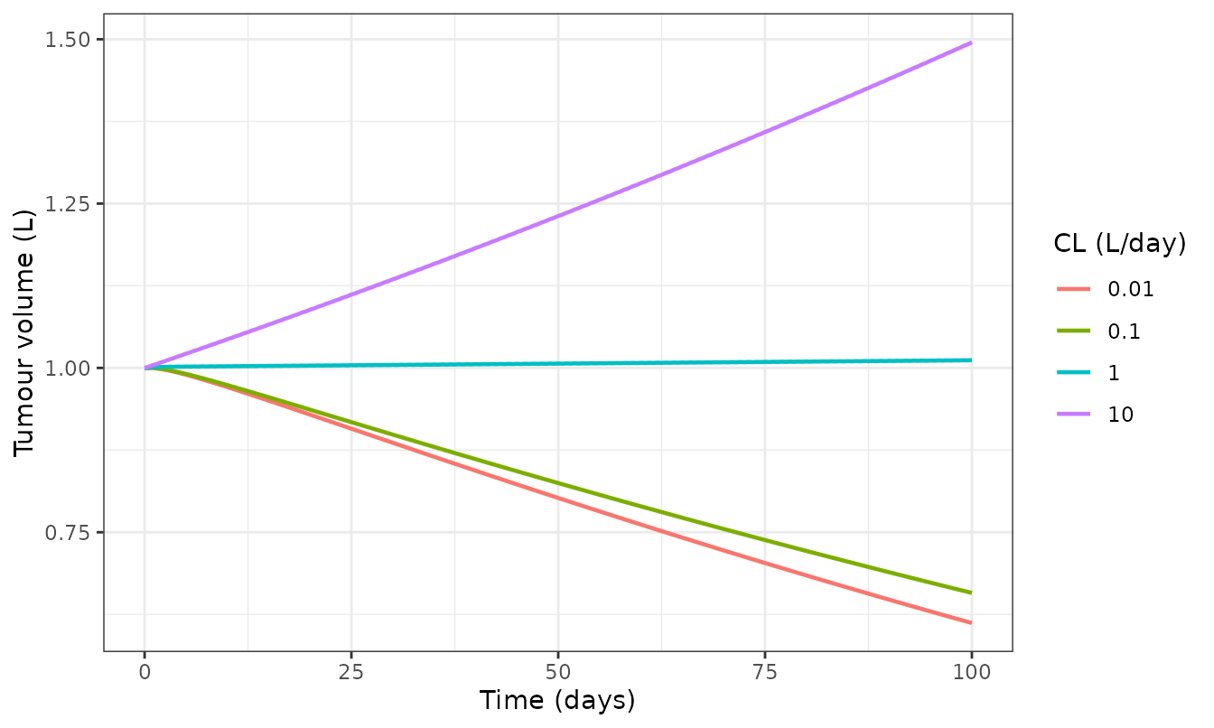
Replicates Figure 5 of Yates and Mistry (2023): time versus volume for repeat dosing with the Mayneord model.
The paper notes that at large time the Mayneord drug effect tends to
Emax/(3a) * ln(1 + D/(Vd*EC50)), giving a
log-linear rather than sigmoidal dose-response. Figure
6 compares single and repeat dosing.
pars_fig6 <- replace(pars_fig5, "lemax", log(0.0025))

fig6 <- expand_grid(cl = cl_grid, dose = doses,
                    regimen = c("Single dose", "Daily x 14")) |>
  rowwise() |>
  mutate(tumor_vol = {
    p <- replace(pars_fig6, "lcl", log(cl))
    s <- if (regimen == "Single dose") {
      simulate_arm(mod_mayn, dose, c(0, 14), p)
    } else {
      simulate_arm(mod_mayn, dose, c(0, 14), p, ii = 1, addl = 13)
    }
    s$tumor_vol[s$time == 14]
  }) |>
  ungroup()

ggplot(fig6, aes(dose, tumor_vol, colour = factor(cl))) +
  geom_line(linewidth = 0.8) +
  facet_wrap(~regimen) +
  scale_x_log10() +
  labs(x = "Dose", y = "Tumour volume at day 14 (L)", colour = "CL (L/day)") +
  theme_bw()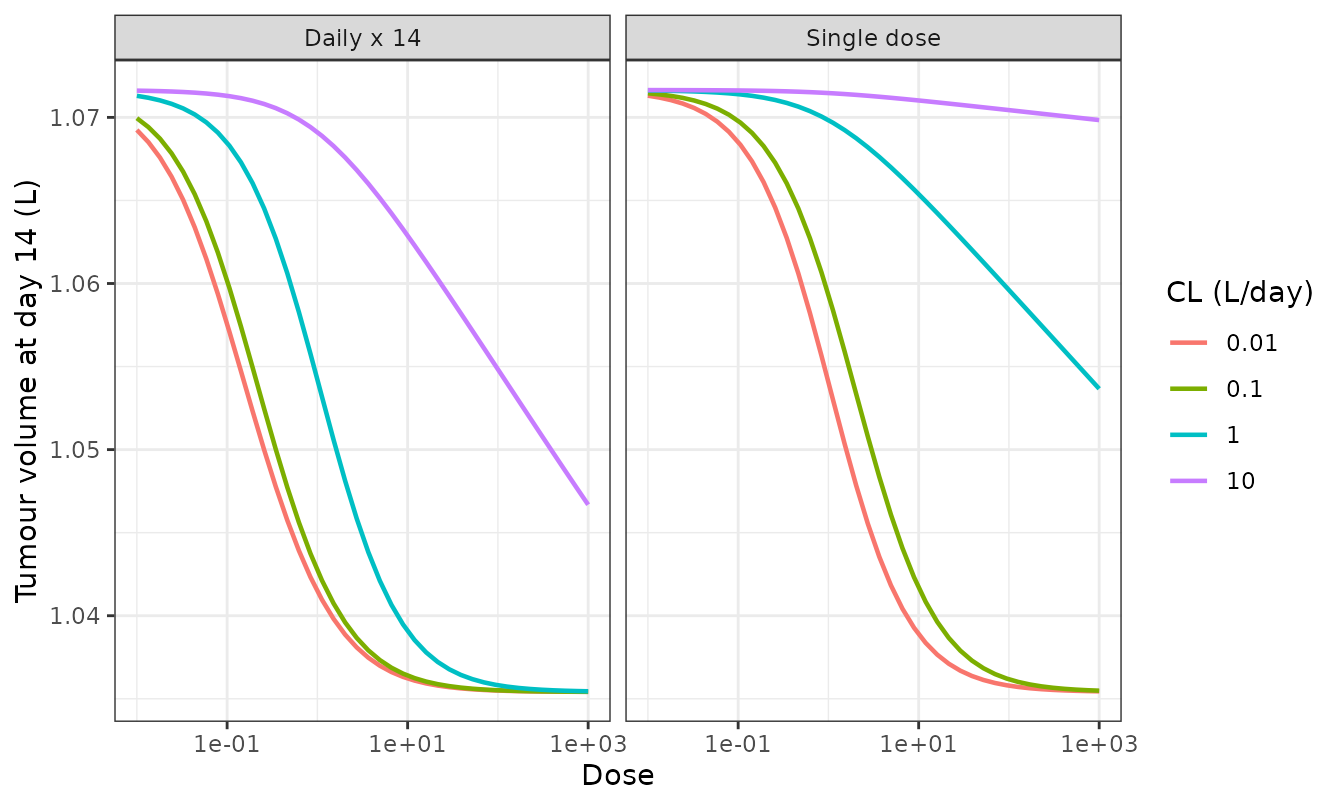
Replicates Figure 6 of Yates and Mistry (2023): single versus repeat dose for the Mayneord model.
Case study 3: von Bertalanffy
The untreated model has the closed form
V(t) = (k/kd + (V0^(1/3) - k/kd) * exp(-kd*t/3))^3,
plateauing at (k/kd)^3.
pars_fig7 <- c(lcl = log(0.01), lvc = log(1), lrbase = log(1),
               lp = log(0.005), lkdeath = log(0.004),
               lemax = log(0.01), lec50 = log(1))

kk <- exp(pars_fig7[["lp"]]) / exp(pars_fig7[["lkdeath"]])
s0 <- simulate_arm(mod_bert, 0, tt, pars_fig7)
ana0 <- (kk + (1 - kk) * exp(-exp(pars_fig7[["lkdeath"]]) / 3 * s0$time))^3

bert_check <- tibble(
  check = "Bertalanffy, no drug",
  max_rel_err = max(abs(s0$tumor_vol - ana0) / ana0)
)

## Long-run plateau.
s_long <- simulate_arm(mod_bert, 0, seq(0, 20000, by = 50), pars_fig7)
plateau_rel_err <- abs(tail(s_long$tumor_vol, 1) - kk^3) / kk^3
stopifnot(plateau_rel_err < 1e-6)
The treated model’s Appendix S1 solution is an infinite series that
converges only for D / (EC50 * Vd) < 1; the ODE encoded
in the model file carries no such restriction, so the series is used
only as a validation target within its domain.
a <- a_of(pars_fig7)
r <- exp(pars_fig7[["lkdeath"]]) / (3 * a)
nn <- 0:400

bert_check <- bind_rows(bert_check, lapply(c(0.25, 0.5, 0.9), function(D) {
  s <- simulate_arm(mod_bert, D, tt, pars_fig7)
  A <- D / (exp(pars_fig7[["lec50"]]) * exp(pars_fig7[["lvc"]]))
  ser <- vapply(s$time, function(ti) {
    sum((-1)^nn / (nn - r + 1) * A^(nn + 1) *
          (1 - exp(-a * (nn - r + 1) * ti)))
  }, numeric(1))
  ana <- (kk + (1 - kk - exp(pars_fig7[["lemax"]]) / (3 * a) * ser) *
            exp(-exp(pars_fig7[["lkdeath"]]) / 3 * s$time))^3
  tibble(check = sprintf("Bertalanffy + drug, D = %g (D/(EC50*Vd) = %.2f)", D, A),
         max_rel_err = max(abs(s$tumor_vol - ana) / ana))
}) |> bind_rows())

bert_check |> knitr::kable(digits = 16)| check | max_rel_err |
|---|---|
| Bertalanffy, no drug | 3.610e-14 |
| Bertalanffy + drug, D = 0.25 (D/(EC50*Vd) = 0.25) | 1.566e-13 |
| Bertalanffy + drug, D = 0.5 (D/(EC50*Vd) = 0.50) | 2.186e-13 |
| Bertalanffy + drug, D = 0.9 (D/(EC50*Vd) = 0.90) | 2.439e-13 |
fig7 <- lapply(c(0, 0.25, 0.5, 0.9), function(D) {
  simulate_arm(mod_bert, D, seq(0, 600, by = 2), pars_fig7) |>
    mutate(dose = paste0("D = ", D))
}) |> bind_rows()

ggplot(fig7, aes(time, tumor_vol, colour = dose)) +
  geom_line(linewidth = 0.8) +
  labs(x = "Time (days)", y = "Tumour volume (L)", colour = NULL) +
  theme_bw()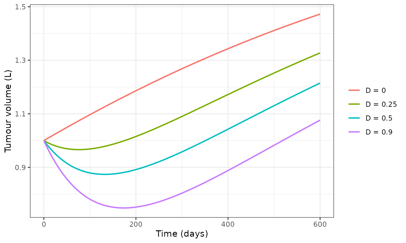
Replicates Figure 7 of Yates and Mistry (2023): time-dependent response of the Bertalanffy model after a single dose.
Overall known-answer summary
Every numerically integrated model reproduces the paper’s own closed-form solution to solver tolerance.
all_checks <- bind_rows(expo_check, hill_check, repeat_check,
                        mayn_check, bert_check)

stopifnot(all(all_checks$max_rel_err < 1e-8))

all_checks |>
  rename("Known-answer check" = check,
         "Max relative error" = max_rel_err) |>
knitr::kable(digits = 16)| Known-answer check | Max relative error |
|---|---|
| Exponential, single dose D = 0.5 | 3.440e-14 |
| Exponential, single dose D = 2 | 5.220e-14 |
| Exponential, single dose D = 20 | 8.260e-14 |
| Exponential, Hill n = 2 | 1.689e-13 |
| Exponential, Hill n = 3 | 4.283e-13 |
| Exponential, repeat dose (tau = 7, N = 8) | 3.592e-13 |
| Mayneord, single dose D = 0.5 | 7.700e-15 |
| Mayneord, single dose D = 2 | 3.500e-14 |
| Mayneord, single dose D = 20 | 1.000e-14 |
| Mayneord, repeat dose (tau = 7, N = 8) | 1.120e-13 |
| Bertalanffy, no drug | 3.610e-14 |
| Bertalanffy + drug, D = 0.25 (D/(EC50*Vd) = 0.25) | 1.566e-13 |
| Bertalanffy + drug, D = 0.5 (D/(EC50*Vd) = 0.50) | 2.186e-13 |
| Bertalanffy + drug, D = 0.9 (D/(EC50*Vd) = 0.90) | 2.439e-13 |
Assumptions and deviations
-
No data were fitted. Yates and Mistry (2023) is a
theoretical / tutorial paper. Every parameter is an illustrative
constant taken verbatim from the figure captions and is encoded with
fixed(). The models therefore carry no inter-individual variability and no residual-error model; none is reported anywhere in the source, and inventing one would be fabrication. Consequentlypopulation$n_subjectsandpopulation$n_studiesare 0 andpopulation$speciesis recorded as not applicable. -
PK encoded as an ODE, not as the printed analytic
expression. The paper writes
C(t) = (D/Vd)*exp(-a*t). The model files integrate the equivalent one-compartment ODEd/dt(central) = -kel*centralwithCc = central/vcandkel = cl/vc. This is mathematically identical for a bolus dose and makes the paper’s repeat-dose and accumulation results follow directly from ordinaryii/addldosing records. The known-answer checks above confirm the equivalence to ~1e-13 relative error. -
Default parameter sets. Each model file defaults to
the parameter set of its own time-course figure (Figure 2 for
exponential, Figure 5 for Mayneord, Figure 7 for Bertalanffy). The
dose-response figures (1, 3, 4, 6) use
Emax = 0.0025instead of0.01; this vignette overrideslemaxexplicitly where those figures are reproduced. -
Hill coefficient defaults to 1. Every published
figure uses the plain Emax form. The paper presents the
Hill-
nform as a generalisation of the same case study rather than as a separate model, so it is encoded as afixed(log(1))parameter inYates_2023_tgi_exponentialthat the user can change, rather than as a fourth model file. -
Units. The paper works in “units of days and
litres” and never names a drug or a mass unit. Dose therefore carries an
arbitrary mass unit and concentration is that unit per litre.
Emaxis a rate:1/dayin the exponential model, butL^(1/3)/dayin the Mayneord and Bertalanffy models, where it acts on the tumour radius (the paper notes[Emax] = L.T^-1and[Emax/a] = L, p. 1598). -
Bertalanffy series solution has a restricted
domain. The published closed-form solution converges only for
D/(EC50*Vd) < 1(p. 1599). This is a limitation of the derivation, not of the model; the ODE integrates fine at any dose, so the series is used here only as a validation target inside its domain of validity. - No repeat-dose expression is published for the Bertalanffy model. The paper states such expressions “will be significantly more complex” and does not derive them, so no repeat-dose known-answer check is possible for that case study. The ODE itself supports repeat dosing normally.
Errata
-
The main text’s ED50 expression is inconsistent with
Appendix S1 and with the paper’s own Equation (4). On p. 1595
the main text states that the ED50 “in this case is
(EC50 V)^(a/Emax)”. Raising a concentration-times-volume quantity to a dimensionless power is not dimensionally coherent, and Appendix S1 instead states that “the ED50 in this case isKV”, i.e.EC50 * Vd(the supplement writesKforEC50throughout that passage). Working directly from the long-time solution (Eq. 4), the effect factor isE(D) = (EC50/(EC50 + D/Vd))^(Emax/a), so:-
D = EC50*Vdis the dose at which the sigmoid’s argument is halved, which matches the Appendix statement and is the curve’s location parameter inD/(Vd*EC50)space; whereas - the dose giving exactly half the maximal effect is
D = Vd*EC50*(2^(a/Emax) - 1).
a/Emax = 1. All three published readings agree numerically for the Figure 2 parameter set purely becauseEC50 = Vd = 1anda/Emax = 1there, which is why the discrepancy is easy to miss. -
ed50_compare <- function(p) {
  a <- a_of(p); ec50 <- exp(p[["lec50"]]); vd <- exp(p[["lvc"]])
  Ef <- function(D) (ec50 / (ec50 + D / vd))^(exp(p[["lemax"]]) / a)
  tibble(
    `a/Emax` = a / exp(p[["lemax"]]),
    `Appendix S1: EC50*Vd` = ec50 * vd,
    `E at that dose` = Ef(ec50 * vd),
    `Exact half-effect dose` = vd * ec50 * (2^(a / exp(p[["lemax"]])) - 1),
    `E at that dose ` = Ef(vd * ec50 * (2^(a / exp(p[["lemax"]])) - 1)),
    `Main text: (EC50*Vd)^(a/Emax)` = (ec50 * vd)^(a / exp(p[["lemax"]])),
    `E at that dose  ` = Ef((ec50 * vd)^(a / exp(p[["lemax"]])))
  )
}

bind_rows(
  ed50_compare(pars_fig2) |> mutate(`Parameter set` = "Figure 2 (Emax = 0.01)"),
  ed50_compare(pars_fig1) |> mutate(`Parameter set` = "Figure 1 (Emax = 0.0025)")
) |>
  relocate(`Parameter set`) |>
knitr::kable(digits = 4)| Parameter set | a/Emax | Appendix S1: EC50*Vd | E at that dose | Exact half-effect dose | E at that dose | Main text: (EC50*Vd)^(a/Emax) | E at that dose |
|---|---|---|---|---|---|---|---|
| Figure 2 (Emax = 0.01) | 1 | 1 | 0.5000 | 1 | 0.5 | 1 | 0.5000 |
| Figure 1 (Emax = 0.0025) | 4 | 1 | 0.8409 | 15 | 0.5 | 1 | 0.8409 |
Only the “exact half-effect dose” column returns E = 0.5
in both parameter sets. This affects a narrative aside only; no model
equation or parameter value depends on it.
The dose-fractionation proof is asymptotic, and the b.d. advantage does not survive a finite dosing window for long-half-life drugs. On p. 1597 the paper concludes that b.d. dosing is more effective than q.d. at matched total daily dose and that this is “always true”. That proof compares the long-time effect-per-dose expressions, in which the accumulation factor has reached steady state. The
fractionation-asymptoticchunk above confirms the inequality holds exactly at every point tested. However, the 14-day ODE simulation that Figure 4 depicts starts from a drug-free state, so the slowly-cleared arms (CL= 0.01-1 L/day, half-lives of 17-69 days) have not accumulated to steady state by day 14. In that transient the two schedules are numerically indistinguishable, and q.d. is marginally better – by less than 0.05% – because its first dose is twice as large. This is not an error in the paper’s algebra; it is a reminder that the asymptotic result needs several half-lives of dosing before it applies, which reinforces the paper’s own point about the time of endpoint assessment mattering.The dose-fractionation section mixes hours and days. The accumulation factors on p. 1597 are written
AFq.d. = 1/(1 - e^(-24a))andAFb.d. = 1/(1 - e^(-12a)), i.e. withtauin hours, while every figure caption states the parameters are “units of days and liters” anda = CL/Vdis therefore in 1/day. Taken literally the printed expressions describe a 24-day and 12-day interval. The vignette usestau= 1 day and 0.5 day, which is the intended q.d. / b.d. comparison; the algebraic conclusion is unaffected because the inequality holds for anyaandtau.Figure captions 2-7 print “
V0, xxx” in the abbreviation list, an unresolved placeholder from typesetting. Figure 1’s caption gives the intended expansion, “V0, initial tumor volume”.No erratum or corrigendum was found for this article on the journal landing page or in PubMed at the time of extraction.
Reference
Yates JWT, Mistry HB. Skipping a pillar does not make for strong foundations: Pharmacokinetic-pharmacodynamic reasoning behind the shape of dose-response relationships in oncology. CPT Pharmacometrics Syst Pharmacol. 2023;12:1591-1601. doi:10.1002/psp4.13020