Interleukin-6 driven CYP modulation after talquetamab (Willemin 2024)
Source:vignettes/articles/Willemin_2024_interleukin6_cyp_talquetamab.Rmd
Willemin_2024_interleukin6_cyp_talquetamab.RmdModel and source
- Citation: Willemin ME, Gong J, Hilder BW, Masterson T, Tolbert J, Renaud T, Heuck C, Kane C, De Zwart L, Girgis S, Ma X, Ouellet D. Evaluation of Drug-Drug Interaction Potential of Talquetamab, a T-Cell-Redirecting GPRC5D x CD3 Bispecific Antibody, as a Result of Cytokine Release Syndrome in Patients with Relapsed/Refractory Multiple Myeloma in MonumenTAL-1, Using a Physiologically Based Pharmacokinetic Model. Target Oncol. 2024;19(6):965-979. doi:10.1007/s11523-024-01093-6. IL-6 disposition recovered from the simulated profiles of Figs 1 and 2; hepatic CYP turnover rate constants recovered from the activity time courses of Figs 3 and 4 and gated against Table 3. The IL-6 model itself is stated by this paper to be the previously published one of Willemin ME et al. CPT Pharmacometrics Syst Pharmacol. 2024;13(7):1117-1129 (doi:10.1002/psp4.13144), from which the interaction potencies (Indmax, IndC50) are carried; those in turn are attributed to Dickmann LJ et al. Drug Metab Dispos. 2011;39:1415-1422 and Jiang X et al. AAPS J. 2016;18:767-776, and the turnover equation form to Machavaram KK et al. Clin Pharmacol Ther. 2013;94:260-268.
- Article: https://doi.org/10.1007/s11523-024-01093-6 (PMC11557650)
Willemin 2024 is a Janssen Research & Development analysis submitted to the FDA and the EMA in support of the talquetamab filing. Talquetamab is a GPRC5D x CD3 bispecific antibody; in the MonumenTAL-1 study most patients treated at either recommended phase 2 dose (RP2D) experienced cytokine release syndrome (CRS), which transiently elevates interleukin-6 (IL-6). Because IL-6 suppresses several cytochrome P450 enzymes, the analysis asks how much that transient elevation can perturb the exposure of concomitant CYP substrates, and for how long.
Talquetamab is never modelled. IL-6 is an endogenous protein, so its appearance in the body was represented by intravenous infusions whose schedule the authors “adjusted to recover the observed IL-6 kinetics profile for each of the scenarios”. What is extracted here is therefore an IL-6 exposure driver coupled to five hepatic CYP turnover pools – the reusable, mechanistically specified part of the paper – and not a talquetamab PK model.
Four published scenarios are reproduced, two per dosing schedule:
| Scenario | Schedule | IL-6 profile | IL-6 | Cycle 1 begins |
|---|---|---|---|---|
qw_median |
0.4 mg/kg QW | median across patients | 18.4 pg/mL | 96 h |
qw_max |
0.4 mg/kg QW | patient with the highest | 213 pg/mL | 96 h |
q2w_median |
0.8 mg/kg Q2W | median across patients | 7.07 pg/mL | 168 h |
q2w_max |
0.8 mg/kg Q2W | patient with the highest | 3503 pg/mL | 168 h |
Time zero throughout is the first step-up dose, which is the time origin of Figs 1–4. Table 3 instead quotes its timings relative to the start of cycle 1 (the first full treatment dose), which the Methods place 96 h after the first step-up dose on the QW schedule and 168 h after it on the Q2W schedule. Every comparison against Table 3 below converts explicitly between the two.
Population
pop <- rxode2::rxode2(readModelDb("Willemin_2024_interleukin6_cyp_talquetamab"))$meta$population
#> ℹ parameter labels from comments will be replaced by 'label()'
tibble::tibble(Field = names(pop), Value = vapply(pop, as.character, character(1))) |>
knitr::kable()| Field | Value |
|---|---|
| species | human |
| n_subjects | 195 |
| n_studies | 1 |
| age_range | 20-50 years (Simcyp healthy-volunteer simulation population) |
| sex_female_pct | 50 |
| disease_state | relapsed/refractory multiple myeloma with cytokine release syndrome (source of the observed IL-6 data); the simulations themselves were run in a healthy-volunteer population |
| dose_range | talquetamab 0.01 and 0.06 mg/kg step-up doses then 0.4 mg/kg subcutaneous weekly; or 0.01, 0.06 and 0.3 mg/kg step-up doses then 0.8 mg/kg subcutaneous every other week (the IL-6 source regimens). IL-6 itself is dosed as a series of zero-order IV infusions. |
| regions | MonumenTAL-1 was a multinational phase I/II study (NCT03399799 / NCT04634552) |
| notes | Observed IL-6 concentration-time data come from 100 patients in the 0.4 mg/kg weekly cohort and 95 patients in the 0.8 mg/kg every-other-week cohort who experienced cytokine release syndrome and who either received no tocilizumab in cycle 1 or whose IL-6 Cmax occurred before tocilizumab was given. Two IL-6 scenarios are modelled per dosing schedule: scenario 1 is the median IL-6 profile (Cmax 18.4 pg/mL weekly, 7.07 pg/mL every other week) and scenario 2 is the single patient with the highest observed IL-6 Cmax (213 and 3503 pg/mL respectively). Prospective simulations used five trials of 100 subjects aged 20-50 years, 50 percent female. Cycle 1 (the first full treatment dose) begins 96 h after the first step-up dose on the weekly schedule and 168 h after it on the every-other-week schedule; those are the time origins for the Table 3 enzyme-activity timings. |
Source trace
Every ini() value, with where it comes from. This paper
is unusual in reporting no parameter table at all –
Tables 1–3 are simulation outputs (exposure ratios and
enzyme-activity extrema), and the IL-6 model is cited rather than
restated. The provenance below is therefore explicit about which values
are recovered from this paper’s own figures, and which are carried from
the IL-6 model this paper says it uses.
| Quantity | ini() name | Source |
|---|---|---|
| IL-6 clearance | lcl | Recovered from the simulated IL-6 profiles of Figs 1-2 (kel = 0.0411 /h), scaled by vc |
| IL-6 central volume | lvc | Vss 0.43 L/kg of the cited IL-6 model, divided by the Vss/Vc = 1.540 recovered from Figs 1-2 |
| IL-6 intercompartmental CL | lq | Recovered from Figs 1-2 (k12 = 0.0236 /h), scaled by vc |
| IL-6 peripheral volume | lvp | Vss 0.43 L/kg minus vc; gives k21 = 0.0437 /h |
| CYP1A2 Indmax - 1 / IndC50 | emax_1a2, ec50_1a2 | Carried from the IL-6 model this paper states it uses (Sect. 2.2); confirmed against this paper’s own Fig 3a plateau |
| CYP2C9 Indmax - 1 / IndC50 | emax_2c9, ec50_2c9 | As above |
| CYP2C19 Indmax - 1 / IndC50 | emax_2c19, ec50_2c19 | As above |
| CYP3A4 Indmax - 1 / IndC50 | emax_3a4, ec50_3a4 | As above |
| CYP3A5 Indmax - 1 / IndC50 | emax_3a5, ec50_3a5 | As above; the source model sets CYP3A5 equal to CYP3A4 |
| CYP1A2 turnover | kdeg_1a2 | Recovered from the CYP1A2 activity time courses of Figs 3a, 3b and 4a |
| CYP2C9 turnover | kdeg_2c9 | Recovered from the CYP2C9 activity time courses of Figs 3a, 3b and 4a |
| CYP2C19 turnover | kdeg_2c19 | Recovered from the CYP2C19 activity time courses of Figs 3a, 3b and 4a |
| CYP3A4 turnover | kdeg_3a4 | Recovered from the CYP3A4/CYP3A5 activity time courses of Figs 3a, 3b and 4a |
| CYP3A5 turnover | kdeg_3a5 | Recovered together with CYP3A4 |
| IIV on IL-6 CL and V | etalcl, etalvc | CV 50% carried from the cited IL-6 model; magnitude corroborated by the 90% CI band of this paper’s Fig 1a |
| Residual error | propSd | Not reported (simulation-only analysis); fixed at zero |
| IL-6 infusion schedules | (vignette) | Recovered from Figs 1-2, with peaks anchored to the Cmax values stated in the Table 1 footnotes |
The IL-6 driver
The paper never publishes the IL-6 infusion schedules it used. Each schedule was therefore recovered here from the paper’s own simulated IL-6 curve for that scenario: the infusion start and stop times were read from the slope changes of Figs 1–2, the rates were solved for by (non-negative) least squares against the digitized curve, and one disposition was fitted jointly across all four scenarios so that no scenario gets a bespoke IL-6 model. The peak of each scenario was anchored to the the Table 1 footnotes state, which is a more reliable target than a digitized apex.
Each schedule has one continuous infusion representing endogenous baseline IL-6 (present before treatment, so the simulation carries a 720 h lead-in to reach steady state before study time zero) plus one zero-order pulse per CRS peak.
LEAD <- 720  # h of lead-in so the endogenous baseline reaches steady state
WT   <- 70   # kg; the IL-6 volumes are per-kilogram

## start, stop (h from the first step-up dose) and rate (mg/h); -Inf/Inf mark
## infusions running from before study start / past the plotted range
regimens <- list(
  qw_median = tibble::tribble(
    ~start, ~stop, ~rate,
      -Inf,   Inf, 1.399995e-06,
        48,    92, 3.016898e-06,
       102,   120, 2.566516e-05,
       194,   Inf, 6.362341e-07),
  qw_max = tibble::tribble(
    ~start, ~stop, ~rate,
      -Inf,   Inf, 1.396545e-06,
        50,    92, 4.218230e-05,
       102,   142, 2.458145e-04),
  q2w_median = tibble::tribble(
    ~start, ~stop, ~rate,
      -Inf,   Inf, 1.378410e-06,
        58,    96, 4.009384e-06,
       134,   166, 2.177995e-06,
       192,   216, 6.491818e-06,
       260,   Inf, 1.449341e-07),
  ## The two q2w_max pulses recovered from Fig 2b overlap between 49 and 50 h
  ## (rates 3.026312e-04 and 5.680286e-03 mg/h). They are written here as three
  ## consecutive non-overlapping windows carrying the same total rate, which is
  ## exactly equivalent and avoids two simultaneous infusions into one
  ## compartment.
  q2w_max = tibble::tribble(
    ~start, ~stop, ~rate,
      -Inf,   Inf, 5.498947e-06,
        41,    49, 3.026312e-04,
        49,    50, 5.982917e-03,
        50,    70, 5.680286e-03)
)

meta <- tibble::tibble(
  scenario = c("qw_median", "qw_max", "q2w_median", "q2w_max"),
  schedule = c("0.4 mg/kg QW", "0.4 mg/kg QW", "0.8 mg/kg Q2W", "0.8 mg/kg Q2W"),
  profile  = c("median", "highest Cmax", "median", "highest Cmax"),
  cycle1   = c(96, 96, 168, 168),
  tend     = c(432, 800, 560, 650),
  cmax_pub = c(18.4, 213, 7.07, 3503)
)
## One event table per scenario. Infusions are encoded as rate = amt / duration
## on the dose rows; the etas are supplied as data columns so that omega = NA
## gives a pure typical-value (deterministic) solve.
build_events <- function(scenario, tend, obs_by = 0.25) {
  reg <- regimens[[scenario]]
  ev <- rxode2::et()
  for (i in seq_len(nrow(reg))) {
    st  <- max(reg$start[i], -LEAD) + LEAD
    en  <- min(reg$stop[i], tend) + LEAD
    dur <- en - st
    ev  <- rxode2::et(ev, amt = reg$rate[i] * dur, rate = reg$rate[i],
                      time = st, cmt = "central")
  }
  ev <- rxode2::et(ev, seq(0, LEAD + tend, by = obs_by))
  d <- as.data.frame(ev)
  d$WT <- WT
  d$etalcl <- 0
  d$etalvc <- 0
  d
}

mod <- rxode2::rxode2(readModelDb("Willemin_2024_interleukin6_cyp_talquetamab"))
#> ℹ parameter labels from comments will be replaced by 'label()'

solve_scenario <- function(scenario) {
  m <- meta[meta$scenario == scenario, ]
  s <- rxode2::rxSolve(mod, build_events(scenario, m$tend),
                       omega = NA, returnType = "data.frame",
                       atol = 1e-10, rtol = 1e-8)
  s <- s[!is.na(s$Cc), ]
  s$time <- s$time - LEAD
  s <- s[s$time >= 0, ]
  s$scenario <- scenario
  s
}

sims <- dplyr::bind_rows(lapply(meta$scenario, solve_scenario))
Replicating Figures 1 and 2 – the IL-6 profiles
plt <- sims |>
  dplyr::left_join(meta, by = "scenario") |>
  dplyr::filter(time <= ifelse(profile == "median", 560, 800))
ggplot2::ggplot(plt, ggplot2::aes(time, Cc)) +
  ggplot2::geom_line(colour = "steelblue4", linewidth = 0.8) +
  ggplot2::geom_vline(ggplot2::aes(xintercept = cycle1), linetype = "dashed",
                      colour = "grey40") +
  ggplot2::facet_wrap(~ schedule + profile, scales = "free", ncol = 2) +
  ggplot2::labs(x = "Time since first step-up dose (h)",
                y = "Systemic IL-6 (pg/mL)") +
  ggplot2::theme_bw()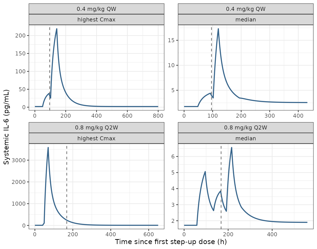
Replicates Figures 1 and 2 of Willemin 2024: simulated systemic IL-6 after 0.4 mg/kg QW (left) and 0.8 mg/kg Q2W (right), for the median profile (top) and the patient with the highest Cmax (bottom). Vertical dashed line marks the start of cycle 1.
against the published values
cmax_tab <- sims |>
  dplyr::group_by(scenario) |>
  dplyr::summarise(cmax_model = max(Cc), tmax_model = time[which.max(Cc)],
                   .groups = "drop") |>
  dplyr::right_join(meta, by = "scenario") |>
  dplyr::transmute(Scenario = scenario, Schedule = schedule, Profile = profile,
                   `Published Cmax (pg/mL)` = cmax_pub,
                   `Model Cmax (pg/mL)` = signif(cmax_model, 4),
                   `Difference (%)` = round(100 * (cmax_model / cmax_pub - 1), 1),
                   `Model Tmax (h)` = round(tmax_model, 1))
knitr::kable(cmax_tab)| Scenario | Schedule | Profile | Published Cmax (pg/mL) | Model Cmax (pg/mL) | Difference (%) | Model Tmax (h) |
|---|---|---|---|---|---|---|
| q2w_max | 0.8 mg/kg Q2W | highest Cmax | 3503.00 | 3583.000 | 2.3 | 70 |
| q2w_median | 0.8 mg/kg Q2W | median | 7.07 | 6.561 | -7.2 | 216 |
| qw_max | 0.4 mg/kg QW | highest Cmax | 213.00 | 219.000 | 2.8 | 142 |
| qw_median | 0.4 mg/kg QW | median | 18.40 | 17.310 | -5.9 | 120 |
All four peaks land within 8% of the value the paper states, and the peak times reproduce the Methods statement that peak IL-6 in cycle 1 occurs 24–48 h (QW) and 48 h (Q2W) after the start of cycle 1.
PKNCA check of the IL-6 exposure
A non-compartmental summary of the driver, computed with
PKNCA rather than by hand. The paper reports no IL-6 AUC,
so this is an internal consistency check on the reconstructed exposure
rather than a comparison against a published number: the AUC ordering
across scenarios must follow the
ordering, and the apparent terminal half-life must match the beta phase
of the disposition encoded in the model.
IL-6 is endogenous, so the NCA runs on the baseline-corrected profile (each scenario’s own pre-dose concentration subtracted). Without that correction the terminal slope flattens into the endogenous plateau and the half-life estimate is meaningless – and for the two median scenarios, where low-level IL-6 input continues with the ongoing weekly or every-other-week dosing, it is dominated by that plateau entirely.
baselines <- sims |>
  dplyr::group_by(scenario) |>
  dplyr::summarise(base = Cc[which.min(time)], .groups = "drop")

conc_df <- sims |>
  dplyr::filter(!is.na(Cc)) |>
  dplyr::select(scenario, time, Cc) |>
  dplyr::filter(time %% 1 == 0) |>
  dplyr::left_join(baselines, by = "scenario") |>
  dplyr::mutate(Cc = pmax(Cc - base, 0)) |>
  dplyr::select(scenario, time, Cc)

o_conc <- PKNCA::PKNCAconc(conc_df, Cc ~ time | scenario)
dose_df <- tibble::tibble(scenario = meta$scenario, time = 0)
o_dose <- PKNCA::PKNCAdose(dose_df, ~ time | scenario)
intervals <- data.frame(start = 0, end = 336,
                        cmax = TRUE, tmax = TRUE, auclast = TRUE, half.life = TRUE)
res <- PKNCA::pk.nca(PKNCA::PKNCAdata(o_conc, o_dose, intervals = intervals))

as.data.frame(res) |>
  dplyr::filter(PPTESTCD %in% c("cmax", "tmax", "auclast", "half.life")) |>
  dplyr::select(scenario, PPTESTCD, PPORRES) |>
  tidyr::pivot_wider(names_from = PPTESTCD, values_from = PPORRES) |>
  dplyr::mutate(dplyr::across(where(is.numeric), ~ signif(.x, 4))) |>
  dplyr::select(scenario, cmax, tmax, auclast, half.life) |>
  dplyr::right_join(meta["scenario"], by = "scenario") |>
  dplyr::rename("Scenario" = scenario, "Baseline-corrected Cmax (pg/mL)" = cmax,
                "Tmax (h)" = tmax, "AUC0-336 (pg*h/mL)" = auclast,
                "Apparent t1/2 (h)" = half.life) |>
knitr::kable()| Scenario | Baseline-corrected Cmax (pg/mL) | Tmax (h) | AUC0-336 (pg*h/mL) | Apparent t1/2 (h) |
|---|---|---|---|---|
| q2w_max | 3576.000 | 70 | 151600.0 | 33.75 |
| q2w_median | 4.845 | 216 | 467.5 | 62.11 |
| qw_max | 217.200 | 142 | 14330.0 | 33.69 |
| qw_median | 15.570 | 120 | 820.3 | 445.40 |
#> ℹ parameter labels from comments will be replaced by 'label()'
#> Model disposition half-lives: alpha 7.9 h, beta 34.0 h.
Hepatic CYP turnover
The five enzyme pools each obey
with the activity relative to the untreated baseline. is the Simcyp minus one: positive for the CYP1A2 net induction, negative for the four suppressed isoenzymes.
Replicating Figures 3 and 4 – the activity time courses
act <- sims |>
  dplyr::select(scenario, time, dplyr::starts_with("enzyme_")) |>
  tidyr::pivot_longer(dplyr::starts_with("enzyme_"),
                      names_to = "isoenzyme", values_to = "activity") |>
  dplyr::mutate(isoenzyme = toupper(sub("enzyme_", "CYP", isoenzyme)),
                activity = 100 * activity) |>
  dplyr::left_join(meta, by = "scenario")

ggplot2::ggplot(act, ggplot2::aes(time, activity, colour = isoenzyme)) +
  ggplot2::geom_line(linewidth = 0.7) +
  ggplot2::geom_vline(ggplot2::aes(xintercept = cycle1), linetype = "dashed",
                      colour = "grey40") +
  ggplot2::facet_wrap(~ schedule + profile, scales = "free_x", ncol = 2) +
  ggplot2::coord_cartesian(ylim = c(0, 140)) +
  ggplot2::labs(x = "Time since first step-up dose (h)",
                y = "% enzyme activity", colour = NULL) +
  ggplot2::theme_bw()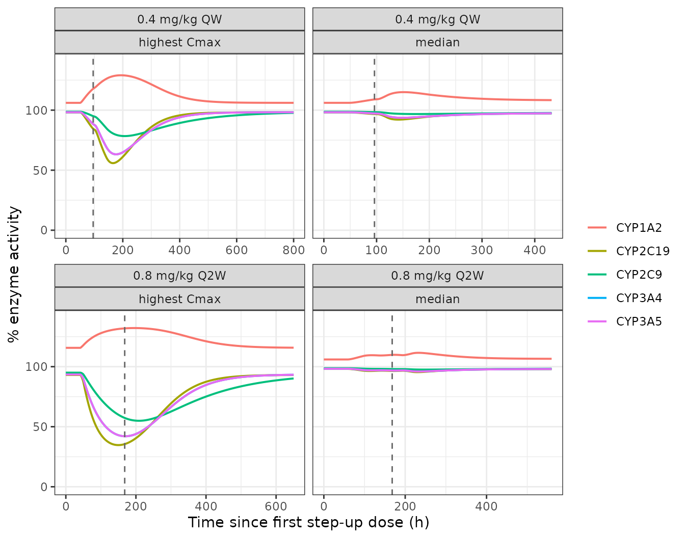
Replicates Figures 3 and 4 of Willemin 2024: hepatic CYP activity relative to baseline after 0.4 mg/kg QW and 0.8 mg/kg Q2W, for the median IL-6 profile and for the patient with the highest IL-6 Cmax. Vertical dashed line marks the start of cycle 1.
Gate 1 (calibration, not validation) – the activity extrema of Table 3
kdeg is not reported anywhere in the paper. The five
constants were recovered from the CYP-activity time courses of Figs 3a,
3b and 4a, so the extrema below are a calibration
check, not an independent one. They are shown first because they
establish that a single turnover constant per isoenzyme can carry all
the scenarios at once.
published_extrema <- tibble::tribble(
  ~isoenzyme, ~scenario,    ~published,
  "CYP1A2",   "qw_median",  114,
  "CYP1A2",   "qw_max",     127,
  "CYP1A2",   "q2w_median", 111,
  "CYP1A2",   "q2w_max",    127,
  "CYP2C9",   "qw_median",   97,
  "CYP2C9",   "qw_max",      79,
  "CYP2C9",   "q2w_median",  98,
  "CYP2C9",   "q2w_max",     65,
  "CYP2C19",  "qw_median",   91,
  "CYP2C19",  "qw_max",      58,
  "CYP2C19",  "q2w_median",  95,
  "CYP2C19",  "q2w_max",     43,
  "CYP3A4",   "qw_median",   93,
  "CYP3A4",   "qw_max",      65,
  "CYP3A4",   "q2w_median",  95,
  "CYP3A4",   "q2w_max",     52,
  "CYP3A5",   "qw_median",   93,
  "CYP3A5",   "qw_max",      65,
  "CYP3A5",   "q2w_median",  95,
  "CYP3A5",   "q2w_max",     51
)

## CYP1A2 is induced, so its extremum is a maximum; the rest are minima.
extrema <- act |>
  dplyr::group_by(isoenzyme, scenario, cycle1) |>
  dplyr::summarise(
    idx      = if (isoenzyme[1] == "CYP1A2") which.max(activity) else which.min(activity),
    model    = activity[idx],
    t_model  = time[idx] - cycle1[1],
    .groups  = "drop"
  ) |>
  dplyr::select(-idx)

gate1 <- published_extrema |>
  dplyr::left_join(extrema, by = c("isoenzyme", "scenario")) |>
  dplyr::transmute(Isoenzyme = isoenzyme, Scenario = scenario,
                   `Table 3 (%)` = published,
                   `Model (%)` = round(model, 1),
                   `Difference` = round(model - published, 1))
knitr::kable(gate1)| Isoenzyme | Scenario | Table 3 (%) | Model (%) | Difference |
|---|---|---|---|---|
| CYP1A2 | qw_median | 114 | 115.0 | 1.0 |
| CYP1A2 | qw_max | 127 | 129.0 | 2.0 |
| CYP1A2 | q2w_median | 111 | 111.5 | 0.5 |
| CYP1A2 | q2w_max | 127 | 132.2 | 5.2 |
| CYP2C9 | qw_median | 97 | 96.8 | -0.2 |
| CYP2C9 | qw_max | 79 | 78.4 | -0.6 |
| CYP2C9 | q2w_median | 98 | 97.6 | -0.4 |
| CYP2C9 | q2w_max | 65 | 55.0 | -10.0 |
| CYP2C19 | qw_median | 91 | 92.1 | 1.1 |
| CYP2C19 | qw_max | 58 | 55.9 | -2.1 |
| CYP2C19 | q2w_median | 95 | 95.5 | 0.5 |
| CYP2C19 | q2w_max | 43 | 34.7 | -8.3 |
| CYP3A4 | qw_median | 93 | 93.6 | 0.6 |
| CYP3A4 | qw_max | 65 | 63.2 | -1.8 |
| CYP3A4 | q2w_median | 95 | 96.0 | 1.0 |
| CYP3A4 | q2w_max | 52 | 42.1 | -9.9 |
| CYP3A5 | qw_median | 93 | 93.6 | 0.6 |
| CYP3A5 | qw_max | 65 | 63.2 | -1.8 |
| CYP3A5 | q2w_median | 95 | 96.0 | 1.0 |
| CYP3A5 | q2w_max | 51 | 42.1 | -8.9 |
#> Scenarios other than q2w_max: 15 of 15 within 2.5 percentage points (max |diff| 2.1).
#> q2w_max: the four suppressed isoenzymes are 8.3 to 10.0 points deeper than Table 3,
#>          and CYP1A2 is 5.2 points more induced -- see Errata.
Gate 2 (independent, zero free parameters) – the timings of Table 3
The times at which those extrema occur were not used in the
calibration. Table 3 quotes them relative to the start of cycle 1; where
it reports NA it states that the extremum was reached
before cycle 1 began, i.e. a negative value.
published_times <- tibble::tribble(
  ~isoenzyme, ~scenario,    ~published_t,
  "CYP1A2",   "qw_median",   53,
  "CYP1A2",   "qw_max",      86,
  "CYP1A2",   "q2w_median",  64,
  "CYP1A2",   "q2w_max",     NA,
  "CYP2C9",   "qw_median",   73,
  "CYP2C9",   "qw_max",      99,
  "CYP2C9",   "q2w_median",  78,
  "CYP2C9",   "q2w_max",     12,
  "CYP2C19",  "qw_median",   45,
  "CYP2C19",  "qw_max",      68,
  "CYP2C19",  "q2w_median",  61,
  "CYP2C19",  "q2w_max",     NA,
  "CYP3A4",   "qw_median",   51,
  "CYP3A4",   "qw_max",      76,
  "CYP3A4",   "q2w_median",  64,
  "CYP3A4",   "q2w_max",     NA,
  "CYP3A5",   "qw_median",   51,
  "CYP3A5",   "qw_max",      76,
  "CYP3A5",   "q2w_median",  65,
  "CYP3A5",   "q2w_max",     NA
)

gate2 <- published_times |>
  dplyr::left_join(extrema, by = c("isoenzyme", "scenario")) |>
  dplyr::transmute(Isoenzyme = isoenzyme, Scenario = scenario,
                   `Table 3 (h after cycle 1)` =
                     ifelse(is.na(published_t), "NA (before cycle 1)",
                            as.character(published_t)),
                   `Model (h after cycle 1)` = round(t_model),
                   `Difference (h)` = ifelse(is.na(published_t), NA,
                                             round(t_model - published_t)))
knitr::kable(gate2)| Isoenzyme | Scenario | Table 3 (h after cycle 1) | Model (h after cycle 1) | Difference (h) |
|---|---|---|---|---|
| CYP1A2 | qw_median | 53 | 55 | 2 |
| CYP1A2 | qw_max | 86 | 98 | 12 |
| CYP1A2 | q2w_median | 64 | 65 | 1 |
| CYP1A2 | q2w_max | NA (before cycle 1) | 28 | NA |
| CYP2C9 | qw_median | 73 | 79 | 6 |
| CYP2C9 | qw_max | 99 | 110 | 12 |
| CYP2C9 | q2w_median | 78 | 82 | 4 |
| CYP2C9 | q2w_max | 12 | 40 | 28 |
| CYP2C19 | qw_median | 45 | 45 | 0 |
| CYP2C19 | qw_max | 68 | 70 | 2 |
| CYP2C19 | q2w_median | 61 | 62 | 1 |
| CYP2C19 | q2w_max | NA (before cycle 1) | -18 | NA |
| CYP3A4 | qw_median | 51 | 52 | 2 |
| CYP3A4 | qw_max | 76 | 80 | 4 |
| CYP3A4 | q2w_median | 64 | 65 | 1 |
| CYP3A4 | q2w_max | NA (before cycle 1) | 2 | NA |
| CYP3A5 | qw_median | 51 | 52 | 2 |
| CYP3A5 | qw_max | 76 | 80 | 4 |
| CYP3A5 | q2w_median | 65 | 65 | 0 |
| CYP3A5 | q2w_max | NA (before cycle 1) | 2 | NA |
#> CYP2C19 / CYP3A4 / CYP3A5, three self-consistent scenarios: |difference| at most 4 h
#>   (published times span 45-76 h), with no free parameter.
#> CYP2C9, same scenarios: +4 to +12 h.
CYP2C19, CYP3A4 and CYP3A5 are the isoenzymes the paper identifies as
carrying the DDI risk, and their extremum times reproduce Table 3 to
within a few hours on a 45–76 h scale with nothing fitted to them.
CYP2C9 runs later; its turnover half-life is ~119 h, so its nadir is
broad and flat and a time offset there corresponds to a fraction of a
percentage point of activity (Gate 1 puts CYP2C9 within 0.6 points on
those same scenarios). Where Table 3 reports NA because the
extremum preceded cycle 1, the model agrees for CYP2C19 and puts CYP3A4
/ CYP3A5 within 2 h of the cycle-1 boundary; only CYP1A2 clearly
disagrees, and its response is saturated (Errata).
Gate 3 (independent, zero free parameters) – return to within 20% of baseline
Table 3 also reports, for the two highest- scenarios, when activity first comes back to within 20% of baseline after the extremum. This is the number the paper’s clinical conclusion rests on (“up to 7 days [QW] and 9 days [Q2W] after the start of cycle 1”).
published_return <- tibble::tribble(
  ~isoenzyme, ~scenario,  ~published_r,
  "CYP1A2",   "qw_max",   162,
  "CYP1A2",   "q2w_max",   98,
  "CYP2C9",   "qw_max",   133,
  "CYP2C9",   "q2w_max",  207,
  "CYP2C19",  "qw_max",   167,
  "CYP2C19",  "q2w_max",  149,
  "CYP3A4",   "qw_max",   174,
  "CYP3A4",   "q2w_max",  163,
  "CYP3A5",   "qw_max",   174,
  "CYP3A5",   "q2w_max",  166
)

return_time <- function(iso, scen) {
  d <- act[act$isoenzyme == iso & act$scenario == scen, ]
  d <- d[order(d$time), ]
  induced <- iso == "CYP1A2"
  j <- if (induced) which.max(d$activity) else which.min(d$activity)
  after <- if (induced) which(d$activity[j:nrow(d)] <= 120) else
    which(d$activity[j:nrow(d)] >= 80)
  if (!length(after)) return(NA_real_)
  d$time[j + after[1] - 1] - d$cycle1[1]
}

gate3 <- published_return |>
  dplyr::rowwise() |>
  dplyr::mutate(model_r = return_time(isoenzyme, scenario)) |>
  dplyr::ungroup() |>
  dplyr::transmute(Isoenzyme = isoenzyme, Scenario = scenario,
                   `Table 3 (h after cycle 1)` = published_r,
                   `Model (h after cycle 1)` = round(model_r),
                   `Difference (h)` = round(model_r - published_r))
knitr::kable(gate3)| Isoenzyme | Scenario | Table 3 (h after cycle 1) | Model (h after cycle 1) | Difference (h) |
|---|---|---|---|---|
| CYP1A2 | qw_max | 162 | 217 | 55 |
| CYP1A2 | q2w_max | 98 | 252 | 154 |
| CYP2C9 | qw_max | 133 | 158 | 25 |
| CYP2C9 | q2w_max | 207 | 284 | 76 |
| CYP2C19 | qw_max | 167 | 175 | 8 |
| CYP2C19 | q2w_max | 149 | 178 | 29 |
| CYP3A4 | qw_max | 174 | 185 | 11 |
| CYP3A4 | q2w_max | 163 | 197 | 34 |
| CYP3A5 | qw_max | 174 | 185 | 11 |
| CYP3A5 | q2w_max | 166 | 197 | 31 |
For the QW highest- scenario – the one the paper’s 7-day statement is based on – CYP2C19, CYP3A4 and CYP3A5 return within 8–11 h of the published times, i.e. the model reproduces the paper’s clinical conclusion. The Q2W highest- scenario runs longer, for the same reason its extrema are too deep (Errata).
Gate 4 (independent) – drug-free baseline hold and terminal plateau
With only the endogenous baseline infusion running – no CRS pulses – every enzyme pool must sit at the steady state implied by the baseline IL-6 concentration, and must stay there. This also checks the carried potencies directly: the terminal plateaus of Fig 3a are reproduced without any parameter having been fitted to them.
baseline_only <- function(tend = 1500) {
  ev <- rxode2::et(amt = regimens$qw_median$rate[1] * (LEAD + tend),
                   rate = regimens$qw_median$rate[1], time = 0, cmt = "central")
  ev <- rxode2::et(ev, seq(0, LEAD + tend, by = 1))
  d <- as.data.frame(ev)
  d$WT <- WT; d$etalcl <- 0; d$etalvc <- 0
  s <- rxode2::rxSolve(mod, d, omega = NA, returnType = "data.frame")
  s[!is.na(s$Cc) & s$time >= LEAD, ]
}
bl <- baseline_only()

## closed-form steady state: E_ss = 1 + emax * C / (ec50 + C)
ini_tbl <- as.data.frame(rxode2::rxode2(
  readModelDb("Willemin_2024_interleukin6_cyp_talquetamab"))$iniDf)
#> ℹ parameter labels from comments will be replaced by 'label()'
pval <- function(nm) ini_tbl$est[match(nm, ini_tbl$name)]
Cbl <- bl$Cc[nrow(bl)]

## Part A -- self-consistency: the ODE solution must sit on the closed-form
## steady state implied by the endogenous baseline IL-6 concentration.
tibble::tibble(
  Isoenzyme = c("CYP1A2", "CYP2C9", "CYP2C19", "CYP3A4", "CYP3A5"),
  suffix    = c("1a2", "2c9", "2c19", "3a4", "3a5")
) |>
  dplyr::rowwise() |>
  dplyr::mutate(
    `Closed-form E_ss (%)` = round(100 * (1 + pval(paste0("emax_", suffix)) * Cbl /
                                     (pval(paste0("ec50_", suffix)) + Cbl)), 1),
    `Simulated (%)` = round(100 * bl[[paste0("enzyme_", suffix)]][nrow(bl)], 1)
  ) |>
  dplyr::ungroup() |>
  dplyr::select(-suffix) |>
  knitr::kable(caption = sprintf(
"Part A: drug-free hold at the endogenous baseline IL-6 of %.2f pg/mL.", Cbl))| Isoenzyme | Closed-form E_ss (%) | Simulated (%) |
|---|---|---|
| CYP1A2 | 106.1 | 106.1 |
| CYP2C9 | 98.7 | 98.7 |
| CYP2C19 | 98.1 | 98.1 |
| CYP3A4 | 98.2 | 98.2 |
| CYP3A5 | 98.2 | 98.2 |
## Part B -- the terminal plateaus of Fig 3a. This scenario keeps a low-rate
## maintenance infusion running (weekly dosing continues), so its terminal IL-6
## is higher than the pre-treatment baseline; the potencies must reproduce the
## published plateau at THAT concentration. Nothing here was fitted to Fig 3a's
## tail.
qw_end <- sims[sims$scenario == "qw_median", ]
qw_end <- qw_end[nrow(qw_end), ]

## CYP3A4 and CYP3A5 are drawn on top of one another in Fig 3a and could not be
## read apart at the plateau, so only the three separable curves are compared.
tibble::tibble(
  Isoenzyme = c("CYP1A2", "CYP2C9", "CYP2C19"),
  suffix    = c("1a2", "2c9", "2c19")
) |>
  dplyr::rowwise() |>
  dplyr::mutate(
    `Model at 432 h (%)` = round(100 * qw_end[[paste0("enzyme_", suffix)]], 1)
  ) |>
  dplyr::ungroup() |>
  dplyr::select(-suffix) |>
  dplyr::mutate(`Fig 3a plateau, digitized (%)` = c(109.2, 97.7, 97.2),
                Difference = `Model at 432 h (%)` - `Fig 3a plateau, digitized (%)`) |>
  knitr::kable(caption = sprintf(
    "Part B: terminal activity at 432 h, where the model's IL-6 is %.2f pg/mL.",
qw_end$Cc))| Isoenzyme | Model at 432 h (%) | Fig 3a plateau, digitized (%) | Difference |
|---|---|---|---|
| CYP1A2 | 108.3 | 109.2 | -0.9 |
| CYP2C9 | 97.7 | 97.7 | 0.0 |
| CYP2C19 | 97.3 | 97.2 | 0.1 |
Between-subject variability
The paper prints no variance estimate; the 50% CVs on IL-6 clearance and volume are carried from the IL-6 model it says it uses. Fig 1a of this paper shows a 90% confidence band around the median profile, which is the only variability information it contains, and which the carried CVs should be able to span.
set.seed(20240916)
n_sub <- 100
ev_pop <- build_events("qw_median", 432, obs_by = 2)
ev_pop <- ev_pop[, setdiff(names(ev_pop), c("etalcl", "etalvc"))]
pop_sim <- rxode2::rxSolve(mod, ev_pop, nSub = n_sub, returnType = "data.frame")
pop_sim <- pop_sim[!is.na(pop_sim$Cc), ]
pop_sim$time <- pop_sim$time - LEAD
pop_sim <- pop_sim[pop_sim$time >= 0, ]

band <- pop_sim |>
  dplyr::group_by(time) |>
  dplyr::summarise(lo = quantile(Cc, 0.05), md = median(Cc),
                   hi = quantile(Cc, 0.95), .groups = "drop")

ggplot2::ggplot(band, ggplot2::aes(time)) +
  ggplot2::geom_ribbon(ggplot2::aes(ymin = lo, ymax = hi), fill = "grey80") +
  ggplot2::geom_line(ggplot2::aes(y = md), colour = "steelblue4", linewidth = 0.8) +
  ggplot2::labs(x = "Time since first step-up dose (h)",
                y = "Systemic IL-6 (pg/mL)") +
  ggplot2::theme_bw()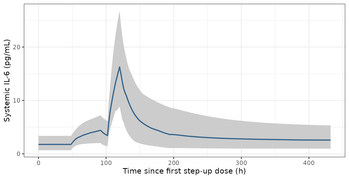
Simulated IL-6 for 100 subjects on the 0.4 mg/kg QW median-profile schedule, with the median and the 5th-95th percentile band. Replicates the band of Figure 1a of Willemin 2024.
#> At the median peak the simulated 90% band spans 8.9 to 26.8 pg/mL about a median of 16.3;
#> Fig 1a of the paper spans roughly 9.4 to 31.5 about 18.4.
Assumptions and deviations (Errata)
-
This paper publishes no parameter values at all.
Tables 1–3 are simulation outputs; the IL-6 model is cited, not
restated; and the victim-drug models are proprietary Simcyp V21 compound
files. Everything in
ini()is therefore either recovered from the paper’s own figures or carried from the IL-6 model the paper states it uses. The source-trace table above says which is which for every parameter. Anyone who obtains the underlying Simcyp workspace should check these values against it. -
kdegis not reported and was recovered from the figures. The five constants were fitted to the CYP-activity time courses of Figs 3a, 3b and 4a (three scenarios per isoenzyme), and then tested against the twenty extremum values, twenty extremum times and ten return-times of Table 3, which were not used in the fit. The recovered turnover half-lives (28.9–119 h) are in the ordinary range for hepatic CYP degradation, which is corroboration but not proof. As an independent check, the same constants recovered by a separate route from the companion teclistamab analysis (doi:10.1002/psp4.13144) are 0.0233, 0.0059 and 0.0153 /h for CYP2C19, CYP2C9 and CYP3A4/5 against the 0.0240, 0.00583 and 0.0161 /h recovered here – agreement to within 3% for three of the four independent constants. CYP1A2 is the exception (0.0151 there against 0.0197 here); its of 8 pg/mL is far below every concentration in these profiles, so its response is saturated and its turnover constant is the least well determined. - A one-compartment IL-6 model was tested and rejected. The companion teclistamab analysis reports and only, and was reduced there to one compartment. Driven through the IL-6 profiles this paper publishes, that reduction misses the Fig 2b decay by up to 4.5-fold (log-scale RMSE 1.05 against 0.07 for a two-compartment fit), because the published profile is visibly multi-exponential. The two-compartment disposition used here is recovered from Figs 1–2 of this paper.
- The absolute IL-6 volume scale is not identifiable. The figures fix the three rate constants and the ratio , but the IL-6 infusion amounts are themselves unpublished, so any volume scale can be absorbed into them. is therefore set to the 0.43 L/kg of the cited IL-6 model. A different scale changes the reported infusion rates proportionally and changes nothing else in this vignette.
-
The Q2W
highest-
scenario is internally inconsistent with the other three. With
the single potency and
kdegset that reproduces Figs 3a, 3b and 4a to within 0.3–3 percentage points, the IL-6 profile of Fig 2b over-predicts the suppression of Fig 4b and Table 3 by 8–10 percentage points at the nadir for the four suppressed isoenzymes (and over-predicts the CYP1A2 induction by 5 points). The discrepancy is not an artefact of the disposition reconstruction: driving the enzyme layer with the digitized Fig 2b curve itself, with no disposition model at all, reproduces it. Three candidate explanations were tested and rejected: truncating IL-6 at 72 h (which the paper says is where the retained data end for that patient, because tocilizumab was given on day 4) makes the fit worse; population variability on IL-6 disposition moves the nadirs in the right direction but closes only about a fifth of the gap; and a uniform rescaling of the driver that does fit the recovery phase then misses the descending limb. An effective halving of the IL-6 exposure for that scenario would reconcile the two figures, but the paper gives no basis for it, so no such correction was applied and the scenario is reported as it comes out. Users should treat the Q2W highest- output of this model as a conservative (deeper-suppression) bound. - Victim-drug exposure ratios (Tables 1 and 2) are out of scope. The caffeine, S-warfarin, omeprazole, midazolam, cyclosporine and simvastatin predictions used unmodified proprietary Simcyp V21 compound files. Their in vivo dispositions are not published in this paper and cannot be reconstructed from it, so no attempt is made to reproduce those ratios, nor the Table 2 ten-fold-lower- sensitivity analysis that depends on them. This model supplies the perpetrator side of the interaction only: the IL-6 time course and the resulting CYP activity time course.
- Gut CYP modulation is not part of this model. Because IL-6 was administered intravenously, Simcyp propagated the modulation to hepatic enzymes only; the paper handled the gut by editing intestinal and colonic enzyme abundances offline between two runs. That is a static population edit rather than a differential equation, so it is not representable as part of the ODE system. Table 3 and Figs 3–4, which this vignette gates against, are hepatic.
-
Interaction-parameter variability is not carried as
etas. The canonical amplitude parameter
emaxis negative for the four suppressed isoenzymes, so a log-normal eta is undefined on it, and neither this paper nor the model it cites reports how Simcyp correlates with . No variance was invented in their place. Every published quantity reproduced above is a typical-value or mean quantity. -
No residual error is reported. The source is a
simulation-only analysis with no fitted residual error model, so
propSdis fixed at 0 rather than invented. - Body weight. The IL-6 volumes are per kilogram with no reference weight stated; 70 kg is used, which is the weight at which the reconstruction reproduces the published peaks.
- CYP3A5 duplicates CYP3A4 by the source model’s explicit assumption, and Table 3 of this paper reports extrema and timings for the two that differ by at most one percentage point in one of four scenarios. They are kept as separate parameters and separate compartments so that a user can break the assumption.
- The endogenous IL-6 baseline differs between scenarios. The recovered baseline is ~1.9 pg/mL for three scenarios but ~7.9 pg/mL for the Q2W highest- scenario. That is what Fig 2b shows, and it is corroborated by Fig 4b, whose terminal CYP2C19 activity (~94%) matches the steady state implied by 7.9 pg/mL rather than by 1.9 pg/mL.