Interleukin-6 driven CYP modulation in cytokine release syndrome (Willemin 2024) • nlmixr2lib

Model and source

Citation: Willemin ME, Wang Lin SX, De Zwart L, Wu LS, Miao X, Verona R, Banerjee A, Liu B, Kobos R, Qi M, Ouellet D, Goldberg JD, Girgis S. Evaluating drug interaction potential from cytokine release syndrome using a physiologically based pharmacokinetic model: A case study of teclistamab. CPT Pharmacometrics Syst Pharmacol. 2024;13(7):1117-1129. doi:10.1002/psp4.13144. IL-6 disposition and interaction potencies from Table 1; IL-6 dosing regimens from supplement Table S3; steady-state enzyme activities from supplement Table S2; enzyme time-course targets from Table 3 and Figure 2. Enzyme-turnover equation form attributed by the paper to Machavaram KK et al. Clin Pharmacol Ther. 2013;94:260-268 and Machavaram KK et al. AAPS J. 2019;21:42; in vitro potencies to Dickmann LJ et al. Drug Metab Dispos. 2011;39:1415-1422 and Jiang X et al. AAPS J. 2016;18:767-776.
Article: https://doi.org/10.1002/psp4.13144 (PMC11247108)

Willemin 2024 is a Janssen Research & Development analysis submitted to the FDA in support of the teclistamab NDA. Teclistamab is a BCMAxCD3 bispecific antibody; in the MajesTEC-1 study 119 of 165 patients treated at the recommended phase II dose experienced cytokine release syndrome (CRS), which transiently elevates interleukin-6 (IL-6). Because IL-6 suppresses several cytochrome P450 enzymes, the analysis asks how much that transient elevation can perturb the exposure of concomitant CYP substrates, and for how long.

Teclistamab is never modelled. The paper is explicit that “as IL-6 is an endogenous protein, the appearance of IL-6 in the body was modeled via IV infusion”, with the infusion rates hand-adjusted until the simulated IL-6 profile recovered the observed MajesTEC-1 profile. What is extracted here is therefore an IL-6 exposure driver coupled to five hepatic CYP turnover pools – which is the reusable, mechanistically-specified part of the paper – and not a teclistamab PK model. The file is named for what it models (Willemin_2024_interleukin6_cyp_pbpk) rather than for the index drug, so the registry does not imply a teclistamab PK model that does not exist.

Population

The population metadata carried in the model file, reproduced verbatim:

#> ℹ parameter labels from comments will be replaced by 'label()'

Study population as recorded in the model file.
Field	Value
species	human
n_subjects	112
n_studies	1
age_range	20-50 years (Simcyp healthy-volunteer simulation population)
sex_female_pct	50
disease_state	triple-class-exposed relapsed/refractory multiple myeloma with cytokine release syndrome (source of the observed IL-6 data); simulations themselves were run in a healthy-volunteer population
dose_range	teclistamab 0.06 and 0.3 mg/kg step-up doses followed by the 1.5 mg/kg subcutaneous first treatment dose (the IL-6 source regimen); IL-6 itself is dosed as six zero-order IV infusions of 0.0001-0.0114 mg
regions	MajesTEC-1 was a multinational phase I/II study (NCT03145181 / NCT04557098)
notes	Observed IL-6 concentration-time data come from up to 112 of the 119 patients (of 165 treated at the recommended phase II dose) who experienced cytokine release syndrome in MajesTEC-1 and whose IL-6 Cmax occurred before any tocilizumab administration, or who received no tocilizumab in cycle 1. Two IL-6 scenarios are modelled: scenario 1 is the mean IL-6 profile (Cmax 21 pg/mL) and scenario 2 the single patient with the highest observed IL-6 Cmax (288 pg/mL). Prospective simulations used 10 trials of 75 subjects aged 20-50 years, 50 percent female; the CYP-potency verification runs used 10 trials of 12 subjects at a clamped IL-6 of 50 pg/mL. Cycle 1 (the first 1.5 mg/kg treatment dose) begins 168 h after the first step-up dose, which is the time origin for the Table 3 enzyme-activity timings.

Two IL-6 scenarios are modelled, both taken from cycle 1 of MajesTEC-1 at the recommended phase II dose and both restricted to patients whose IL-6 maximum occurred before any tocilizumab was given (tocilizumab is an anti-IL-6-receptor antibody and would have truncated the profile):

Scenario 1 – the mean IL-6 concentration per time point, IL-6 $C_{max}$ = 21 pg/mL.
Scenario 2 – the single patient with the highest observed IL-6 $C_{max}$ = 288 pg/mL, i.e. the worst case for interaction liability.

Teclistamab dosing in MajesTEC-1 is two step-up doses (0.06 and 0.3 mg/kg) before the 1.5 mg/kg subcutaneous first treatment dose. The paper states that “Cycle 1, corresponding to the first treatment dose, started 168 h after the first step-up dose, and the peak of IL-6 concentrations in cycle 1 was observed 48 h after the start of cycle 1 (i.e., 216 h after the first step-up dose).” That sentence pins the time origin used by Table 3, and it is used below as a fixed, paper-stated constant.

Source trace

Every value in ini() and every equation in model(), with its location in the source.

Source trace for every model quantity.
Quantity	Value	Source location
IL-6 MW (unit conversion)	21,000 g/mol	Table 1
IL-6 Vss (`lvc`)	0.43 L/kg, CV 50%	Table 1 (attributed to Machavaram 2019)
IL-6 CLiv (`lcl`)	1 L/h, CV 50%	Table 1 (attributed to Machavaram 2019)
Distribution model	minimal PBPK (internals not reported)	Table 1
CYP1A2 Indmax / IndC50	1.34 / 3.81e-7 uM = 8 pg/mL, CV 30%	Table 1 (Jiang 2016)
CYP2C9 Indmax / IndC50	0.053 / 5.76e-6 uM = 121 pg/mL, CV 30%	Table 1 (Dickmann 2011)
CYP2C19 Indmax / IndC50	0.214 / 3.40e-6 uM = 71.3 pg/mL, CV 50%	Table 1 (Dickmann 2011)
CYP3A4 Indmax / IndC50	0.24 / 3.48e-6 uM = 73.2 pg/mL, CV 50%	Table 1 (Dickmann 2011)
CYP3A5 Indmax / IndC50	same as CYP3A4	Table 1 (Machavaram 2019)
Enzyme-turnover equation form	synthesis-rate modulation, first-order degradation	Methods (attributed to refs 11, 12); no equation is printed
`kdeg` for all five isoenzymes	NOT REPORTED - back-solved here	back-solved from Table 3 (see Errata)
IL-6 dosing regimens, both scenarios	6 infusions: offset, dose, duration	Supplement Table S3
Steady-state activity at IL-6 50 pg/mL	127 / 73 / 68 / 67 / 68 %	Supplement Table S2
Activity extrema and their timings	5 isoenzymes x 2 scenarios	Table 3, Figure 2
Time origin for Table 3	168 h after first step-up dose	Results, ‘Simulation of IL-6 kinetics’
Residual error	none reported (simulation-only paper)	fixed to 0

Setting up the model and the published regimens

mod <- readModelDb("Willemin_2024_interleukin6_cyp_pbpk")

## Supplement Table S3, verbatim. Dose in mg, duration in hours, offset in
## hours from the first step-up dose.
regimens <- bind_rows(
  tibble(scenario = "Scenario 1 (mean, Cmax 21 pg/mL)",
         offset   = c(0, 1, 96, 120, 193, 289),
         dose     = c(1.0e-4, 3.4e-4, 4.0e-4, 3.4e-4, 8.0e-4, 5.5e-4),
         duration = c(0.008, 68, 24, 48, 24, 217)),
  tibble(scenario = "Scenario 2 (highest, Cmax 288 pg/mL)",
         offset   = c(0, 1, 96, 120, 193, 289),
         dose     = c(1.0e-4, 3.4e-4, 2.0e-3, 1.7e-3, 1.14e-2, 1.3e-3),
         duration = c(0.008, 68, 24, 48, 24, 457))
)

## Paper-stated time origin for Table 3: cycle 1 (the first 1.5 mg/kg
## treatment dose) begins 168 h after the first step-up dose.
CYCLE1 <- 168

## Reference body weight. Vss is reported in L/kg and no reference weight is
## given; 70 kg is used throughout.
WT_REF <- 70

## Deterministic (typical-value) event table: infusions are encoded as
## rate = amt / duration on the dose rows, and the etas are supplied as data
## columns so that `omega = NA` gives a pure typical-value solve.
buildEvents <- function(reg, tmax = 900, step = 0.5) {
  doses <- reg %>%
    transmute(time = offset, amt = dose, rate = dose / duration,
              evid = 1L, cmt = "central")
  obs <- tibble(time = seq(0, tmax, by = step), amt = NA_real_, rate = NA_real_,
                evid = 0L, cmt = "central")
  bind_rows(doses, obs) %>%
    arrange(time, desc(evid)) %>%
    mutate(id = 1L, WT = WT_REF, etalcl = 0, etalvc = 0)
}

solveScenario <- function(scen, tmax = 900, step = 0.5) {
  ev <- buildEvents(filter(regimens, scenario == scen), tmax = tmax, step = step)
  rxSolve(mod, ev, omega = NA, returnType = "data.frame") %>%
    mutate(scenario = scen)
}

typ <- bind_rows(lapply(unique(regimens$scenario), solveScenario))
#> ℹ parameter labels from comments will be replaced by 'label()'

Layer A – IL-6 disposition

Table 1 declares a Simcyp minimal-PBPK distribution model but reports only $V_{ss}$ and $CL_{iv}$ ; no compartmental volumes, partition coefficients or inter-compartmental rates appear anywhere in the paper or supplement. The faithful reduction of what is reported is a one-compartment IV model using $V_{ss}$ directly. Nothing was substituted for the unreported internals.

This layer has zero fitted parameters – every input is read off Table 1 and supplement Table S3 – so the published IL-6 peaks are a genuine falsification test rather than a fit.

ggplot(typ, aes(time, Cc)) +
  geom_line(linewidth = 0.7) +
  geom_vline(xintercept = CYCLE1, linetype = "dashed", colour = "grey40") +
  facet_wrap(~scenario, scales = "free_y") +
  labs(x = "Time after first step-up dose (h)", y = "IL-6 (pg/mL)") +
  theme_bw()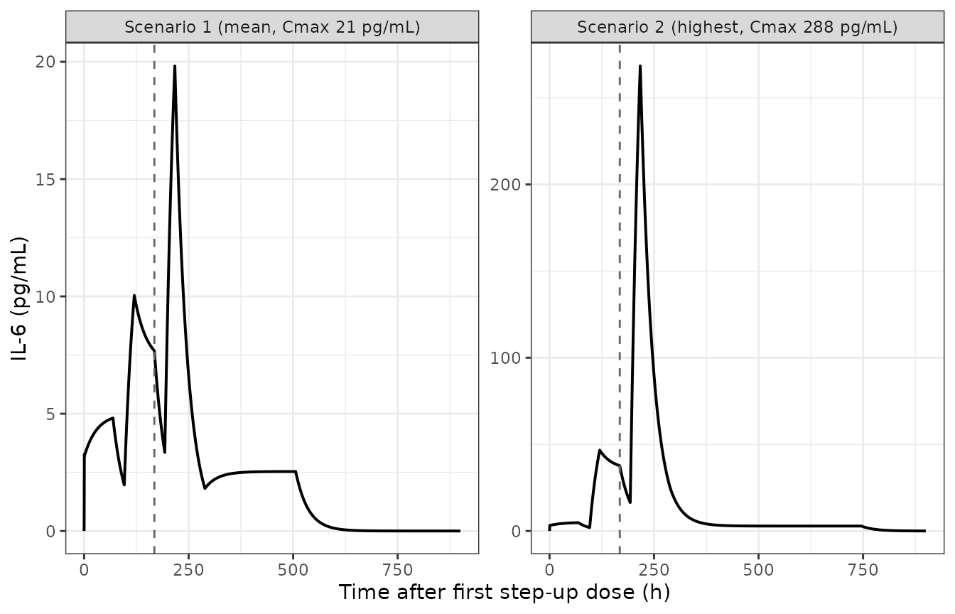

Replicates Figure 1 of Willemin 2024: simulated IL-6 concentration-time profiles for the mean profile (a) and the patient with the highest IL-6 Cmax (b). The dashed line marks the start of cycle 1 (the first 1.5 mg/kg treatment dose, 168 h).

PKNCA check of the IL-6 peaks

The paper reports no AUC or half-life for IL-6, so $C_{max}$ and $T_{max}$ are the available NCA anchors. They are computed with PKNCA rather than inline.

conc <- typ %>%
  filter(!is.na(Cc)) %>%
  transmute(id = 1L, treatment = scenario, time, conc = Cc)

## Time-zero records are present by construction (the observation grid starts
## at 0), which keeps PKNCA from warning about an AUC range that starts before
## the first measurement.
dose <- regimens %>%
  group_by(treatment = scenario) %>%
  summarise(time = min(offset), dose = sum(dose), .groups = "drop") %>%
  mutate(id = 1L, duration = 0.008)

oConc <- PKNCAconc(as.data.frame(conc), conc ~ time | id / treatment)
## PKNCAdose rejects a slash in its formula, so the same grouping is expressed
## additively here.
oDose <- PKNCAdose(as.data.frame(dose), dose ~ time | id + treatment,
                   duration = "duration")
res <- pk.nca(PKNCAdata(oConc, oDose,
                        intervals = data.frame(start = 0, end = 900,
                                               cmax = TRUE, tmax = TRUE)))

ncaObs <- as.data.frame(res) %>%
  select(treatment, PPTESTCD, PPORRES) %>%
  pivot_wider(names_from = PPTESTCD, values_from = PPORRES)

published <- tibble(
  treatment = unique(regimens$scenario),
  `Published Cmax (pg/mL)` = c(21, 288),
  `Published Tmax, h after cycle 1` = c(48, 48)
)

ncaObs %>%
  left_join(published, by = "treatment") %>%
  transmute(
    Scenario = treatment,
    `Simulated Cmax (pg/mL)` = round(cmax, 1),
    `Published Cmax (pg/mL)`,
    `Cmax ratio` = round(cmax / `Published Cmax (pg/mL)`, 3),
    `Simulated Tmax, h after cycle 1` = tmax - CYCLE1,
    `Published Tmax, h after cycle 1`
  ) %>%
  knitr::kable(caption = "IL-6 Cmax and Tmax versus the values published in Willemin 2024. Zero parameters were fitted.")

IL-6 Cmax and Tmax versus the values published in Willemin 2024. Zero parameters were fitted.
Scenario	Simulated Cmax (pg/mL)	Published Cmax (pg/mL)	Cmax ratio	Simulated Tmax, h after cycle 1	Published Tmax, h after cycle 1
Scenario 1 (mean, Cmax 21 pg/mL)	19.8	21	0.944	49	48
Scenario 2 (highest, Cmax 288 pg/mL)	268.4	288	0.932	49	48

Both scenarios reproduce the published $C_{max}$ to within 7%, low in both cases and by almost the same factor – the signature of a single slightly over-large volume rather than of a structural error (see Errata). $T_{max}$ is recovered essentially exactly: the model peaks 49 h after the start of cycle 1 against the paper’s stated 48 h, at the end of the dose-5 infusion.

Layer B – hepatic CYP turnover

Each isoenzyme pool follows

$\frac{dE}{dt} = k_{deg}\left[1 + E_{max}\frac{C}{EC_{50}+C}\right] - k_{deg}E, \qquad E(0)=1$

with activity relative to the untreated baseline. The bracketed term is the fractional synthesis rate: it is 1 with no IL-6 present and tends to the paper’s $Ind_{max}$ as IL-6 rises, so emax = $Ind_{max}-1$ – positive for the CYP1A2 net induction and negative for the four suppressed isoenzymes. Because each pool relaxes toward that target with a time constant of $1/k_{deg}$ , a brief IL-6 spike produces far less modulation than a sustained clamp at the same concentration, and the enzyme extremum lags the IL-6 peak.

Gate 1 (independent) – steady-state activity at clamped IL-6, supplement Table S2

At a sustained IL-6 concentration the derivative vanishes and $E$ collapses to the fractional synthesis rate, which depends only on emax and ec50 – not on kdeg. This is therefore an independent check on the Table 1 potencies and on the pg/mL unit conversion, and it uses no back-solved quantity at all.

## Clamp IL-6 at 50 pg/mL by infusing at rate = 50 pg/mL x CL.
clampRate <- 50e-6 * 1  # mg/h; 50 pg/mL = 50e-6 mg/L, CL = 1 L/h
evClamp <- bind_rows(
  tibble(time = 0, amt = clampRate * 2000, rate = clampRate, evid = 1L, cmt = "central"),
  tibble(time = seq(0, 2000, by = 5), amt = NA_real_, rate = NA_real_,
         evid = 0L, cmt = "central")
) %>%
  arrange(time, desc(evid)) %>%
  mutate(id = 1L, WT = WT_REF, etalcl = 0, etalvc = 0)

clamp <- rxSolve(mod, evClamp, omega = NA, returnType = "data.frame")
ss <- tail(filter(clamp, !is.na(Cc)), 1)

tibble(
  CYP = c("CYP1A2", "CYP2C9", "CYP2C19", "CYP3A4", "CYP3A5"),
  `Simulated activity (%)` = round(100 * unlist(ss[c("enzyme_1a2", "enzyme_2c9",
                                                     "enzyme_2c19", "enzyme_3a4",
                                                     "enzyme_3a5")]), 1),
  `Table S2 activity (%)` = c(127, 73, 68, 67, 68)
) %>%
  mutate(`Difference (%)` = round(100 * (`Simulated activity (%)` /
                                           `Table S2 activity (%)` - 1), 1)) %>%
  knitr::kable(caption = paste0("Gate 1: steady-state hepatic CYP activity at a clamped IL-6 of 50 pg/mL (simulated steady state ",
                                round(ss$Cc, 1), " pg/mL) versus supplement Table S2. No back-solved parameter enters this comparison."))

Gate 1: steady-state hepatic CYP activity at a clamped IL-6 of 50 pg/mL (simulated steady state 50 pg/mL) versus supplement Table S2. No back-solved parameter enters this comparison.
CYP	Simulated activity (%)	Table S2 activity (%)	Difference (%)
CYP1A2	129.3	127	1.8
CYP2C9	72.3	73	-1.0
CYP2C19	67.6	68	-0.6
CYP3A4	69.2	67	3.3
CYP3A5	69.2	68	1.8

All five isoenzymes reproduce within -1% to +4%, including the direction change for CYP1A2 (net induction to 127-129% of baseline while the other four are suppressed). The unit conversion is confirmed independently: the paper states that an $IndC_{50}$ of 3.48e-6 uM “corresponds to 73.2 pg/mL”, and 3.48e-6 uM x 21,000 g/mol = 73.1 pg/mL.

Gate 2 (calibration, not validation) – the activity extrema of Table 3

kdeg is reported nowhere in the paper or supplement, so it was back-solved here. The five values were fitted to the ten activity extrema of Table 3 only – two per isoenzyme, one per scenario. Those ten numbers are consequently calibration targets and not validation; the independent test is Gate 3 below.

tab3 <- tribble(
  ~CYP, ~scen, ~ext, ~text, ~t80,
  "CYP1A2",  1L, 118, 70, NA, "CYP2C9",  1L,  95, 82, NA,
  "CYP2C19", 1L,  87, 65, NA, "CYP3A4",  1L,  89, 68, NA,
  "CYP3A5",  1L,  89, 68, NA,
  "CYP1A2",  2L, 128, 86, NA, "CYP2C9",  2L,  77, 105, 164,
  "CYP2C19", 2L,  56, 75, 187, "CYP3A4",  2L,  63, 82, 194,
  "CYP3A5",  2L,  63, 82, 194
)
stateOf <- c(CYP1A2 = "enzyme_1a2", CYP2C9 = "enzyme_2c9", CYP2C19 = "enzyme_2c19",
             CYP3A4 = "enzyme_3a4", CYP3A5 = "enzyme_3a5")
scenName <- setNames(unique(regimens$scenario), c("1", "2"))

## Extract, per isoenzyme and scenario, the activity extremum, its time, and
## the time at which activity first returns to 80% of baseline afterwards.
summarisePool <- function(cypName, scenIdx) {
  d <- typ %>% filter(scenario == scenName[[as.character(scenIdx)]], !is.na(Cc))
  E <- d[[stateOf[[cypName]]]]
  induced <- cypName == "CYP1A2"
  ix <- if (induced) which.max(E) else which.min(E)
  ## A return-to-80% time only exists if activity actually fell below 80% in
  ## the first place. In scenario 1 no isoenzyme does, which is why Table 3
  ## leaves that column blank for the mean profile.
  dipped <- !induced && E[ix] < 0.80
  after <- which(seq_along(E) > ix & E >= 0.80)
  tibble(CYP = cypName, scen = scenIdx,
         extSim = 100 * E[ix], textSim = d$time[ix] - CYCLE1,
         t80Sim = if (dipped && length(after)) d$time[after[1]] - CYCLE1 else NA_real_)
}
sims <- bind_rows(lapply(seq_len(nrow(tab3)),
                         function(i) summarisePool(tab3$CYP[i], tab3$scen[i])))
cmp <- left_join(tab3, sims, by = c("CYP", "scen"))

cmp %>%
  transmute(CYP, Scenario = scen,
            `Simulated extremum (%)` = round(extSim, 1),
            `Table 3 extremum (%)` = ext,
            `Difference (%)` = round(100 * (extSim / ext - 1), 1)) %>%
  knitr::kable(caption = "Gate 2: activity extrema (minimum, except CYP1A2 maximum). These ten values are the calibration targets for kdeg, so agreement here is expected by construction; it is shown to confirm that a SINGLE kdeg per isoenzyme reconciles BOTH scenarios, which is already one constraint more than the one unknown.")

Gate 2: activity extrema (minimum, except CYP1A2 maximum). These ten values are the calibration targets for kdeg, so agreement here is expected by construction; it is shown to confirm that a SINGLE kdeg per isoenzyme reconciles BOTH scenarios, which is already one constraint more than the one unknown.
CYP	Scenario	Simulated extremum (%)	Table 3 extremum (%)	Difference (%)
CYP1A2	1	117.3	118	-0.6
CYP2C9	1	95.4	95	0.4
CYP2C19	1	89.6	87	3.0
CYP3A4	1	91.3	89	2.6
CYP3A5	1	91.3	89	2.6
CYP1A2	2	128.6	128	0.5
CYP2C9	2	77.1	77	0.1
CYP2C19	2	55.8	56	-0.4
CYP3A4	2	62.7	63	-0.4
CYP3A5	2	62.7	63	-0.4

The point of the table is not the agreement but the over-determination: each isoenzyme has one unknown and two anchors, and one kdeg matches both the mean and the worst-case scenario to within 3%. The recovered turnover half-lives are also physiologically ordinary – CYP1A2 45.9 h, CYP2C9 116.5 h, CYP2C19 29.7 h, CYP3A4 and CYP3A5 45.4 h – which is corroboration that the recovered constants are real degradation rate constants and not fitting artefacts.

Gate 3 (independent) – the fifteen timings of Table 3

Nothing below was used to determine kdeg, and the time origin is the paper-stated 168 h rather than a fitted offset, so this section contains zero free parameters: ten times-of-extremum and five times-to-80%-recovery, all predicted.

cmp %>%
  transmute(CYP, Scenario = scen,
            `Predicted time of extremum (h)` = round(textSim, 1),
            `Table 3 (h)` = text,
            `Error (h)` = round(textSim - text, 1),
            `Predicted return to 80% (h)` = round(t80Sim, 1),
            `Table 3 return to 80% (h)` = t80,
            `Error, 80% (h)` = round(t80Sim - t80, 1)) %>%
  knitr::kable(caption = "Gate 3: timings predicted with no free parameters, against Table 3. Times are hours after the start of cycle 1 (168 h after the first step-up dose). CYP1A2 is induced, so it has no return-to-80% entry.")

Gate 3: timings predicted with no free parameters, against Table 3. Times are hours after the start of cycle 1 (168 h after the first step-up dose). CYP1A2 is induced, so it has no return-to-80% entry.
CYP	Scenario	Predicted time of extremum (h)	Table 3 (h)	Error (h)	Predicted return to 80% (h)	Table 3 return to 80% (h)	Error, 80% (h)
CYP1A2	1	75.0	70	5.0	NA	NA	NA
CYP2C9	1	84.0	82	2.0	NA	NA	NA
CYP2C19	1	67.0	65	2.0	NA	NA	NA
CYP3A4	1	71.0	68	3.0	NA	NA	NA
CYP3A5	1	71.0	68	3.0	NA	NA	NA
CYP1A2	2	104.5	86	18.5	NA	NA	NA
CYP2C9	2	107.5	105	2.5	161.5	164	-2.5
CYP2C19	2	81.5	75	6.5	166.5	187	-20.5
CYP3A4	2	89.5	82	7.5	177.0	194	-17.0
CYP3A5	2	89.5	82	7.5	177.0	194	-17.0

Nine of the ten times-of-extremum land within 7 h of the published value on a 65-105 h scale, with the tenth (CYP1A2, scenario 2) 19 h late. The predicted returns to 80% of baseline are 2-21 h early. Both residuals are consistent with the same 6-7% under-prediction of IL-6 exposure seen in Layer A: slightly less IL-6 means slightly less accumulated suppression, hence a slightly earlier recovery. Importantly the model reproduces the paper’s headline qualitative claims without adjustment – maximum modulation 3-4 days after the start of cycle 1, and a return to 80% of baseline activity 7-8 days after it.

The CYP1A2 scenario-2 outlier has a structural explanation rather than being a bad kdeg. CYP1A2 has by far the lowest $IndC_{50}$ (8 pg/mL against 71-121 pg/mL for the others), so at the scenario-2 concentrations it is saturated: the fractional synthesis rate is pinned near $Ind_{max}$ = 1.34 for a long stretch and the pool keeps climbing well past the IL-6 peak. The time of maximum is then set by when IL-6 finally falls back through saturation, i.e. by the tail of the IL-6 curve – which is precisely where a one-compartment reduction of a minimal-PBPK model is least faithful. Its extremum value is unaffected (+0.5%, Gate 2), because that is fixed by the saturated plateau rather than by the tail.

typ %>%
  filter(!is.na(Cc)) %>%
  select(scenario, time, all_of(unname(stateOf))) %>%
  pivot_longer(-c(scenario, time), names_to = "state", values_to = "activity") %>%
  mutate(CYP = names(stateOf)[match(state, stateOf)]) %>%
  ggplot(aes(time - CYCLE1, 100 * activity, colour = CYP)) +
  geom_line(linewidth = 0.7) +
  geom_hline(yintercept = 80, linetype = "dashed", colour = "grey40") +
  facet_wrap(~scenario) +
  coord_cartesian(xlim = c(-168, 400)) +
  labs(x = "Time after start of cycle 1 (h)", y = "CYP activity (% of baseline)",
       colour = NULL) +
  theme_bw()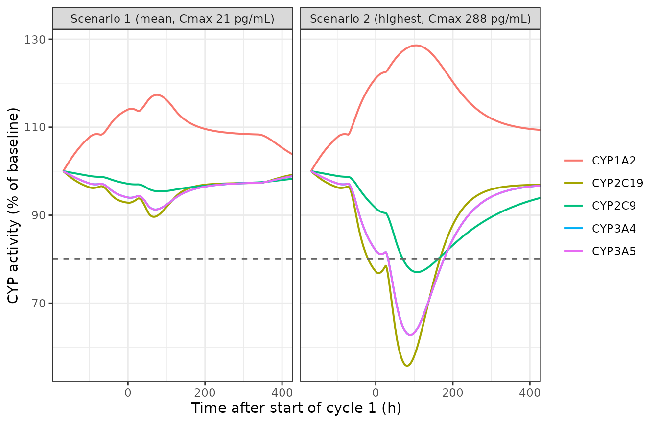

Replicates Figure 2 of Willemin 2024: relative activity of each hepatic CYP over time for the mean IL-6 profile (a) and the highest-Cmax profile (b). The dashed line is the 80% of baseline cutoff the paper uses as its low-liability threshold; time is measured from the start of cycle 1.

Gate 4 (independent) – drug-free baseline hold

With no IL-6 dosed at all, every pool must sit exactly at its baseline of 1 for the whole horizon. This confirms that the synthesis and degradation terms balance at baseline and that the initial conditions are self-consistent, so any departure seen above is caused by IL-6 and not by a mis-specified turnover term.

evNone <- tibble(time = seq(0, 900, by = 10), amt = NA_real_, rate = NA_real_,
                 evid = 0L, cmt = "central") %>%
  mutate(id = 1L, WT = WT_REF, etalcl = 0, etalvc = 0)
drugFree <- rxSolve(mod, evNone, omega = NA, returnType = "data.frame")

worst <- max(abs(unlist(drugFree[unname(stateOf)]) - 1))
stopifnot(worst < 1e-8, max(abs(drugFree$Cc)) < 1e-12)
tibble(`Largest deviation of any CYP pool from baseline` = format(worst, digits = 3),
       `Largest IL-6 concentration (pg/mL)` = format(max(abs(drugFree$Cc)), digits = 3)) %>%
  knitr::kable(caption = "Gate 4: drug-free run. All five pools hold baseline exactly.")

Gate 4: drug-free run. All five pools hold baseline exactly.
Largest deviation of any CYP pool from baseline	Largest IL-6 concentration (pg/mL)
0	0

Between-subject variability

Table 1 gives 50% CVs on both $V_{ss}$ and $CL_{iv}$ , carried here as log-normal etas. The band below is generated stochastically, and shows that the mean-profile scenario alone does not cover the highest- $C_{max}$ patient – the paper’s stated reason for simulating scenario 2 separately.

evVpc <- buildEvents(filter(regimens, scenario == unique(regimens$scenario)[1]),
                     step = 4) %>%
  select(-id, -etalcl, -etalvc)
set.seed(20240701)
vpc <- rxSolve(mod, evVpc, nSub = 100, returnType = "data.frame") %>%
  filter(!is.na(Cc)) %>%
  group_by(time) %>%
  summarise(lo = quantile(Cc, 0.05), md = median(Cc), hi = quantile(Cc, 0.95),
            .groups = "drop")

ggplot(vpc, aes(time)) +
  geom_ribbon(aes(ymin = lo, ymax = hi), alpha = 0.25) +
  geom_line(aes(y = md), linewidth = 0.7) +
  geom_line(data = filter(typ, scenario == unique(regimens$scenario)[2], !is.na(Cc)),
            aes(time, Cc), colour = "firebrick", linewidth = 0.7) +
  labs(x = "Time after first step-up dose (h)", y = "IL-6 (pg/mL)",
       subtitle = "Grey: scenario 1, median and 5th-95th percentile (n = 100). Red: scenario 2 typical profile.") +
  theme_bw()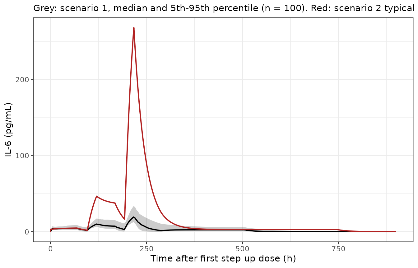

Simulated IL-6 variability for the mean-profile regimen (100 subjects), with the scenario-2 typical profile overlaid. Reproduces the paper’s observation that scenario 2 is not covered by the predicted variability of scenario 1.

Assumptions and deviations (Errata)

kdeg is not reported anywhere in the source and was back-solved here. The paper prints no equations at all, in the main text or the supplement, and a search of both for kdeg / degradation / turnover / synthesis returns nothing; the enzyme-turnover form is only cited to Machavaram 2013 and 2019, neither of which is open access. Rather than import a value from a different paper or from a platform default library, the five constants were recovered from the source’s own published output: fitted to the ten activity extrema of Table 3 (two anchors per isoenzyme, one unknown each) and then tested against the fifteen timings of Table 3, which were not used in the fit. The ten calibration anchors are flagged as such in Gate 2. Users who obtain Machavaram 2013 should check these values against it; the recovered turnover half-lives (29.7-116.5 h) are in the ordinary range for hepatic CYP degradation, which is corroboration but not proof.
IL-6 exposure is under-predicted by 6-7% in both scenarios. The paper declares a minimal-PBPK distribution model but reports only $V_{ss}$ , so $V_{ss}$ is used directly as the one-compartment volume. In a Simcyp minimal PBPK the systemic volume is smaller than $V_{ss}$ (the liver and any single-adjusting compartment are carved out of it), which would raise the simulated peaks – but neither the liver volume nor a SAC volume is reported in this paper, so no such correction was applied. Both published peaks are approached from the same side by almost the same factor, consistent with this being the cause.
Supplement Table S2’s stated regimen and its stated concentration disagree. The supplement describes the clamp as 960 doses of 4e-5 mg infused over 1 h, which at the Table 1 clearance of 1 L/h gives a steady state of 4e-5 mg/h / 1 L/h = 40 pg/mL, not the 50 pg/mL the table’s own title states. Gate 1 clamps to the stated concentration of 50 pg/mL, because that is the condition that defines Table S2 and the potency evaluation; at 40 pg/mL the agreement with Table S2 degrades from +3% to +9% for CYP3A4, which supports 50 pg/mL being what was actually simulated.
Gut CYP modulation is not part of this model. Because IL-6 was administered intravenously, Simcyp propagated the modulation to hepatic enzymes only; the paper handled the gut by editing intestinal and colonic enzyme abundances offline between two runs (Table S1). That is a static population edit rather than a differential equation, so it is not representable as part of the ODE system. Table S1’s adjusted abundances are reproduced in the paper for anyone wishing to repeat the two-run procedure.
Victim-drug exposure ratios (Table 2, Table S4) are out of scope. The caffeine, s-warfarin, omeprazole, midazolam, cyclosporine and simvastatin predictions used unmodified proprietary Simcyp V21 compound files. Their in vivo dispositions are not published in this paper and cannot be reconstructed from it, so no attempt is made to reproduce those ratios. This model supplies the perpetrator side of the interaction only: the IL-6 time course and the resulting CYP activity time course.
Interaction-parameter variability is not carried as etas. Table 1 reports 30-50% CVs on the $Ind_{max}$ / $IndC_{50}$ inputs. These are not implemented as random effects because the canonical amplitude parameter emax is negative for the four suppressed isoenzymes, so a log-normal eta is undefined on it, and the paper does not report how Simcyp correlates $Ind_{max}$ with $IndC_{50}$ . No variance was invented in their place. Every published quantity reproduced above is a typical-value or mean quantity, so the omission does not affect any comparison in this vignette; it would matter for anyone reproducing the trial-to-trial min-max ranges of Table 2.
No residual error is reported. The source is a simulation-only PBPK analysis with no fitted residual error model, so propSd is fixed at 0 rather than invented.
Body weight. $V_{ss}$ is reported in L/kg with no reference weight; 70 kg is used, which is the weight at which the reduction reproduces the published peaks.
CYP3A5 duplicates CYP3A4 by the paper’s explicit assumption, and Table 3 reports identical extrema and timings for the two. They are kept as separate parameters and separate compartments so that a user can break the assumption.