Magnesium bone implant PBPK (Ward 2026)
Source:vignettes/articles/Ward_2026_magnesium_pbpk.Rmd
Ward_2026_magnesium_pbpk.RmdModel and source
- Citation: Ward JP, Ahmed SK, Liu Y. Physiologically Based Pharmacokinetic Model of Magnesium Implant Absorption and Distribution in Tissue and Organs. ACS Omega. 2026 Jan 22;11(4):5144-5153. doi:10.1021/acsomega.5c06910. PMCID: PMC12878740. Parameter derivations and the full (8-ODE) pathway model are in Supporting Information A-C (ao5c06910_si_001.pdf).
- Description: PBPK (whole-body, 4-compartment linear ODE). Long-term magnesium (Mg(II)) homeostasis in an average healthy 70 kg adult perturbed by a biodegradable Mg (alloy) bone implant. Exchangeable (‘exposed’) Mg is tracked in blood serum, bone, bulk tissue (muscle + soft tissue + liver), and a local peri-implant tissue zone; Mg enters from diet (after intestinal absorption) and from constant-rate implant corrosion, and leaves by concentration-proportional urinary excretion. Deterministic: no IIV and no residual error are reported. Supports multiple/larger implants (n_implant) and dietary intake control (f_diet), and is used to predict the number of implants and the time scale required to reach hypermagnesemia.
- Article: https://doi.org/10.1021/acsomega.5c06910 (ACS Omega 2026;11(4):5144-5153, PMC12878740, open access)
- Supporting Information A-C:
ao5c06910_si_001.pdf, distributed with the article.
This is not a drug-disposition model. It is a deterministic, physiologically based description of whole-body magnesium (Mg(II)) homeostasis in an average healthy adult, perturbed by the slow corrosion of a biodegradable magnesium bone implant. There is no dose, no absorption phase and no residual error, so the validation below uses the endogenous / mechanistic patterns (steady-state hold, closed-form steady states, characteristic time scales, perturbation response) rather than non-compartmental analysis.
Population
The model is not fitted to an individual-level data set. Its parameters describe an “average” healthy 70 kg adult carrying about 1000.7 mmol of total body Mg, assembled from the physiology literature in Supporting Information B (Tables S2-S3): serum 3 L, red blood cells 2 L, bone 12.3 L and bulk soft tissue (muscle, soft tissue and liver, lumped) 52.7 L. The exchange clearances between blood and bone and between blood and tissue were then tuned so the model reproduces the stable-isotope Mg tracer kinetics of Sojka 1997 and Sabatier 2003 (Supporting Information B, Figure S2). The authors describe the resulting values as “representative rather than definitive”.
Reduced renal function is represented by lowering the urinary
excretion clearance cl_renal (the paper’s
gamma), with a matched reduction in rate_diet
so that pre-implant homeostasis Cse = rate_diet / cl_renal
is preserved; chronic renal failure is taken as roughly one third of the
healthy value (Section 2.2.3).
No long-term human validation data exist: the paper notes that no human study has monitored serum Mg over the 2-12 month window in which a Mg implant corrodes.
The same information is available programmatically via the model’s
population metadata
(readModelDb("Ward_2026_magnesium_pbpk")()$population –
readModelDb() returns the model function, so the
trailing () evaluates it to the model object).
mod <- rxode2::rxode2(readModelDb("Ward_2026_magnesium_pbpk"))

# Every published scenario is a change to one or more of the fixed ini()
# values, so scenarios are built by re-pinning them rather than by dosing.
solve_scenario <- function(times,
                           n_implant      = 1,
                           f_diet         = 1,
                           rate_diet      = 6,
                           cl_renal       = 10.9,
                           rate_implant   = 0.05,
                           v_implant_zone = 0.00527) {
  # Bind to distinct local names first: rxode2::ini() is non-standard-evaluating,
  # so `ini(n_implant = n_implant)` would resolve the right-hand side against the
  # model's own parameter rather than this function's argument.
  .n    <- n_implant
  .rho  <- f_diet
  .diet <- rate_diet
  .lgam <- log(cl_renal)
  .sig  <- rate_implant
  .vi   <- v_implant_zone
  m <- suppressMessages(
    mod |>
      rxode2::ini(n_implant      = .n) |>
      rxode2::ini(f_diet         = .rho) |>
      rxode2::ini(rate_diet      = .diet) |>
      rxode2::ini(lcl_renal      = .lgam) |>
      rxode2::ini(rate_implant   = .sig) |>
      rxode2::ini(v_implant_zone = .vi)
  )
  as.data.frame(rxode2::rxSolve(m, rxode2::et(times), atol = 1e-12, rtol = 1e-10))
}

# Log-spaced grid for the paper's log-x figures; fine linear grid for the
# time-constant checks.
t_log <- c(0, 10^seq(-3, 4, length.out = 500))
Source trace
Every ini() value carries an in-file comment pointing at
its source location in
inst/modeldb/endogenous/Ward_2026_magnesium_pbpk.R. They
are collected here for review. All parameter values come from
Table 1 (page 5145); the “source” column of that table
records whether each value was read from the literature, derived from
the Supporting Information B homeostasis ratios (H), derived from the
Table S2/S3 data (R), or is an estimate (I, V).
| File parameter | Paper symbol | Value | Units | Source location |
|---|---|---|---|---|
v_serum |
V_s |
3 | L | Table 1 |
v_rbc |
V_r |
2 | L | Table 1 |
v_bone |
V_N |
12.3 | L | Table 1 |
v_tissue |
V_Ttot |
52.7 | L | Table 1 |
v_implant_zone |
V_I |
0.00527 | L | Table 1; chosen so V_I / V_Ttot = 1e-4 (SI B, S15) |
lcl_renal |
gamma |
log(10.9) | log(L/day) | Table 1; = rate_diet / Cse (SI B, S11) |
q_serum_bone |
mu_1 |
6.05 | L/day | Table 1 |
q_bone_serum |
mu_-1 |
0.0775 | L/day | Table 1; fixed by mu_-1 / mu_1 = Cse / CNe (SI B,
S12) |
q_serum_tissue |
k_1 |
138 | L/day | Table 1 |
q_tissue_serum |
k_-1 |
34.7 | L/day | Table 1; fixed by k_-1 / k_1 = Cse / CTe (SI B,
S12) |
rate_diet |
phi_D |
6 | mmol/day | Table 1 |
rate_implant |
sigma |
0.05 | mmol/day | Table 1; one 3.2 x 32 mm screw |
f_exposed_bone |
phi |
0.3 | - | Table 1 |
kp_unexposed_serum |
xi_1 |
0.538 | - | Table 1 |
kp_rbc_serum |
xi_2 |
0.452 | - | Table 1 |
kp_unexposed_tissue |
xi_3 |
3.00 | - | Table 1 |
n_implant |
n |
1 | - | eq 9, Section 2.2.2 (scenario lever) |
f_diet |
rho |
1 | - | eq 10, Section 2.2.3 (scenario lever) |
| Model structure | Source location |
|---|---|
d/dt(serum) |
eq 1 (page 5146), with the rho dietary-control factor
of eq 10 (page 5149) |
d/dt(bone) |
eq 2 (page 5146) |
d/dt(other) |
eq 3 (page 5146) |
d/dt(implant_zone) |
eq 4 (page 5146) |
Initial conditions Cse, CNe,
CTe
|
eq 5 (page 5146) |
n implant scaling of V_I,
sigma, xi
|
eq 9 (page 5147) |
Total serum Cc = serum * (1 + xi_1)
|
Table 1, C_hom = Cse + Csu = 0.85 mmol/L
|
Compartment mapping
| Paper compartment | File compartment | Note |
|---|---|---|
Blood serum, C_s
|
serum |
exposed (exchangeable) Mg only |
Bone, C_N
|
bone |
|
Tissue, C_T
|
other |
muscle + soft tissue + liver, lumped |
Implant region, C_I
|
implant_zone |
localized peri-implant tissue |
The paper’s bulk tissue store T maps onto the nlmixr2lib
canonical lumped-remainder compartment other rather than a
compartment literally named tissue: the role is defined by
the lumping, and the paper never resolves muscle from liver from generic
soft tissue. implant_zone is a new canonical registered
with this extraction (see
inst/references/compartment-names.md).
Units and dimensional analysis
Unlike most nlmixr2lib models, the states here are concentrations (mmol/L), not amounts: the published system is written directly in concentration, with the compartment volume and its exposed/unexposed capacitance factor appearing as the divisor on the left-hand side. Every “exchange rate constant” in Table 1 has units of L/day, i.e. it is a volumetric clearance, not a first-order rate constant.
| ODE | Numerator units | Divisor units | Result |
|---|---|---|---|
serum |
mmol/day + (L/day)(mmol/L) = mmol/day |
v_serum*(1+xi_1) + v_rbc*xi_2 = L |
mmol/L/day |
bone |
(L/day)(mmol/L) = mmol/day |
phi*v_bone = L |
mmol/L/day |
other |
(L/day)(mmol/L) = mmol/day |
v_tissue*(1+xi_3) = L |
mmol/L/day |
implant_zone |
mmol/day + (L/day)(mmol/L) = mmol/day |
v_iz*(1+xi_3) = L |
mmol/L/day |
xi = V_I / V_Ttot and the four xi_j
partition ratios are dimensionless, as are n_implant and
f_diet. The observation
Cc = serum * (1 + xi_1) is total (exposed + unexposed)
serum Mg in mmol/L – the clinically measured quantity that the 0.65-1.05
mmol/L reference range and the 1.05 mmol/L hypermagnesemia threshold
refer to.
# Reference quantities used throughout, all from Table 1.
phiD  <- 6       # dietary intake rate, mmol/day
gam0  <- 10.9    # healthy urinary excretion clearance, L/day
k1    <- 138     # serum -> tissue exchange clearance, L/day
kn1   <- 34.7    # tissue -> serum
mu1   <- 6.05    # serum -> bone
mun1  <- 0.0775  # bone -> serum
VT    <- 52.7; VN <- 12.3; Vs <- 3; Vr <- 2
xi1   <- 0.538; xi2 <- 0.452; xi3 <- 3; phi_b <- 0.3
xi0   <- 0.00527 / VT      # V_I / V_Ttot for a single implant

Chom  <- 0.85              # Table 1, homeostatic total serum Mg (mmol/L)
Chyp  <- 1.05              # Table 1, hypermagnesemia threshold
Csev  <- 2.9               # Table 1, severe / "dangerous" concentration
Chyp_norm <- Chyp / Chom   # Table 2 footnote: C*_hyp = C_hyp / C_hom
Csev_norm <- Csev / Chom
c(Chyp_norm = Chyp_norm, Csev_norm = Csev_norm)  # paper: ~1.24 and ~3.41
#> Chyp_norm Csev_norm
#>  1.235294  3.411765
Steady-state hold (no implant)
With no implant the system must sit at the homeostasis of eq 5
forever. The initial conditions are computed inside model()
from rate_diet / cl_renal (eq 5) rather than from Table 1’s
rounded printed Cse = 0.553, so this check is exact rather
than merely close: gamma = 10.9 is itself the rounded form
of phiD / Cse, and seeding from the printed
Cse would leave the model 0.4% off its own steady
state.
Closed-form steady states (eq 8)
Equation 8 gives the exact long-term normalised steady states of eqs 1-4:
(Cs*, CN*, CT*, CI*) = (1 + sigma/phiD,  1 + sigma/phiD,  1 + sigma/phiD,
                        1 + sigma/phiD + sigma*gamma/(xi*k1*phiD))
so serum, bone and tissue all rise by the same proportion
sigma/phiD, and only the implant zone – which absorbs the
whole release term into a tiny volume – runs higher. This is the model’s
sharpest structural check: it pins rate_implant,
rate_diet, lcl_renal,
q_serum_tissue and the n scaling of eq 9
simultaneously.
eq8 <- function(n) {
  sig <- n * 0.05
  xi  <- n * xi0
  c(Cs = 1 + sig / phiD,
    CI = 1 + sig / phiD + sig * gam0 / (xi * k1 * phiD))
}

n_grid <- c(1, 2, 5, 10, 20, 30, 40)
eq8_chk <- lapply(n_grid, function(n) {
  s <- solve_scenario(times = t_log, n_implant = n)
  p <- eq8(n)
  tibble(
    n          = n,
    Cs_sim     = tail(s$Cs_norm, 1),  Cs_eq8 = unname(p["Cs"]),
    CN_sim     = tail(s$CN_norm, 1),
    CT_sim     = tail(s$CT_norm, 1),
    CI_sim     = tail(s$CI_norm, 1),  CI_eq8 = unname(p["CI"])
  )
}) |> bind_rows()

eq8_chk |>
  mutate(across(-n, ~ signif(.x, 6))) |>
  dplyr::rename(
    "n implants" = n,
    "Cs* (sim)" = Cs_sim, "Cs* (eq 8)" = Cs_eq8,
    "CN* (sim)" = CN_sim, "CT* (sim)" = CT_sim,
    "CI* (sim)" = CI_sim, "CI* (eq 8)" = CI_eq8
  ) |>
knitr::kable(caption = "Simulated long-term steady states vs the closed form of eq 8.")| n implants | Cs* (sim) | Cs* (eq 8) | CN* (sim) | CT* (sim) | CI* (sim) | CI* (eq 8) |
|---|---|---|---|---|---|---|
| 1 | 1.00833 | 1.00833 | 1.00833 | 1.00833 | 7.59046 | 7.59046 |
| 2 | 1.01667 | 1.01667 | 1.01667 | 1.01667 | 7.59879 | 7.59879 |
| 5 | 1.04167 | 1.04167 | 1.04167 | 1.04167 | 7.62379 | 7.62379 |
| 10 | 1.08333 | 1.08333 | 1.08333 | 1.08333 | 7.66546 | 7.66546 |
| 20 | 1.16667 | 1.16667 | 1.16667 | 1.16667 | 7.74879 | 7.74879 |
| 30 | 1.25000 | 1.25000 | 1.25000 | 1.25000 | 7.83213 | 7.83213 |
| 40 | 1.33333 | 1.33333 | 1.33333 | 1.33333 | 7.91546 | 7.91546 |
# Simulation and closed form agree to solver tolerance for every n, and the
# paper's statement that Cs*, CN* and CT* are indistinguishable holds exactly.
stopifnot(
  max(abs(eq8_chk$Cs_sim - eq8_chk$Cs_eq8)) < 1e-6,
  max(abs(eq8_chk$CI_sim - eq8_chk$CI_eq8)) < 1e-4,
  max(abs(eq8_chk$Cs_sim - eq8_chk$CN_sim)) < 1e-6,
  max(abs(eq8_chk$Cs_sim - eq8_chk$CT_sim)) < 1e-6
)
For a single screw this gives Cs* = 1.00833 – the
paper’s “the rest of the compartments eventually peaks at around 0.8%
above homeostatic levels” – and CI* = 7.59, matching Figure
2.
Figure 2 – a single Mg screw implant
# Replicates Figure 2 of Ward 2026: normalised concentrations over time for a
# single 3.2 x 32 mm screw releasing sigma = 0.05 mmol/day.
TMg_formula <- (1 / gam0) *
  ((1 + xi1) * Vs + xi2 * Vr + (mu1 / mun1) * phi_b * VN +
     (1 + xi3) * (k1 / kn1) * VT)

f2 <- solve_scenario(times = t_log, n_implant = 1) |>
  select(time, Cs_norm, CN_norm, CT_norm, CI_norm) |>
  pivot_longer(-time, names_to = "state", values_to = "value") |>
  mutate(state = recode(state,
                        Cs_norm = "Cs* (serum)", CN_norm = "CN* (bone)",
                        CT_norm = "CT* (tissue)", CI_norm = "CI* (implant zone)")) |>
  filter(time > 0)

ggplot(f2, aes(time, value, colour = state)) +
  geom_line(linewidth = 0.7) +
  geom_hline(yintercept = Chyp_norm, linetype = "dashed") +
  geom_hline(yintercept = Csev_norm, linetype = "dashed", colour = "red") +
  geom_vline(xintercept = TMg_formula, linetype = "dotted") +
  scale_x_log10(limits = c(1e-3, 1e4)) +
  labs(x = "Time (days)", y = "Normalised concentration (Cj*)", colour = NULL,
       title = "Figure 2 - single Mg screw implant",
       caption = paste("Replicates Figure 2 of Ward 2026. Dashed lines: C*hyp and C*sev.",
                       "Dotted vertical: t = T_Mg."))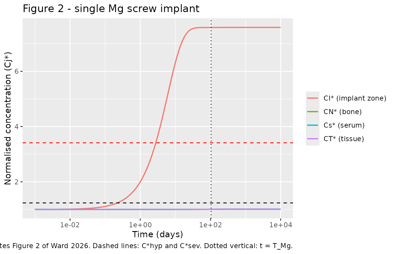
The implant zone reaches its elevated plateau of about 7.6 within roughly three weeks and stays there, above both the hypermagnesemia (1.24) and the “dangerous” (3.41) normalised thresholds, while serum, bone and tissue overlap each other and rise by less than 1%. That is the paper’s central conclusion for a single small implant: a large local effect and a negligible systemic one.
Figure 3 – multiple or larger implants
Equation 9 scales V_I, sigma and
xi together with the number of implants n, on
the assumption that the affected tissue regions do not overlap.
# Replicates Figure 3 of Ward 2026 (A: serum; B: implant zone).
f3 <- lapply(n_grid, function(n) {
  solve_scenario(times = t_log, n_implant = n) |>
    transmute(time, n = factor(n, levels = n_grid), Cs_norm, CI_norm)
}) |> bind_rows() |> filter(time > 0)

ggplot(filter(f3, time >= 1e-2), aes(time, Cs_norm, colour = n)) +
  geom_line(linewidth = 0.6) +
  geom_hline(yintercept = Chyp_norm, linetype = "dashed") +
  geom_vline(xintercept = TMg_formula, linetype = "dotted") +
  scale_x_log10(limits = c(1e-2, 1e4)) +
  labs(x = "Time (days)", y = "Cs* (normalised serum)", colour = "n implants",
       title = "Figure 3A - serum Mg for n implants",
       caption = "Replicates Figure 3A of Ward 2026. Dashed: C*hyp ~= 1.24.")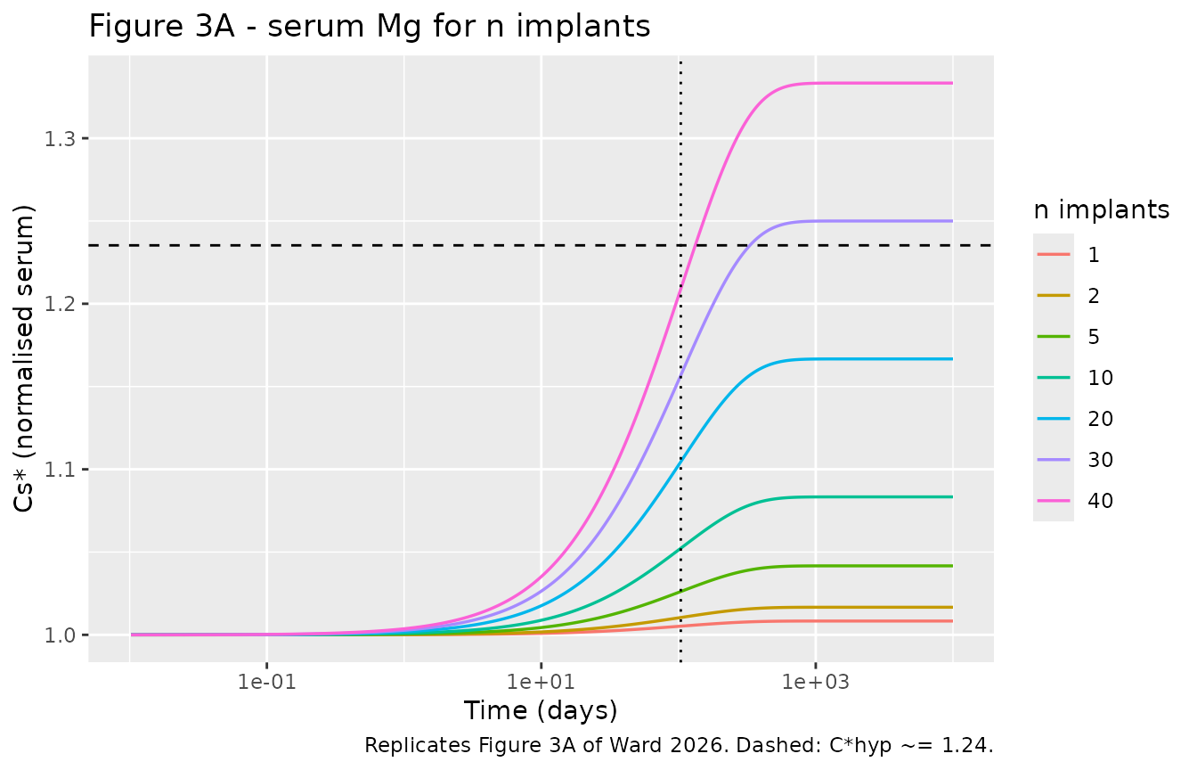
ggplot(f3, aes(time, CI_norm, colour = n)) +
  geom_line(linewidth = 0.6) +
  geom_hline(yintercept = Chyp_norm, linetype = "dashed") +
  geom_hline(yintercept = Csev_norm, linetype = "dashed", colour = "red") +
  scale_x_log10(limits = c(1e-3, 1e4)) +
  labs(x = "Time (days)", y = "CI* (normalised implant zone)", colour = "n implants",
       title = "Figure 3B - implant-zone Mg for n implants",
       caption = "Replicates Figure 3B of Ward 2026.")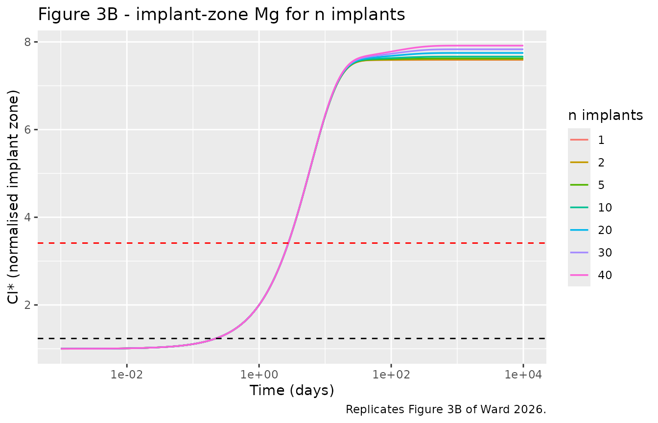
Figure 3B reproduces the paper’s observation that the implant-zone
curves are essentially independent of n for the first 2-3
days: eq 9 scales the release rate and the zone volume by the same
factor, so the local concentration is initially unaffected by how many
implants there are.
Characteristic time scales (Table 2)
Table 2 gives closed-form approximations for the two time constants,
defined as the time at which the change has completed a fraction
1 - exp(-1) = 0.632:
T_1  = V_T (1 + xi_3) / k_-1                                     ~= 6 days
T_Mg = (1/gamma) [ (1 + xi_1) V_s + xi_2 V_r
                   + (mu_1/mu_-1) phi V_N + (1 + xi_3)(k_1/k_-1) V_Ttot ]  ~= 104 days
t_fine <- seq(0, 1500, length.out = 150001)
s1     <- solve_scenario(times = t_fine, n_implant = 1)

# Time at which a monotone rise has completed 1 - exp(-1) of its total change.
t_632 <- function(x, tt) {
  target <- 1 + (tail(x, 1) - 1) * (1 - exp(-1))
  tt[which(x >= target)[1]]
}

T1_formula <- VT * (1 + xi3) / kn1
tab2 <- tibble(
  Quantity  = c("T_1 (implant zone)", "T_Mg (systemic)"),
  Simulated = c(t_632(s1$CI_norm, t_fine), t_632(s1$Cs_norm, t_fine)),
  Formula   = c(T1_formula, TMg_formula),
  Paper     = c(6, 104)
)
tab2 |>
  mutate(across(where(is.numeric), ~ signif(.x, 4))) |>
  dplyr::rename("Table 2 formula" = Formula, "Paper (rounded)" = Paper) |>
knitr::kable(caption = "Simulated time constants vs the Table 2 closed forms.")| Quantity | Simulated | Table 2 formula | Paper (rounded) |
|---|---|---|---|
| T_1 (implant zone) | 6.09 | 6.075 | 6 |
| T_Mg (systemic) | 105.20 | 103.800 | 104 |
# Both closed forms are asymptotic approximations in xi << 1, so a few percent
# of disagreement with the full four-ODE solve is expected and is the quantity
# actually being validated.
stopifnot(
  abs(tab2$Simulated[1] - tab2$Formula[1]) / tab2$Formula[1] < 0.05,
  abs(tab2$Simulated[2] - tab2$Formula[2]) / tab2$Formula[2] < 0.05,
  abs(tab2$Formula[1] - 6)   < 0.5,
  abs(tab2$Formula[2] - 104) < 2
)
The paper attributes “around 74%” of the systemic buildup time to
tissue and “about 25%” to bone; the four additive terms of
T_Mg reproduce that split directly.
TMg_terms <- c(
  serum  = (1 + xi1) * Vs,
  rbc    = xi2 * Vr,
  bone   = (mu1 / mun1) * phi_b * VN,
  tissue = (1 + xi3) * (k1 / kn1) * VT
)
round(100 * TMg_terms / sum(TMg_terms), 1)  # paper: tissue ~74%, bone ~25%
#>  serum    rbc   bone tissue
#>    0.4    0.1   25.4   74.1

stopifnot(
  abs(100 * TMg_terms[["tissue"]] / sum(TMg_terms) - 74) < 1.5,
  abs(100 * TMg_terms[["bone"]]   / sum(TMg_terms) - 25) < 1.5
)
Hypermagnesemia threshold – a binary answer key
Table 2 gives the critical release rate above which hypermagnesemia
is eventually reached, and Section 2.2.2 converts it to a number of
screws: sigma_hyp ~= 1.41 mmol/day, so
sigma_hyp / sigma_0 ~= 28-29 implants. That makes
n = 28 versus n = 29 a clean binary key which
pins rate_implant, rate_diet,
lcl_renal and the C_hyp / C_hom normalisation
all at once.
sigma_hyp <- function(n) phiD * (Chyp_norm - 1) / (1 - n * xi0)
sigma_hyp(28)   # paper: ~1.41 mmol/day
#> [1] 1.415729
sigma_hyp(28) / 0.05  # paper: minimum n is "28-29"
#> [1] 28.31457

thresh <- tibble(n = c(27, 28, 29, 30)) |>
  rowwise() |>
  mutate(Cs_star = tail(solve_scenario(times = t_log, n_implant = n)$Cs_norm, 1)) |>
  ungroup() |>
  mutate(hypermagnesemic = Cs_star > Chyp_norm)

thresh |>
  mutate(Cs_star = signif(Cs_star, 6)) |>
  dplyr::rename("n implants" = n, "Cs* (steady state)" = Cs_star,
                "Exceeds C*hyp" = hypermagnesemic) |>
  knitr::kable(caption = paste0("Hypermagnesemia threshold. C*hyp = 1.05/0.85 = ",
signif(Chyp_norm, 6), "."))| n implants | Cs* (steady state) | Exceeds C*hyp |
|---|---|---|
| 27 | 1.22500 | FALSE |
| 28 | 1.23333 | FALSE |
| 29 | 1.24167 | TRUE |
| 30 | 1.25000 | TRUE |
# The model crosses the threshold between 28 and 29 implants, exactly as
# reported. This is a strict binary assertion, not a tolerance band.
stopifnot(
  identical(thresh$hypermagnesemic, c(FALSE, FALSE, TRUE, TRUE)),
  abs(sigma_hyp(28) - 1.41) < 0.02
)
The onset time follows from Table 2’s
T_hyp = T_Mg log(sigma / (sigma - sigma_hyp)).
n_h    <- 40
sig_h  <- n_h * 0.05
Thyp_formula <- TMg_formula * log(sig_h / (sig_h - sigma_hyp(n_h)))

s40  <- solve_scenario(times = seq(0, 600, length.out = 60001), n_implant = n_h)
Thyp_sim <- seq(0, 600, length.out = 60001)[which(s40$Cs_norm >= Chyp_norm)[1]]

c(simulated = Thyp_sim, formula = Thyp_formula)  # both a few months, per Figure 6
#> simulated   formula
#>  132.4200  128.0894

# T_hyp is a T_Mg-based asymptotic approximation, so agreement to a few percent
# is the expected result.
stopifnot(abs(Thyp_sim - Thyp_formula) / Thyp_formula < 0.06)
Figure 4 – the scaled-up Sato plate
Sato et al. inserted a 30 x 10 x 1 mm Mg alloy plate in a rat. Scaled
up to human proportions (about 200 times in volume) this becomes a plate
of roughly 424 x 141 x 1 mm releasing sigma = 10 mmol/day,
with an affected tissue volume of V_I = 1.2 L
(xi ~= 0.023).
# Replicates Figure 4 of Ward 2026: the scaled-up Sato plate.
f4 <- solve_scenario(times = t_log, n_implant = 1,
                     rate_implant = 10, v_implant_zone = 1.2)

xi_plate <- 1.2 / VT
sato_eq8 <- c(Cs = 1 + 10 / phiD,
              CI = 1 + 10 / phiD + 10 * gam0 / (xi_plate * k1 * phiD))
c(Cs_sim = tail(f4$Cs_norm, 1), Cs_eq8 = unname(sato_eq8["Cs"]),
  CI_sim = tail(f4$CI_norm, 1), CI_eq8 = unname(sato_eq8["CI"]))
#>   Cs_sim   Cs_eq8   CI_sim   CI_eq8
#> 2.666667 2.666667 8.447967 8.447967

stopifnot(
  abs(tail(f4$Cs_norm, 1) - sato_eq8[["Cs"]]) < 1e-6,
  abs(tail(f4$CI_norm, 1) - sato_eq8[["CI"]]) < 1e-4
)

f4 |>
  select(time, Cs_norm, CN_norm, CT_norm, CI_norm) |>
  pivot_longer(-time, names_to = "state", values_to = "value") |>
  mutate(state = recode(state,
                        Cs_norm = "Cs* (serum)", CN_norm = "CN* (bone)",
                        CT_norm = "CT* (tissue)", CI_norm = "CI* (implant zone)")) |>
  filter(time > 0) |>
  ggplot(aes(time, value, colour = state)) +
  geom_line(linewidth = 0.7) +
  geom_hline(yintercept = Chyp_norm, linetype = "dashed") +
  geom_hline(yintercept = Csev_norm, linetype = "dashed", colour = "red") +
  geom_vline(xintercept = TMg_formula, linetype = "dotted") +
  scale_x_log10(limits = c(1e-3, 1e4)) +
  labs(x = "Time (days)", y = "Normalised concentration (Cj*)", colour = NULL,
       title = "Figure 4 - scaled-up Sato plate (sigma = 10 mmol/day)",
       caption = "Replicates Figure 4 of Ward 2026.")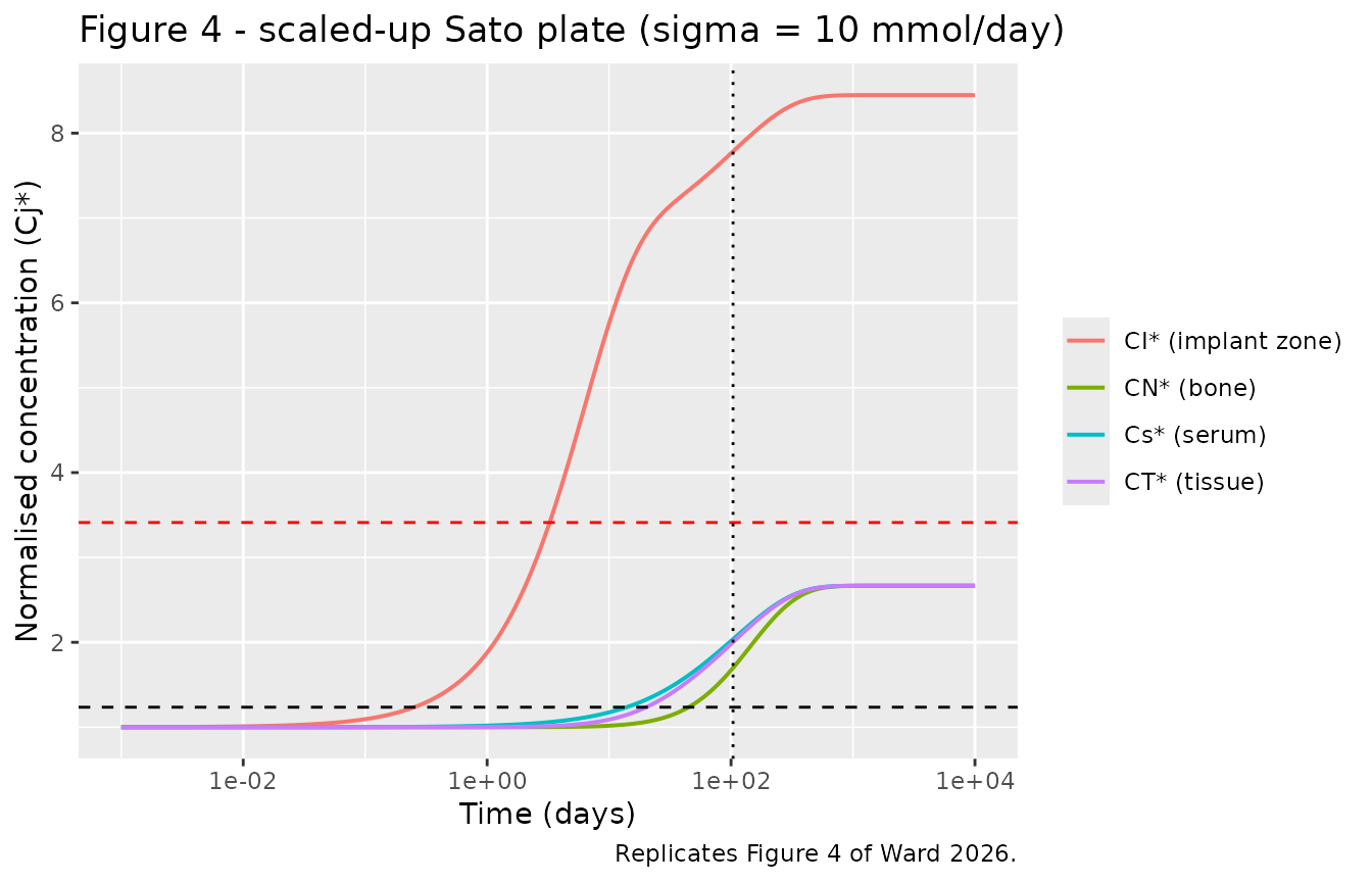
The implant zone settles at CI* = 8.45, the roughly
eight-fold local increase the paper reports, and serum rises to
Cs* = 2.67 – well past the hypermagnesemia threshold but
below the “dangerous” level of 3.41.
Figure 7 – reduced kidney function and dietary control
For a patient with severely compromised renal function the paper sets
gamma = gamma_0 / 3 with a matched reduction of
phi_D so that pre-implant homeostasis is unchanged, then
modulates external Mg intake by the factor rho (eq 10). The
steady states of eqs 2-4 with eq 10 are given by eq 11, and eq 12 gives
the intake reduction that restores homeostasis exactly:
rho = 1 - sigma / phi_D
gam_ckd  <- gam0 / 3   # severely compromised kidney function
phiD_ckd <- phiD / 3   # matched, so Cse = phiD/gamma is unchanged
n_ckd    <- 20
sig_ckd  <- n_ckd * 0.05
rho_star <- 1 - sig_ckd / phiD_ckd     # eq 12
rho_star
#> [1] 0.5

f7 <- lapply(c(0, 0.25, 0.5, 0.75, 1), function(r) {
  solve_scenario(times = t_log, n_implant = n_ckd, f_diet = r,
                 rate_diet = phiD_ckd, cl_renal = gam_ckd) |>
    transmute(time, rho = factor(r), Cs_norm, CI_norm)
}) |> bind_rows() |> filter(time > 0)

ggplot(filter(f7, time >= 1e-2), aes(time, Cs_norm, colour = rho)) +
  geom_line(linewidth = 0.6) +
  geom_hline(yintercept = c(1, Chyp_norm), linetype = c("solid", "dashed"),
             colour = c("grey60", "black")) +
  geom_vline(xintercept = TMg_formula, linetype = "dotted") +
  scale_x_log10(limits = c(1e-2, 1e4)) +
  labs(x = "Time (days)", y = "Cs* (normalised serum)", colour = "rho",
       title = "Figure 7A - dietary control, n = 20, gamma = gamma_0/3",
       caption = "Replicates Figure 7A of Ward 2026. Grey line: homeostasis.")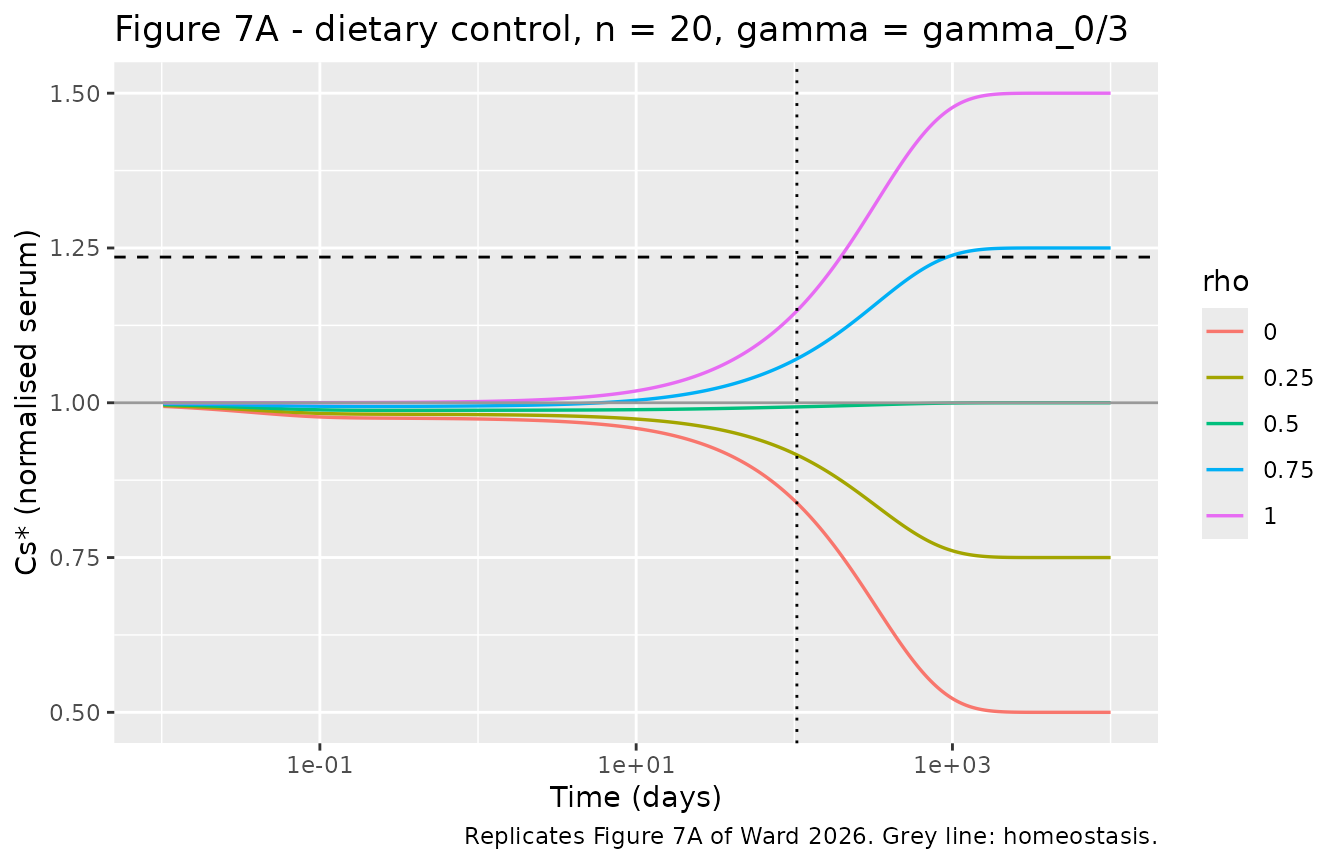
The eq 11 steady states, and the eq 12 exact-homeostasis result, both reproduce:
eq11 <- function(rho, n, phiD_l, gam_l) {
  sig <- n * 0.05
  xi  <- n * xi0
  c(Cs = rho + sig / phiD_l,
    CI = rho + sig / phiD_l + sig * gam_l / (xi * k1 * phiD_l))
}

eq11_chk <- lapply(c(0, 0.25, 0.5, 0.75, 1), function(r) {
  s <- solve_scenario(times = t_log, n_implant = n_ckd, f_diet = r,
                      rate_diet = phiD_ckd, cl_renal = gam_ckd)
  p <- eq11(r, n_ckd, phiD_ckd, gam_ckd)
  tibble(rho = r,
         Cs_sim = tail(s$Cs_norm, 1), Cs_eq11 = unname(p["Cs"]),
         CI_sim = tail(s$CI_norm, 1), CI_eq11 = unname(p["CI"]))
}) |> bind_rows()

eq11_chk |>
  mutate(across(-rho, ~ signif(.x, 6))) |>
  dplyr::rename("rho" = rho, "Cs* (sim)" = Cs_sim, "Cs* (eq 11)" = Cs_eq11,
                "CI* (sim)" = CI_sim, "CI* (eq 11)" = CI_eq11) |>
knitr::kable(caption = "Dietary control: simulated steady states vs eq 11.")| rho | Cs* (sim) | Cs* (eq 11) | CI* (sim) | CI* (eq 11) |
|---|---|---|---|---|
| 0.00 | 0.50 | 0.50 | 7.08213 | 7.08213 |
| 0.25 | 0.75 | 0.75 | 7.33213 | 7.33213 |
| 0.50 | 1.00 | 1.00 | 7.58213 | 7.58213 |
| 0.75 | 1.25 | 1.25 | 7.83213 | 7.83213 |
| 1.00 | 1.50 | 1.50 | 8.08213 | 8.08213 |
# eq 12: halving intake restores homeostasis exactly for this scenario.
cs_at_rho_star <- tail(
  solve_scenario(times = t_log, n_implant = n_ckd, f_diet = rho_star,
                 rate_diet = phiD_ckd, cl_renal = gam_ckd)$Cs_norm, 1)
c(rho_star = rho_star, Cs_star = cs_at_rho_star)
#> rho_star  Cs_star
#>      0.5      1.0

stopifnot(
  max(abs(eq11_chk$Cs_sim - eq11_chk$Cs_eq11)) < 1e-6,
  max(abs(eq11_chk$CI_sim - eq11_chk$CI_eq11)) < 1e-4,
  abs(rho_star - 0.5) < 1e-12,
  abs(cs_at_rho_star - 1) < 1e-5
)
The early-phase dip
Cutting dietary intake at t = 0 while the implant
contribution is still building produces a fast drop in serum Mg over the
first day or so, before the slow implant-driven rise takes over. Section
2.3.1 quantifies it with a minimum-concentration formula and states that
“the maximum drop is predicted to be about 8% of homeostatic levels when
Mg intake is zero”, using the healthy Table 1 parameters.
The printed formula is mangled in the typeset PDF (see Errata below); the reading consistent with the paper’s own quoted 8% is
Cs*_min ~= 1 + (rho - 1) * Gamma, Gamma = gamma / k_1which is the dimensionless group Gamma the paper defines
in Section 2.2.3.
Gamma0 <- gam0 / k1
Gamma0                       # paper prints Gamma_0 ~= 0.0787
#> [1] 0.07898551

# Healthy parameters, intake cut to zero: measure the fast-phase minimum before
# the slow systemic rise sets in (the paper's "around 1-10 days" window).
dip <- solve_scenario(times = seq(0, 1, length.out = 2001),
                      n_implant = 20, f_diet = 0)
dip_pct     <- 100 * (1 - tail(dip$Cs_norm, 1))
formula_pct <- 100 * Gamma0

c(simulated_drop_pct = dip_pct, formula_drop_pct = formula_pct)  # paper: "about 8%"
#> simulated_drop_pct   formula_drop_pct
#>           7.800151           7.898551

stopifnot(abs(dip_pct - formula_pct) < 0.5, abs(formula_pct - 8) < 1)
The simulated fast-phase drop is 7.8% against the formula’s 7.9%, matching the paper’s “about 8%” and confirming the intended reading of the printed equation.
Assumptions, deviations and errata
No IIV and no residual error. The publication is a deterministic mechanistic simulation of an “average” individual and reports neither a variance model nor a residual-error model. None is invented; the model file carries typical values only, all wrapped in
fixed().Initial conditions are computed, not transcribed.
serum(0)etc. are set from eq 5 (rate_diet / cl_renaland the exchange ratios) rather than from Table 1’s printed homeostatic concentrations. Table 1’sgamma = 10.9is the rounded form ofphi_D / Cse = 6 / 0.5525 = 10.86, sophi_D / gamma = 0.5505differs from the printedCse = 0.553by 0.4%. Seeding from the printed value would leave the model 0.4% off its own steady state and destroy the exact-homeostasis check above. The same rounding chain explainsCNe42.97 vs the printed 43.1,CTe2.189 vs 2.20, andGamma_00.0790 vs the printed 0.0787.V_Tin eq 3 isV_Ttot, not(1 - xi) V_Ttot. The(1 - xi)factor appears only on the right-hand side flux. This is settled by Supporting Information B (S15), “V_I is chosen so that V_I/V_T = 0.0001 giving V_I = 5.27 ml”, and independently by Table 2’sT_1 = V_T (1 + xi_3) / k_-1, which evaluates to 6.07 days only with the full 52.7 L.Erratum – the Supporting Information contradicts Table 1 on one ratio. Supporting Information B (p. S12) states
mu_-1 / mu_1 ~= Cse / CNe ~= 0.0385. Table 1’s own values give0.0775 / 6.05 = 0.01281, andCse / CNe = 0.553 / 43.1 = 0.01282. The prose figure is a factor of three too large (0.0385 = 3 x 0.0128). Table 1 is self-consistent and is used here: back-solving the prose ratio would forcemu_-1 = 0.233andCNe = 14.3, contradicting Table 1’s printedCNe = 43.1and breaking the eq 8 steady states that the simulations above reproduce exactly.Erratum – Section 2.3.1’s minimum-concentration formula is mangled. It is typeset as
C*_smin ~= 1 + (rho - 1)/gamma k_1, which is not reconstructible as printed. The reading1 + (rho - 1) * gamma / k_1gives 7.9% forrho = 0, matching both the paper’s own quoted “about 8%” and the simulated fast-phase drop of 7.8%; no other grouping of the same symbols does (1/(gamma k_1)gives 0.07%). That reading is used in the check above and is the dimensionlessGamma = gamma / k_1defined in Section 2.2.3.Erratum – Figure 6 axis label. The x-axis of Figure 6 is labelled
sigma (mmol/L);sigmais a release rate in mmol/day everywhere else in the paper, including Table 1 and the Figure 6 caption’s own text.V_Iis a modelling choice, not a measurement. The peri-implant zone has no anatomic boundary. The authors pickV_I / V_Ttot = 1e-4(5.27 mL, about 20 times the volume of the screw itself) and note thatC_Iscales as1 / V_Iwhile serum, bone and tissue predictions are insensitive to it. The paper explicitly says its implant-region predictions “underestimate the recorded Mg excretion rate and the rate of Mg increase in localized tissue concentration; though quantitative agreement for the latter can be tuned by decreasing the volumeV_I.”Scenario levers are
ini()parameters.n_implant(eq 9) andf_diet(rho, eq 10) are fixed at 1 in the packaged model, i.e. one screw and normal dietary intake. They are varied above by re-pinning them, which is how every published figure is reproduced. They are not estimated quantities.No non-compartmental analysis. There is no dose and no absorption-distribution-elimination profile, so PKNCA is not an applicable validation and is deliberately omitted in favour of the steady-state, closed-form, time-constant and perturbation checks above.