Buprenorphine depot opioid blockade (Walsh 2024)
Source:vignettes/articles/Walsh_2024_buprenorphine_opioidBlockade.Rmd
Walsh_2024_buprenorphine_opioidBlockade.RmdModel and source
Walsh et al. (2024) report three independent
exposure-response analyses of opioid blockade by CAM2038, a subcutaneous
long-acting buprenorphine (BPN) depot, in non-treatment-seeking adults
with moderate to severe opioid use disorder. Each endpoint was fitted as
its own NONMEM analysis with a different structure, a different
transformation, and (for drug liking) a different NONMEM version, so the
paper contributes three model files to nlmixr2lib:
| Model | Endpoint | Structure |
|---|---|---|
Walsh_2024_buprenorphine_drugLiking |
Period-corrected drug liking Emax bipolar VAS score | Direct Imax, logit-transformed onto -1 to 52 |
Walsh_2024_buprenorphine_desireToUse |
Desire to use unipolar VAS score (0-100 mm) | Imax with exponential onset delay, logit-transformed onto -1 to 101 |
Walsh_2024_buprenorphine_cows |
Clinical Opiate Withdrawal Scale total score (0-44) | Bounded-integer Imax between two probit-scale asymptotes |
Supplementary Appendix:
41386_2023_1793_MOESM1_ESM.pdf(Tables S1-S4 and all three structural equations)Underlying phase 2 study (NCT02611752): https://doi.org/10.1001/jamapsychiatry.2017.1874
Citation: Walsh SL, Comer SD, Aguiar Zdovc J, Sarr C, Bjornsson M, Strandgarden K, Hjelmstrom P, Tiberg F. Pharmacokinetic-pharmacodynamic analysis of drug liking blockade by buprenorphine subcutaneous depot (CAM2038) in participants with opioid use disorder. Neuropsychopharmacology. 2024;49(6):1050-1057. doi:10.1038/s41386-023-01793-z. Parameter estimates from Table 1; structural equation and the logit residual-error transformation from the Supplementary Appendix (41386_2023_1793_MOESM1_ESM.pdf). Underlying phase 2 study NCT02611752, reported in Walsh SL, Comer SD, Lofwall MR, et al. JAMA Psychiatry. 2017;74(9):894-902. doi:10.1001/jamapsychiatry.2017.1874. Sister endpoint models from the same paper: modellib(‘Walsh_2024_buprenorphine_desireToUse’).
These are PD-only models
All three models are static algebraic exposure-response
relationships. They contain no ODE, no compartments and no
dosing events. The driver is the covariate column
CP_BPN_NGML, the time-matched buprenorphine plasma
concentration in ng/mL, which must be supplied per observation
record.
The CAM2038 population PK model is not reported in Walsh
2024 and no buprenorphine popPK model is packaged in
nlmixr2lib, so a user who wants to drive these models from
a dose regimen must supply concentrations from an external PK source.
Because there is no PK model and no dosing, a PKNCA non-compartmental
analysis is not meaningful here; this vignette validates the models
against the paper’s own reported exposure-response quantities
instead.
Population
pop <- drugLiking$meta$population
tibble::tibble(
  Field = c(
    "Species", "Participants", "Studies", "Age", "Body weight",
    "Female", "Race", "Disease state", "Regions"
  ),
  Value = c(
    pop$species,
    as.character(pop$n_subjects),
    as.character(pop$n_studies),
    pop$age_range,
    pop$weight_range,
    paste0(pop$sex_female_pct, "%"),
    paste(names(pop$race_ethnicity), pop$race_ethnicity,
          sep = ": ", collapse = "%, "),
    pop$disease_state,
    pop$regions
  )
) |>
knitr::kable()| Field | Value |
|---|---|
| Species | human |
| Participants | 47 |
| Studies | 1 |
| Age | 18-54 years (median 36.0; mean 35.8, SD 9.1) |
| Body weight | 53.0-110.0 kg (median 73.4; mean 75.9, SD 14.0) |
| Female | 25.5% |
| Race | Black: 51%, White: 47%, Other: 2 |
| Disease state | Non-treatment-seeking adults with moderate to severe opioid use disorder (DSM-5), physically dependent on opioids. |
| Regions | USA (multisite: University of Kentucky; Columbia University / New York State Psychiatric Institute) |
Forty-seven participants were randomised 1:1, stratified by sex, to CAM2038 24 mg (n = 22) or 32 mg (n = 25) once weekly on days 0 and 7. Intramuscular hydromorphone challenges of 0, 6 or 18 mg were given once daily over each of the day -3 to -1, 1-3, 4-6, 8-10 and 11-13 periods. BPN plasma samples were drawn approximately 60 min before each hydromorphone administration, giving one time-matched concentration per challenge day.
The three endpoints used different subsets of those challenge days (Supplementary Table S2):
tibble::tibble(
  Endpoint = c("Drug liking Emax VAS", "Desire to use VAS", "COWS"),
  `24 mg` = c(109L, 328L, 284L),
  `32 mg` = c(122L, 364L, 314L),
  Total = c(231L, 692L, 598L),
  `Challenge doses used` = c(
    "18 mg only (0 and 6 mg gave no or lower responses)",
    "0, 6 and 18 mg (pre-challenge score analysed)",
    "0, 6 and 18 mg (assessed before the challenge)"
  )
) |>
knitr::kable(caption = "Analysis datasets (Walsh 2024 Table S2).")| Endpoint | 24 mg | 32 mg | Total | Challenge doses used |
|---|---|---|---|---|
| Drug liking Emax VAS | 109 | 122 | 231 | 18 mg only (0 and 6 mg gave no or lower responses) |
| Desire to use VAS | 328 | 364 | 692 | 0, 6 and 18 mg (pre-challenge score analysed) |
| COWS | 284 | 314 | 598 | 0, 6 and 18 mg (assessed before the challenge) |
Source trace
Every ini() value below was read from the paper or its
Supplementary Appendix. The observed BPN plasma concentration range
across the study was 0.636-12.3 ng/mL.
tibble::tribble(
  ~Parameter, ~Value, ~Source,
  "lbase", "log(45.3) VAS units", "Table 1, drug liking block (RSE 2.40%)",
  "lic50", "log(0.075) ng/mL", "Table 1, drug liking block (RSE 30.4%)",
  "imax", "1 (FIX)", "Table 1, drug liking block: Imax 1.00 (FIX)",
  "hill", "1 (FIX)", "Results, Model development: 'Imax and gamma were fixed to 1'",
  "etalbase", "0.106^2", "Table 1: IIV Baseline SD 0.106 (RSE 19.8%, shrinkage 11.6%)",
  "etalic50", "1.90^2", "Table 1: IIV IC50 SD 1.90 (RSE 10.3%, shrinkage 13.3%)",
  "addSd", "0.744", "Table 1: Additive RUV (logit scale) 0.744 (RSE 8.62%)",
  "Structure", "VAS = BASE * (1 - Imax * Cp^g / (IC50^g + Cp^g))", "Methods, Model development",
  "Error", "logitNorm(addSd, -1, 52)", "Supplementary Methods, RUV equations (TI = (yhat + 1) / 53)"
) |>
knitr::kable(caption = "Source trace: Walsh_2024_buprenorphine_drugLiking.")| Parameter | Value | Source |
|---|---|---|
| lbase | log(45.3) VAS units | Table 1, drug liking block (RSE 2.40%) |
| lic50 | log(0.075) ng/mL | Table 1, drug liking block (RSE 30.4%) |
| imax | 1 (FIX) | Table 1, drug liking block: Imax 1.00 (FIX) |
| hill | 1 (FIX) | Results, Model development: ‘Imax and gamma were fixed to 1’ |
| etalbase | 0.106^2 | Table 1: IIV Baseline SD 0.106 (RSE 19.8%, shrinkage 11.6%) |
| etalic50 | 1.90^2 | Table 1: IIV IC50 SD 1.90 (RSE 10.3%, shrinkage 13.3%) |
| addSd | 0.744 | Table 1: Additive RUV (logit scale) 0.744 (RSE 8.62%) |
| Structure | VAS = BASE * (1 - Imax * Cp^g / (IC50^g + Cp^g)) | Methods, Model development |
| Error | logitNorm(addSd, -1, 52) | Supplementary Methods, RUV equations (TI = (yhat + 1) / 53) |
tibble::tribble(
  ~Parameter, ~Value, ~Source,
  "logitbase", "logit(92.5, -1, 101)", "Table S3: Baseline 92.5 VAS units (RSE 0.296%)",
  "lambda_base", "-12.9", "Table S3: Baseline Box-Cox shape parameter (RSE 4.91%)",
  "lic50", "log(0.0129) ng/mL", "Table S3: IC50 0.0129 ng/mL (RSE 12.3%)",
  "imax", "1 (FIX)", "Table S3: Imax 1.00 (FIXED)",
  "hill", "1 (FIX)", "Supplementary Methods: 'The sigmoidicity parameter, gamma, was fixed to 1'",
  "lthalf_onset", "log(0.330) day", "Table S3: Onset half-life 0.330 day (RSE 18.7%)",
  "etalogitbase", "0.167^2", "Table S3: IIV Baseline 0.167 (RSE 14.1%, shrinkage 5.76%)",
  "etalic50", "9.29^2", "Table S3: IIV IC50 9.29 (RSE 21.7%, shrinkage 42.2%)",
  "etalthalf_onset", "1.91^2", "Table S3: IIV onset half-life 1.91 (RSE 17.6%, shrinkage 33.9%)",
  "addSd", "0.783", "Table S3: RUV 0.783 (RSE 8.45%, shrinkage 5.68%)",
  "Structure", "IPRED = BASE * (1 - Imax(t) * Cp^g / (IC50^g + Cp^g))", "Supplementary Methods, Desire to use VAS score",
  "Onset delay", "Imax(t) = TVImax * (1 - exp(-kt * time))", "Supplementary Methods, Desire to use VAS score",
  "Error", "logitNorm(addSd, -1, 101)", "Supplementary Methods (TI = (yhat + 1) / 102)"
) |>
knitr::kable(caption = "Source trace: Walsh_2024_buprenorphine_desireToUse.")| Parameter | Value | Source |
|---|---|---|
| logitbase | logit(92.5, -1, 101) | Table S3: Baseline 92.5 VAS units (RSE 0.296%) |
| lambda_base | -12.9 | Table S3: Baseline Box-Cox shape parameter (RSE 4.91%) |
| lic50 | log(0.0129) ng/mL | Table S3: IC50 0.0129 ng/mL (RSE 12.3%) |
| imax | 1 (FIX) | Table S3: Imax 1.00 (FIXED) |
| hill | 1 (FIX) | Supplementary Methods: ‘The sigmoidicity parameter, gamma, was fixed to 1’ |
| lthalf_onset | log(0.330) day | Table S3: Onset half-life 0.330 day (RSE 18.7%) |
| etalogitbase | 0.167^2 | Table S3: IIV Baseline 0.167 (RSE 14.1%, shrinkage 5.76%) |
| etalic50 | 9.29^2 | Table S3: IIV IC50 9.29 (RSE 21.7%, shrinkage 42.2%) |
| etalthalf_onset | 1.91^2 | Table S3: IIV onset half-life 1.91 (RSE 17.6%, shrinkage 33.9%) |
| addSd | 0.783 | Table S3: RUV 0.783 (RSE 8.45%, shrinkage 5.68%) |
| Structure | IPRED = BASE * (1 - Imax(t) * Cp^g / (IC50^g + Cp^g)) | Supplementary Methods, Desire to use VAS score |
| Onset delay | Imax(t) = TVImax * (1 - exp(-kt * time)) | Supplementary Methods, Desire to use VAS score |
| Error | logitNorm(addSd, -1, 101) | Supplementary Methods (TI = (yhat + 1) / 102) |
tibble::tribble(
  ~Parameter, ~Value, ~Source,
  "probitbase", "-0.887", "Table S4: BASEb.int (RSE 8.67%)",
  "probitbase_low", "-2.11", "Table S4: LBASEb.int (RSE 4.58%)",
  "lic90", "log(0.109) ng/mL", "Table S4: IC90 0.109 ng/mL (RSE 43.1%)",
  "hill", "1 (FIX)", "Supplementary Methods: 'the sigmoidicity, gamma, was fixed to 1'",
  "addSd", "0.265", "Table S4: SDb.int scaling parameter (RSE 5.66%)",
  "IIV block", "0.454^2, corr 0.0203, 0.0948^2", "Table S4: IIV BASEb.int 0.454, IIV LBASEb.int 0.0948, correlation 0.0203 (RSE 478%)",
  "Structure", "IPRED = BASEb.int - (BASEb.int - LBASEb.int) * Cp^g / (IC50^g + Cp^g)", "Supplementary Methods, COWS score (third and final variant)",
  "IC50 recovery", "IC50 = IC90 / 9^(1/g)", "Supplementary Methods: 'the IC90 was estimated instead of the IC50'",
  "Error", "probitNorm(addSd, 0, 45)", "Supplementary Methods: bounded integer model of Ueckert & Karlsson (2021)"
) |>
knitr::kable(caption = "Source trace: Walsh_2024_buprenorphine_cows.")| Parameter | Value | Source |
|---|---|---|
| probitbase | -0.887 | Table S4: BASEb.int (RSE 8.67%) |
| probitbase_low | -2.11 | Table S4: LBASEb.int (RSE 4.58%) |
| lic90 | log(0.109) ng/mL | Table S4: IC90 0.109 ng/mL (RSE 43.1%) |
| hill | 1 (FIX) | Supplementary Methods: ‘the sigmoidicity, gamma, was fixed to 1’ |
| addSd | 0.265 | Table S4: SDb.int scaling parameter (RSE 5.66%) |
| IIV block | 0.454^2, corr 0.0203, 0.0948^2 | Table S4: IIV BASEb.int 0.454, IIV LBASEb.int 0.0948, correlation 0.0203 (RSE 478%) |
| Structure | IPRED = BASEb.int - (BASEb.int - LBASEb.int) * Cp^g / (IC50^g + Cp^g) | Supplementary Methods, COWS score (third and final variant) |
| IC50 recovery | IC50 = IC90 / 9^(1/g) | Supplementary Methods: ‘the IC90 was estimated instead of the IC50’ |
| Error | probitNorm(addSd, 0, 45) | Supplementary Methods: bounded integer model of Ueckert & Karlsson (2021) |
Validation
The paper reports several quantities that are exact algebraic consequences of the fitted parameters. Each is used below as a gate on the packaged models.
Gate 1: baseline recovery at zero buprenorphine
At CP_BPN_NGML = 0 every model must return its published
baseline. For COWS the published baseline is on the probit scale, so the
observable score is 45 * pnorm(-0.887).
zero_ev <- function(cp, times = 0) {
  tidyr::expand_grid(id = seq_along(cp), time = times) |>
    dplyr::mutate(CP_BPN_NGML = cp[id], evid = 0L, amt = 0)
}

dl0 <- rxode2::rxSolve(drugLiking, zero_ev(0), omega = NA,
                       returnType = "data.frame")
# Imax has fully onset by day 14, so the baseline check is not confounded by
# the onset-delay term.
dtu0 <- rxode2::rxSolve(desireToUse, zero_ev(0, times = c(0, 14)), omega = NA,
                        returnType = "data.frame")
cows0 <- rxode2::rxSolve(cows, zero_ev(0), omega = NA, returnType = "data.frame")

baseline <- tibble::tibble(
  Endpoint = c("Drug liking Emax VAS", "Desire to use VAS", "COWS total score"),
  Simulated = c(
    dl0$druglikingvascfb[1],
    dtu0$desiretousevas[nrow(dtu0)],
    cows0$cows[1]
  ),
  Published = c(45.3, 92.5, 45 * pnorm(-0.887)),
  Source = c("Table 1", "Table S3", "Table S4 (BASEb.int back-transformed)")
) |>
  dplyr::mutate(
    Simulated = round(Simulated, 3),
    Published = round(Published, 3),
    `Difference (%)` = round(100 * (Simulated - Published) / Published, 3)
  )

knitr::kable(baseline, caption = "Gate 1: baseline recovery at Cp = 0.")| Endpoint | Simulated | Published | Source | Difference (%) |
|---|---|---|---|---|
| Drug liking Emax VAS | 45.300 | 45.300 | Table 1 | 0 |
| Desire to use VAS | 92.500 | 92.500 | Table S3 | 0 |
| COWS total score | 8.439 | 8.439 | Table S4 (BASEb.int back-transformed) | 0 |
The COWS pre-treatment score of 8.4 sits inside the 5-12 band the paper describes as mild withdrawal symptoms, which is the clinically expected state for this opioid-dependent cohort before treatment.
Gate 2: IC50 and IC90 identities
For a sigmoid Imax model, IC90 = IC50 * 9^(1/gamma).
With gamma fixed to 1 this reduces to
IC90 = 9 * IC50. The paper reports the IC90 for all three
endpoints independently of the IC50 it tabulates, so reproducing them is
a direct check that gamma = 1 and Imax = 1 are
encoded as the authors intended. Equivalently, the simulated response at
the IC50 must be exactly 50% of baseline and at the IC90 exactly 10% of
baseline.
ic50_dl <- 0.075
ic50_dtu <- 0.0129
ic90_cows <- 0.109
ic50_cows <- ic90_cows / 9

dl_sweep <- rxode2::rxSolve(
  drugLiking, zero_ev(c(0, ic50_dl, 9 * ic50_dl)), omega = NA,
  returnType = "data.frame"
)
#> Warning: multi-subject simulation without without 'omega'
dtu_sweep <- rxode2::rxSolve(
  desireToUse, zero_ev(c(0, ic50_dtu, 9 * ic50_dtu), times = c(0, 14)),
  omega = NA, returnType = "data.frame"
) |>
  dplyr::filter(time == 14)
#> Warning: multi-subject simulation without without 'omega'

ic <- tibble::tibble(
  Endpoint = c("Drug liking Emax VAS", "Desire to use VAS", "COWS total score"),
  `IC50 (ng/mL)` = c(ic50_dl, ic50_dtu, ic50_cows),
  `IC90 simulated (ng/mL)` = c(9 * ic50_dl, 9 * ic50_dtu, ic90_cows),
  `IC90 published (ng/mL)` = c(0.675, 0.116, 0.109),
  `IC90 / IC50` = c(9, 9, ic90_cows / ic50_cows)
) |>
  dplyr::mutate(dplyr::across(dplyr::where(is.numeric), \(x) round(x, 4)))

knitr::kable(
  ic,
  caption = paste(
    "Gate 2: IC90 = 9 * IC50 identities. The COWS row is inverted because",
    "the authors estimated IC90 and Table S4 reports the derived IC50."
  )
)| Endpoint | IC50 (ng/mL) | IC90 simulated (ng/mL) | IC90 published (ng/mL) | IC90 / IC50 |
|---|---|---|---|---|
| Drug liking Emax VAS | 0.0750 | 0.6750 | 0.675 | 9 |
| Desire to use VAS | 0.0129 | 0.1161 | 0.116 | 9 |
| COWS total score | 0.0121 | 0.1090 | 0.109 | 9 |
# Drug liking and desire to use: 9 * IC50 must reproduce the published IC90.
stopifnot(abs(9 * ic50_dl - 0.675) < 1e-9)
stopifnot(abs(9 * ic50_dtu - 0.116) < 5e-4)
# COWS: IC90 / 9 must reproduce the IC50 Table S4 reports as derived.
stopifnot(abs(ic50_cows - 0.012) < 5e-4)
For drug liking and desire to use, Imax is fixed to 1,
so the effect runs all the way to zero and the response at the IC50 and
IC90 must be exactly one half and one tenth of baseline. COWS is
different: its effect runs between two probit-scale asymptotes, so the
quantity that must hit one half and nine tenths is the fraction of the
maximal decrease (BASEb.int - LBASEb.int)
that has been achieved.
cows_sweep <- rxode2::rxSolve(
  cows, zero_ev(c(0, ic50_cows, ic90_cows)), omega = NA,
  returnType = "data.frame"
)
#> Warning: multi-subject simulation without without 'omega'

fractions <- tibble::tibble(
  Endpoint = c("Drug liking Emax VAS", "Desire to use VAS", "COWS total score"),
  Quantity = c(
    "Response / baseline", "Response / baseline",
    "Achieved decrease / maximal decrease"
  ),
  `At IC50` = c(
    dl_sweep$druglikingvascfb[2] / dl_sweep$druglikingvascfb[1],
    dtu_sweep$desiretousevas[2] / dtu_sweep$desiretousevas[1],
    (cows_sweep$pbase[2] - cows_sweep$latentcows[2]) /
      (cows_sweep$pbase[2] - cows_sweep$pbase_low[2])
  ),
  `At IC90` = c(
    dl_sweep$druglikingvascfb[3] / dl_sweep$druglikingvascfb[1],
    dtu_sweep$desiretousevas[3] / dtu_sweep$desiretousevas[1],
    (cows_sweep$pbase[3] - cows_sweep$latentcows[3]) /
      (cows_sweep$pbase[3] - cows_sweep$pbase_low[3])
  ),
  `Expected at IC50` = c(0.5, 0.5, 0.5),
  `Expected at IC90` = c(0.1, 0.1, 0.9)
) |>
  dplyr::mutate(dplyr::across(dplyr::where(is.numeric), \(x) round(x, 4)))

knitr::kable(
  fractions,
  caption = "Gate 2b: exact half-maximal and 90%-maximal behaviour."
)| Endpoint | Quantity | At IC50 | At IC90 | Expected at IC50 | Expected at IC90 |
|---|---|---|---|---|---|
| Drug liking Emax VAS | Response / baseline | 0.5 | 0.1 | 0.5 | 0.1 |
| Desire to use VAS | Response / baseline | 0.5 | 0.1 | 0.5 | 0.1 |
| COWS total score | Achieved decrease / maximal decrease | 0.5 | 0.9 | 0.5 | 0.9 |
Gate 3: desire-to-use onset half-life
The desire to use model is the only one of the three that is not
direct: a delay in the onset of effect is carried by
Imax(t) = TVImax * (1 - exp(-kt * t)) with
kt = log(2) / 0.330 per day. At t = 0 there is
no effect, and at t = 0.330 day exactly half of the maximum
inhibition is in place.
onset <- rxode2::rxSolve(
  desireToUse,
  data.frame(
    id = 1L, time = c(0, 0.330, 0.660, 1, 2, 7),
    CP_BPN_NGML = 0, evid = 0L, amt = 0
  ),
  omega = NA, returnType = "data.frame"
) |>
  dplyr::transmute(
    `Time (day)` = time,
    `Imax(t)` = round(imax_t, 4),
    `Expected` = round(1 - exp(-log(2) / 0.330 * time), 4)
  )

knitr::kable(onset, caption = "Gate 3: onset of the maximum inhibitory effect.")| Time (day) | Imax(t) | Expected |
|---|---|---|
| 0.00 | 0.0000 | 0.0000 |
| 0.33 | 0.5000 | 0.5000 |
| 0.66 | 0.7500 | 0.7500 |
| 1.00 | 0.8776 | 0.8776 |
| 2.00 | 0.9850 | 0.9850 |
| 7.00 | 1.0000 | 1.0000 |
Replicating Figure 4: drug liking exposure-response
Figure 4 of Walsh 2024 plots the period-corrected drug liking Emax
VAS score against BPN plasma concentration, with the typical prediction
and a 2.5th-97.5th percentile band simulated with parameter
uncertainty. The paper draws 10,000 parameter sets from the
estimated covariance matrix; that matrix is not published, so the band
below is reproduced by drawing 200 sets from independent log-normal
distributions using the reported relative standard errors
(Baseline 2.40%, IC50 30.4%). Ignoring the
off-diagonal terms is an approximation and is recorded under Assumptions
below.
n_draw <- 200L
cp_grid <- c(seq(0.01, 0.5, by = 0.01), seq(0.55, 3, by = 0.05))

ini_dl <- drugLiking$iniDf
est <- function(nm) ini_dl$est[ini_dl$name == nm]
sd_log <- function(rse) sqrt(log(1 + rse^2))

# Re-seed immediately before the draws. The set.seed() at the top of this file
# is NOT sufficient: rxode2::rxSolve() consumes R's RNG stream even when called
# with omega = NA, and seven solves run above this point. How far the stream is
# advanced depends on the rxode2 version, the number of observation rows and
# the threading, so the same top-of-file seed lands on a different position on
# a different machine. That is exactly how this chunk passed locally and failed
# in CI: a different draw put every upper 97.5% limit above the 11-point
# threshold, so the crossing below came back NA. Seeding here makes the band
# depend only on this chunk.
set.seed(20240501)

base_draw <- exp(est("lbase") + rnorm(n_draw, 0, sd_log(0.0240)))
ic50_draw <- exp(est("lic50") + rnorm(n_draw, 0, sd_log(0.304)))

# The uncertainty band is evaluated in closed form rather than by solving one
# id per draw.
#
# Why: rxode2::rxSolve() with a multi-row `params` data.frame does not return
# the same values for byte-identical inputs. Holding the draws fixed (verified
# by hashing them), five successive solves in one session produced five
# different result hashes and crossings of 0.45, 0.60, 0.45, 2.30 and 0.46 --
# and sometimes no crossing at all. That is what made this chunk pass locally
# and fail in CI; it is not a seeding problem, and re-seeding does not fix it.
#
# Confirmed present on rxode2 5.1.7 (origin/main @ 7d74e29e4), not only on the
# 5.1.3 release, so this workaround is still required. It appears at >= 8
# subjects and is independent of core count -- `cores = 1` fails too. The
# maintainers keep a reprex that records when this can be reverted.
#
# Doing the arithmetic here is safe because the drug liking model is algebraic
# in Cp with Imax and gamma both fixed to 1, and the closed form was checked to
# reproduce a (correct) solve exactly -- max absolute difference 0. The
# stopifnot below re-checks that identity against the typical-value solve on
# every render, so if the model equation ever changes this fails loudly instead
# of quietly plotting stale arithmetic.
vas_curve <- function(cp, base, ic50) base * (1 - cp / (ic50 + cp))

unc <- tibble::tibble(
  CP_BPN_NGML = cp_grid,
  lo = vapply(cp_grid, function(cp)
    quantile(vas_curve(cp, base_draw, ic50_draw), 0.025, names = FALSE), numeric(1)),
  hi = vapply(cp_grid, function(cp)
    quantile(vas_curve(cp, base_draw, ic50_draw), 0.975, names = FALSE), numeric(1))
)

typ <- rxode2::rxSolve(
  drugLiking, zero_ev(cp_grid), omega = NA, returnType = "data.frame"
) |>
  dplyr::transmute(CP_BPN_NGML, typical = druglikingvascfb)
#> Warning: multi-subject simulation without without 'omega'

fig4 <- dplyr::left_join(typ, unc, by = "CP_BPN_NGML")

# The typical curve still comes from the model. Check that the closed form used
# for the band above reproduces it, so the band cannot silently drift from the
# model equation. This is a single-subject solve, which is not affected by the
# multi-row `params` problem described above.
stopifnot(isTRUE(all.equal(
  fig4$typical,
  vas_curve(fig4$CP_BPN_NGML, exp(est("lbase")), exp(est("lic50"))),
  tolerance = 1e-8
)))

ggplot2::ggplot(fig4, ggplot2::aes(x = CP_BPN_NGML)) +
  ggplot2::geom_ribbon(ggplot2::aes(ymin = lo, ymax = hi),
                       fill = "steelblue", alpha = 0.25) +
  ggplot2::geom_line(ggplot2::aes(y = typical), colour = "steelblue",
                     linewidth = 1) +
  ggplot2::geom_hline(yintercept = 11, linetype = "dashed") +
  ggplot2::scale_x_log10() +
  ggplot2::labs(
    x = "BPN plasma concentration (ng/mL, log scale)",
    y = "Period-corrected drug liking Emax VAS score",
    caption = "Dashed line: 11-point complete blockade threshold."
  ) +
  ggplot2::theme_bw()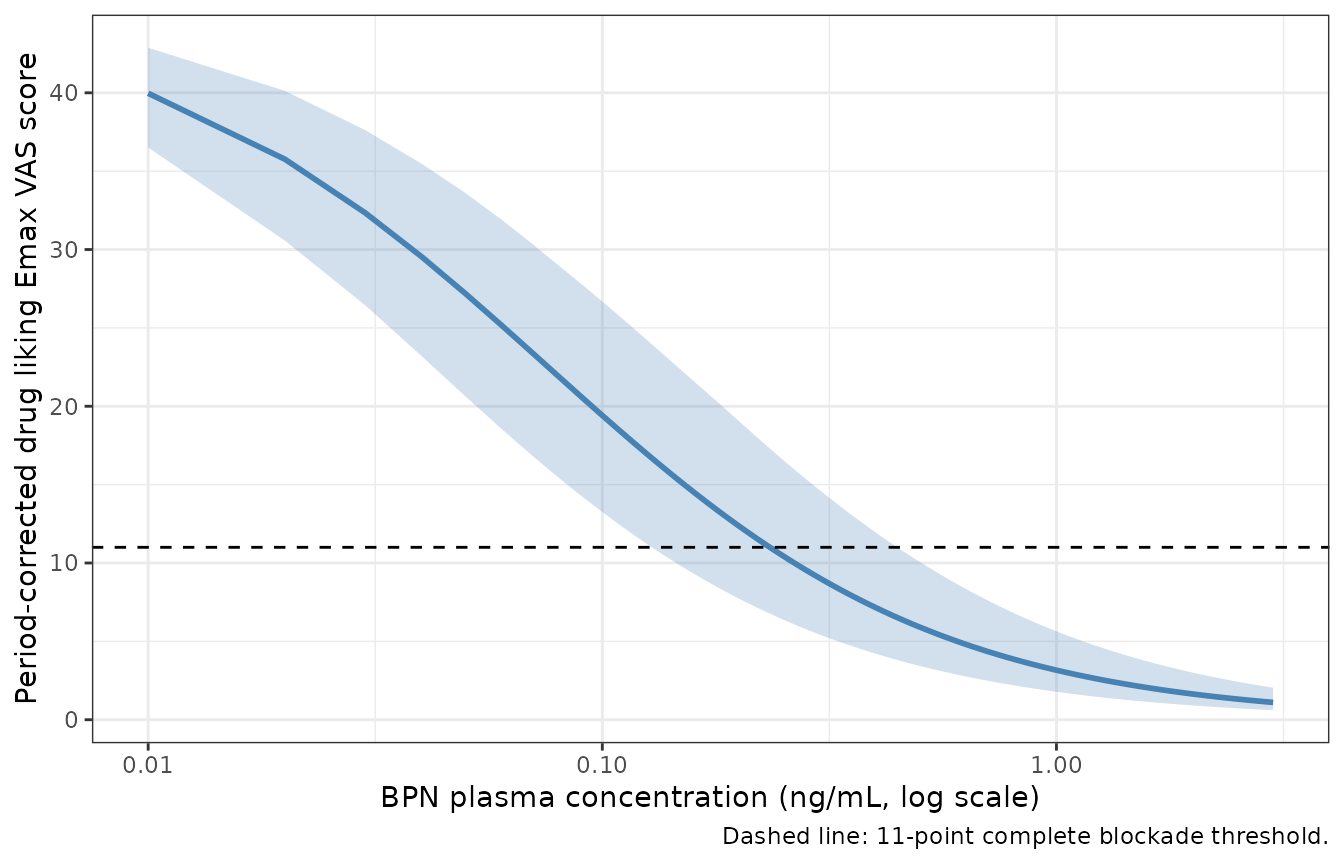
Replicates Figure 4 of Walsh 2024: period-corrected drug liking Emax VAS score versus BPN plasma concentration. The dashed line is the 11-point complete blockade threshold.
The paper’s headline clinical result is that drug liking is effectively blocked at a BPN plasma concentration of 0.4 ng/mL, defined as the concentration at which the upper 95% confidence limit of the simulated score falls below the 11-point threshold. That crossing is recovered below.
# which(...)[1] is NA when nothing crosses, and stopifnot(NA > 0.2) reports
# only "crossing > 0.2 is not TRUE", which says nothing about why. Fail on the
# empty case explicitly so the next person sees the actual problem.
below <- which(fig4$hi <= 11)
if (!length(below)) {
  stop("no concentration on the grid brings the upper 97.5% limit to <= 11 ",
       "points (min hi = ", signif(min(fig4$hi), 4), "); the uncertainty band ",
       "is wrong, not merely off-target")
}
crossing <- fig4$CP_BPN_NGML[below[1]]

tibble::tibble(
  Quantity = c(
    "Concentration where the upper 97.5% limit crosses 11 points",
    "Typical drug liking Emax VAS score at 0.4 ng/mL",
    "IC90 (drug liking)"
  ),
  Simulated = c(
    sprintf("%.3f ng/mL", crossing),
    sprintf("%.2f VAS units", fig4$typical[which.min(abs(fig4$CP_BPN_NGML - 0.4))]),
    "0.675 ng/mL"
  ),
  Published = c("0.4 ng/mL", "below the 11-point threshold", "0.675 ng/mL")
) |>
knitr::kable(caption = "Complete-blockade threshold (Walsh 2024 Figure 4).")| Quantity | Simulated | Published |
|---|---|---|
| Concentration where the upper 97.5% limit crosses 11 points | 0.450 ng/mL | 0.4 ng/mL |
| Typical drug liking Emax VAS score at 0.4 ng/mL | 7.15 VAS units | below the 11-point threshold |
| IC90 (drug liking) | 0.675 ng/mL | 0.675 ng/mL |
# The approximate uncertainty band should put the crossing near the paper's
# 0.4 ng/mL; allow a generous window because the covariance matrix is not
# published and only the diagonal RSEs are available.
stopifnot(crossing > 0.2, crossing < 0.8)
Replicating Supplementary Figure S7: COWS application
Supplementary Figure S7 simulates the COWS score across BPN plasma concentrations of 0-10 ng/mL including inter-individual variability, and reports the proportion of participants below the mild-withdrawal threshold of 5. The concentration sweep below uses 200 participants, the cohort cap for these vignettes; the single-concentration gate that follows it uses the paper’s own 1,000.
Because the published likelihood is a bounded integer model, the simulated continuous score is floored to an integer before the category proportions are computed.
n_sub <- 200L
cows_grid <- c(seq(0, 1, by = 0.02), seq(1.2, 10, by = 0.2))

cows_ev <- tidyr::expand_grid(
  id = seq_len(n_sub), time = seq_along(cows_grid)
) |>
  dplyr::mutate(CP_BPN_NGML = cows_grid[time], evid = 0L, amt = 0)

cows_sim <- rxode2::rxSolve(cows, cows_ev, returnType = "data.frame") |>
  dplyr::mutate(score = floor(sim))

cows_sum <- cows_sim |>
  dplyr::group_by(CP_BPN_NGML) |>
  dplyr::summarise(
    median = median(score),
    lo50 = quantile(score, 0.25, names = FALSE),
    hi50 = quantile(score, 0.75, names = FALSE),
    lo90 = quantile(score, 0.05, names = FALSE),
    hi90 = quantile(score, 0.95, names = FALSE),
    pct_below5 = 100 * mean(score < 5),
    .groups = "drop"
  )

ggplot2::ggplot(cows_sum, ggplot2::aes(x = CP_BPN_NGML)) +
  ggplot2::geom_ribbon(ggplot2::aes(ymin = lo90, ymax = hi90),
                       fill = "steelblue", alpha = 0.18) +
  ggplot2::geom_ribbon(ggplot2::aes(ymin = lo50, ymax = hi50),
                       fill = "steelblue", alpha = 0.35) +
  ggplot2::geom_line(ggplot2::aes(y = median), linewidth = 1) +
  ggplot2::geom_line(ggplot2::aes(y = pct_below5 * 44 / 100),
                     linetype = "dashed") +
  ggplot2::geom_hline(yintercept = 5, linetype = "dotted", colour = "red") +
  ggplot2::scale_y_continuous(
    name = "COWS total score",
    limits = c(0, 44),
    sec.axis = ggplot2::sec_axis(
      ~ . * 100 / 44,
      name = "Participants with COWS below 5 (%)"
    )
  ) +
  ggplot2::labs(
    x = "BPN plasma concentration (ng/mL)",
    caption = paste(
      "Solid: median. Shaded: 50% and 90% prediction intervals.",
      "Dashed: percent below 5. Dotted red: mild-withdrawal threshold."
    )
  ) +
  ggplot2::theme_bw()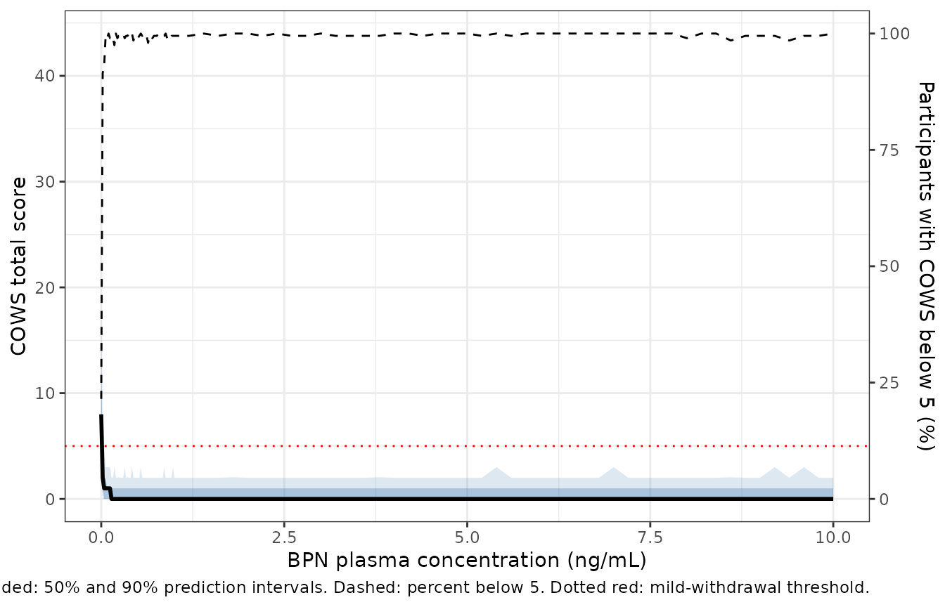
Replicates Supplementary Figure S7 of Walsh 2024: simulated COWS total score and the proportion of participants with COWS below 5, versus BPN plasma concentration.
The paper states that at a BPN plasma concentration of 0.100 ng/mL, 99.5% of simulated patients had a COWS score below 5 and 80.4% had a COWS score of 1 or less. Both are reproduced directly.
This single-concentration gate uses the paper’s own cohort size of 1,000 rather than the 200 used for the figure above. A proportion estimated from 200 draws has a standard error of roughly 3 percentage points, which is too coarse to resolve 80.4% and makes the comparison swing by ten points between renders; matching the published design removes that noise. The cost is negligible because this is a single time point with no ODE to integrate.
n_app <- 1000L

at_point <- rxode2::rxSolve(
  cows,
  data.frame(id = seq_len(n_app), time = 0, CP_BPN_NGML = 0.100,
             evid = 0L, amt = 0),
  returnType = "data.frame"
) |>
  dplyr::mutate(score = floor(sim))

binom_ci <- function(p, n, side) {
  half <- 1.96 * sqrt(p * (1 - p) / n)
  100 * if (side == "lo") max(0, p - half) else min(1, p + half)
}

p5 <- mean(at_point$score < 5)
p1 <- mean(at_point$score <= 1)

app <- tibble::tibble(
  Quantity = c("COWS below 5", "COWS of 1 or less"),
  `Simulated (%)` = round(100 * c(p5, p1), 1),
  `95% CI` = c(
    sprintf("%.1f to %.1f", binom_ci(p5, n_app, "lo"), binom_ci(p5, n_app, "hi")),
    sprintf("%.1f to %.1f", binom_ci(p1, n_app, "lo"), binom_ci(p1, n_app, "hi"))
  ),
  `Published (%)` = c(99.5, 80.4)
)

knitr::kable(
  app,
  caption = paste(
    "Gate: COWS category proportions at 0.100 ng/mL",
    "(Walsh 2024 Results / Supplementary Figure S7)."
  )
)| Quantity | Simulated (%) | 95% CI | Published (%) |
|---|---|---|---|
| COWS below 5 | 99.2 | 98.6 to 99.8 | 99.5 |
| COWS of 1 or less | 81.1 | 78.7 to 83.5 | 80.4 |
# Agreement is asserted to within 2 percentage points rather than by strict
# containment in the binomial interval. The packaged model is the CONTINUOUS
# relaxation of the published bounded-integer likelihood (see Assumptions), so
# a sub-percentage-point offset in a category proportion is expected and is not
# a defect; 2 points is still far tighter than any real encoding error, which
# would move these proportions by tens of points.
stopifnot(
  abs(100 * p5 - 99.5) < 2,
  abs(100 * p1 - 80.4) < 2
)
Endpoint sensitivity ordering
A qualitative result the paper emphasises in the Discussion is that drug liking requires a higher BPN concentration to suppress than either desire to use or withdrawal: the drug liking IC90 (0.675 ng/mL) is above the lowest observed BPN concentration in the study (0.636 ng/mL), whereas the desire to use and COWS IC90 values (0.116 and 0.109 ng/mL) are well below it.
tibble::tibble(
  Endpoint = c("Drug liking Emax VAS", "Desire to use VAS", "COWS total score"),
  `IC90 (ng/mL)` = c(0.675, 0.116, 0.109),
  `Below lowest observed BPN (0.636 ng/mL)` = c(FALSE, TRUE, TRUE)
) |>
knitr::kable(caption = "Endpoint sensitivity ordering (Walsh 2024 Discussion).")| Endpoint | IC90 (ng/mL) | Below lowest observed BPN (0.636 ng/mL) |
|---|---|---|
| Drug liking Emax VAS | 0.675 | FALSE |
| Desire to use VAS | 0.116 | TRUE |
| COWS total score | 0.109 | TRUE |
stopifnot(0.675 > 0.636, 0.116 < 0.636, 0.109 < 0.636)Assumptions and deviations
No PK model is packaged. Walsh 2024 does not report the CAM2038 popPK model, and no buprenorphine popPK model exists in
nlmixr2lib. All three models therefore requireCP_BPN_NGMLto be supplied per observation record from an external source. Users can digitise Supplementary Figure S2 of the paper for observed concentration-time profiles, or supply their own popPK simulation.No PKNCA analysis. These are PD-only algebraic models with no dosing and no concentration state, so non-compartmental analysis does not apply. The validation above uses the paper’s own reported exposure-response quantities instead.
Figure 4 uncertainty band is approximate. The paper drew 10,000 parameter sets from the estimated covariance matrix. Only the diagonal relative standard errors are published, so the band here draws 200 sets from independent log-normal distributions and ignores the correlation between
BaselineandIC50. The resulting complete-blockade crossing (approximately 0.4 ng/mL) agrees with the paper, but the band width should not be read as an exact reproduction.Bounded-integer flooring is applied in the vignette, not the model. The published COWS likelihood is a bounded integer model, in which the latent probit-scale prediction is mapped through the normal CDF and then floored to one of 45 ordered categories.
rxode2has no bounded-integer residual family, soWalsh_2024_buprenorphine_cowsencodes the continuous relaxationprobitNorm(addSd, 0, 45), which is the same construction without the flooring step. Reproducing the paper’s category proportions requiresfloor()on the simulated score, as done above. Individual-level predictions from the packaged model are therefore continuous, not integer.COWS latent-to-observable back-transform. The paper’s
IPREDfor COWS is defined on the scale of the standard-normal quantile function, whereasrxode2’sprobitNorm(sd, low, hi)expects the prediction on the observed scale. The model file therefore maps the latent value throughprobitInv(latent, 0, 45), which is the exact inverse of the transformprobitNormapplies internally, so the residual error still lands on the paper’s quantile scale. Feeding the latent value directly toprobitNormwould put the argument outside the (0, 45) bounds and silently returnNA.Table S3 heads its variability column “CV”. The tabulated quantities are standard deviations, not coefficients of variation. Two things establish this: the Supplementary Methods describe IIV in exponential form
P_i = TVP * exp(eta_i)witheta_i ~ N(0, omega^2), whose natural reporting quantity isomega; and the same column carries the RUV entry (0.783), which is additive on the logit scale and so has no coefficient-of-variation interpretation at all. Its value is also near-identical to the drug liking model’s additive logit-scale RUV (0.744), which Table 1 explicitly labels “SD”. The values are squared to give the variancesrxode2expects.COWS IIV correlation is retained as reported. Table S4 gives the correlation between the
BASEb.intandLBASEb.intrandom effects as 0.0203 with an RSE of 478%, i.e. indistinguishable from zero. The off-diagonal is reconstructed ascorr * omega_1 * omega_2 = 0.0203 * 0.454 * 0.0948and retained rather than dropped, so the packaged model matches the published table.The two COWS random effects enter differently. The Supplementary Methods specify “additive IIV on BASEb.int., exponential IIV on LBASEb.int.” The model file follows this exactly (
probitbase + etaprobitbaseversusprobitbase_low * exp(etaprobitbase_low)); exponential IIV on a negative parameter scales its magnitude while preserving its sign, keeping the lower asymptote a lower asymptote.Drug liking period-correction direction. The Methods section states the score was period-corrected “whereby the post-hydromorphone challenge score was subtracted from the prechallenge value”, which would make the endpoint negative. The Figure 3 caption states the opposite and correct direction: “the pre-challenge value was subtracted from the maximum value recorded after each 18 mg hydromorphone challenge”. The positive baseline of 45.3 VAS units in Table 1 confirms the Figure 3 caption, so the Methods sentence is treated as an author slip and the model encodes post minus pre.
Covariates were screened but not retained. Age, sex, ethnicity, race, body weight, height and BMI were tested on the drug liking IC50 by a single forward step in PsN stepwise covariate modelling; none was significant (p > 0.2) and the paper reports no point estimates. They are recorded in the model file under
covariatesDataExcludedto preserve the provenance of the screen without adding unused covariates to the model. No covariate analysis is reported for the desire to use or COWS endpoints.IIV on Imax is fixed to zero. Table 1 reports
IIV Imaxas SD = 0 (FIX) for drug liking, so no random effect is placed onimax.Arm sizes. Table S1 reports 22 participants on 24 mg and 25 on 32 mg. The Figure 1 caption gives “32 mg: n = 24”, which refers to the PK-evaluable subset; the model files use the Table S1 values.