Lipid-lowering therapy MACE-component MBMA (Volkova 2023)
Source:vignettes/articles/Volkova_2023_lipidLowering_mace_mbma.Rmd
Volkova_2023_lipidLowering_mace_mbma.RmdModel and source
- Citation: Volkova A, Shulgin B, Helmlinger G, Peskov K, Sokolov V. Optimization of the MACE endpoint composition to increase power in studies of lipid-lowering therapies - a model-based meta-analysis. Front Cardiovasc Med. 2023;10:1242845 (published online 08 January 2024). doi:10.3389/fcvm.2023.1242845.
- Article (open access): https://doi.org/10.3389/fcvm.2023.1242845
Volkova 2023 is a model-based meta-analysis (MBMA) of 54 randomised controlled trials of lipid-lowering therapy. Its purpose is not to describe pharmacokinetics but to answer a trial-design question: given a planned population and an achievable LDL-C reduction, which combination of individual cardiovascular events should a composite MACE endpoint contain in order to reach statistical significance with the smallest enrolment?
The paper answers that in two steps, and the packaged model implements both:
- A random-effects meta-regression per individual event, predicting the trial-level treatment effect (log risk ratio versus comparator) from therapy class and trial-level population characteristics.
- A sample-size calculator that converts an effect size and a control-arm event rate into the minimum enrolment needed for the upper bound of the 95% confidence interval on log(RR) to fall below zero.
mod <- readModelDb("Volkova_2023_lipidLowering_mace_mbma")Population
The pooled dataset is 270,471 patients across 54 trials (47 statin, 7 anti-PCSK9), with mean age 61.2 years, 30.3% women and a mean baseline LDL-C of 136.6 mg/dL. Trials shorter than 1.5 years of cardiovascular follow-up, or with fewer than 100 participants per treatment group, were excluded; follow-up ranged from 1.5 to 10 years (mean 3.87).
Fifteen trials enrolled primary-prevention populations, 21 were secondary-prevention studies and 18 enrolled mixed or unstated populations. Six of 54 trials admitted patients with severe renal disease.
Every observation is a trial, not a patient. The dependent variable is a risk ratio computed from per-arm event and subject counts, and the covariates are trial-level aggregates (mean age, percent hypertensive, mean baseline HDL-C). The model therefore predicts a trial-level mean treatment effect, and must not be read as an individual patient’s risk.
The full metadata is available programmatically:
str(rxode2::rxode(readModelDb("Volkova_2023_lipidLowering_mace_mbma"))$population)
#> List of 15
#>  $ species           : chr "human"
#>  $ n_subjects        : int 270471
#>  $ n_studies         : int 54
#>  $ age_range         : chr "Trial-level mean age 49.75-75.35 years (mean of means 61.2, SD 4.9) across the 54 trials (Volkova 2023 Supplementary Table 3)."
#>  $ weight_range      : chr "Body weight was not collected; body mass index was, with trial-level means 23.5-30.15 kg/m^2 (mean 26.89, SD 1."| __truncated__
#>  $ sex_female_pct    : num 30.3
#>  $ disease_state     : chr "Dyslipidemia / hypercholesterolemia, treated with a statin or an anti-PCSK9 agent against a placebo or standard"| __truncated__
#>  $ dose_range        : chr "Trial-level; dose and dose schedule were digitised per cohort but dose itself was NOT a covariate in any final "| __truncated__
#>  $ regions           : chr "Multinational; 54 randomised controlled trials published in English and indexed in PubMed or ClinicalTrials.gov"| __truncated__
#>  $ baseline_lipids   : chr "Trial-level baseline means (Volkova 2023 Supplementary Table 3): LDL-C 136.57 mg/dL (SD 27.71; range 87.9-195.5"| __truncated__
#>  $ treatment_response: chr "Trial-level comparator-adjusted changes (Volkova 2023 Supplementary Table 3): delta-LDL-C -36.91 mg/dL (SD 16.5"| __truncated__
#>  $ follow_up         : chr "1.5-10 years (mean 3.87, SD 1.83). Trials with mean cardiovascular follow-up shorter than 1.5 years, or fewer t"| __truncated__
#>  $ therapy_split     : chr "47 statin trials and 7 anti-PCSK9 trials (evolocumab, alirocumab, bococizumab, inclisiran)."
#>  $ other_demographics: chr "Trial-level means (Volkova 2023 Supplementary Table 3): males 69.73%, hypertension 54.71%, diabetes 22.72%, smo"| __truncated__
#>  $ notes             : chr "Study-level (aggregate) meta-analytic data only -- no individual patient data. Each observation is a trial-leve"| __truncated__
Trial-level covariate distributions, used below to build a plausible design grid, are from Volkova 2023 Supplementary Table 3:
| Trial-level covariate | Mean | SD | Minimum | Maximum |
|---|---|---|---|---|
| Age (years) | 61.20 | 4.90 | 49.75 | 75.35 |
| Hypertension (%) | 54.71 | 22.61 | 15.70 | 100.00 |
| Baseline LDL-C (mg/dL) | 136.57 | 27.71 | 87.90 | 195.56 |
| Baseline HDL-C (mg/dL) | 45.82 | 6.05 | 35.96 | 59.55 |
| Baseline remnant-C (mg/dL) | 30.72 | 7.06 | 13.05 | 60.00 |
| delta-LDL-C (mg/dL) | -36.91 | 16.57 | -75.00 | 1.40 |
| Follow-up (years) | 3.87 | 1.83 | 1.50 | 10.00 |
Scope of this extraction
Volkova 2023 screened 15 individual MACE components. Ten of them retained at least one covariate and are reported with full coefficients and standard errors in Table 1; those ten are implemented here:
| Implemented | Covariate retained |
|---|---|
| CR – coronary revascularization | delta-LDL-C |
| CM – coronary mortality | delta-LDL-C |
| nfMI – nonfatal myocardial infarction | delta-LDL-C, x renal-disease interaction |
| CVM – cardiovascular mortality | baseline HDL-C |
| MI – myocardial infarction (all) | baseline HDL-C |
| TM – total (all-cause) mortality | baseline HDL-C |
| HF – heart failure | baseline remnant cholesterol |
| iST – ischemic stroke | hypertension prevalence |
| fST – fatal stroke | renal-disease enrolment |
| ST – stroke (unspecified) | prevention category x mean age |
The remaining five components (fMI, hST, nfST, TIA, UA) retained no covariate at any step of the search (Volkova 2023 Supplementary Table 4), so their final models are therapy-only. Those therapy-only effect sizes appear only as points in the Figure 2 forest plot – no numeric coefficient or standard error for them is printed anywhere in the paper or its supplement. They are therefore out of scope; see Errata.
The composite MACE endpoint itself was dropped by the authors before any modelling, because the Egger test found significant publication bias (p < 0.001) for it alone.
Source trace
Every ini() entry carries an in-file comment naming its
source location in
inst/modeldb/therapeuticArea/Volkova_2023_lipidLowering_mace_mbma.R.
The table below collects them, with the published standard errors that
the paper’s uncertainty propagation (Section 2.4) requires.
| Parameter | Estimate | SE | Source location (Volkova 2023) |
|---|---|---|---|
| int_cr | -0.035 | 0.057 | Table 1, CR beta_0 |
| e_pcsk9_cr | 0.220 | 0.067 | Table 1, CR beta_1 |
| e_dldlc_cr | 0.007 | 0.002 | Table 1, CR beta_2 |
| int_cvm | -0.625 | 0.253 | Table 1, CVM beta_0 |
| e_pcsk9_cvm | 0.082 | 0.067 | Table 1, CVM beta_1 |
| e_hdlc_cvm | 0.012 | 0.006 | Table 1, CVM beta_2 |
| int_hf | 0.554 | 0.253 | Table 1, HF beta_0 |
| e_pcsk9_hf | 0.097 | 0.111 | Table 1, HF beta_1 |
| e_remc_hf | -0.023 | 0.009 | Table 1, HF beta_2 |
| int_ist | -0.791 | 0.170 | Table 1, iST beta_0 |
| e_pcsk9_ist | -0.309 | 0.122 | Table 1, iST beta_1 |
| e_hypert_ist | 0.011 | 0.003 | Table 1, iST beta_2 |
| int_mi | 0.407 | 0.323 | Table 1, MI beta_0 |
| e_pcsk9_mi | 0.033 | 0.104 | Table 1, MI beta_1 |
| e_hdlc_mi | -0.017 | 0.008 | Table 1, MI beta_2 |
| int_st | -0.773 | 0.403 | Table 1, ST beta_0 |
| e_pcsk9_st | -0.056 | 0.096 | Table 1, ST beta_1 |
| e_age_st_primary | 0.007 | 0.007 | Table 1, ST beta_2 (Primary) |
| e_age_st_secondary | 0.010 | 0.006 | Table 1, ST beta_2 (Secondary) |
| e_age_st_mixed | 0.011 | 0.006 | Table 1, ST beta_2 (Both) |
| int_tm | -0.448 | 0.170 | Table 1, TM beta_0 |
| e_pcsk9_tm | 0.029 | 0.063 | Table 1, TM beta_1 |
| e_hdlc_tm | 0.008 | 0.004 | Table 1, TM beta_2 |
| int_cm | -0.019 | 0.064 | Table 1, CM beta_0 |
| e_pcsk9_cm | 0.147 | 0.109 | Table 1, CM beta_1 |
| e_dldlc_cm | 0.004 | 0.002 | Table 1, CM beta_2 |
| int_fst | -0.113 | 0.089 | Table 1, fST beta_0 |
| e_pcsk9_fst | 0.050 | 0.289 | Table 1, fST beta_1 |
| e_rd_fst | 0.654 | 0.283 | Table 1, fST beta_2 |
| int_nfmi | -0.057 | 0.091 | Table 1, nfMI beta_0 |
| e_pcsk9_nfmi | 0.242 | 0.100 | Table 1, nfMI beta_1 |
| e_dldlc_nfmi | 0.008 | 0.003 | Table 1, nfMI beta_2 |
| e_rd_dldlc_nfmi | -0.005 | 0.002 | Table 1, nfMI beta_3 |
| z975 | 1.960 | NA | Section 2.4 / Supplementary File 2 (fixed constant) |
The non-parameter equations are:
The sample-size formula (Section 2.4, derived in Supplementary File 2)
and the composite-endpoint aggregation (Supplementary File 3)
Note on transcription: the article PDF sets every negative number in
Table 1 with a Unicode minus sign (U+2212) rather than an ASCII hyphen,
and the same character is used for the leading minus of the
-4k term in the Section 2.4 display equation. Both were
confirmed against the supplement, where Supplementary File 2 derives the
formula step by step from the 2x2 event table, and independently against
the paper’s own published sample sizes (below).
Errata
No erratum, corrigendum or expression of concern was located for
Volkova 2023. Crossref reports no relation records against
DOI 10.3389/fcvm.2023.1242845; the Frontiers article landing page
carries no correction notice.
The article is dated 2023 by its DOI, journal volume (10) and Europe
PMC pubYear, but was published online on 08 January 2024
and its own citation block reads “(2024)”. The file stem uses 2023 to
match the DOI and index year; the reference field records
both.
Four discrepancies internal to the paper are recorded here.
The Results sentence labelled “MI” means nfMI. Section 3.2 states “For CR and MI, mean treatment benefit was decreased, respectively, by 24.6% [95% CI, 9.3-42.1] and 27.4% [95% CI, 4.7-55] in anti-PCSK9 treated populations.” The 27.4% figure is
exp(0.242) = 1.274, which is the nfMI beta_1; the MI beta_1 of 0.033 gives only 3.4%. The preceding paragraph of the same section confirms it, saying the therapy difference “was established only for CR and nfMI”. Table 1 is authoritative and is what the model encodes.Supplementary Table 3’s lipid subsection headings are transposed. The block headed “Baseline lipid measurements” contains the comparator-adjusted delta values, and the block headed “Treatment-related lipid measurements” contains the baseline values. The tell is that the latter block’s LDL-C mean of 136.57 mg/dL is the same number the main-text Results calls “mean baseline LDLc level of 136.6 mg/dl”. The model uses baseline HDL-C and baseline remnant cholesterol from that second block, per Table 1’s covariate labels.
The heart-failure narrative is a loose paraphrase. Section 3.2 says “an increase of 13 mg/dl in baseline remC resulted in an approximately 2-fold decrease in the RR of HF”. Taken literally that would need a coefficient near -0.053; Table 1 gives -0.023, for which a 13 mg/dL increase multiplies the risk ratio by
exp(-0.299) = 0.74. What does roughly double over 13 mg/dL is the risk reduction1 - RR: starting from the population mean remnant cholesterol of 30.72 mg/dL it goes from 14.1% to 36.3%. The quantified checks below reproduce eight other published contrasts exactly from Table 1, so Table 1 is treated as authoritative and the narrative sentence as imprecise.The Table 1 p-value column is not consistent with its own estimates and standard errors. Under a normal reference, iST beta_0 of -0.791 with SE 0.170 gives z = -4.65 and p ~ 3e-6, against a printed p = 0.01; several other rows disagree in the same direction. The likeliest cause is the pooling of 100 multiple imputations by Rubin’s rules, which replaces the normal reference with a t distribution on fractional degrees of freedom. The estimates and standard errors are confirmed exactly by the reproductions below and are what the model uses; the p-value column is not used and should not be relied on.
Two scope decisions:
Five therapy-only endpoints omitted. fMI, hST, nfST, TIA and UA retained no covariate, and their therapy-only effect sizes are shown only as points in the Figure 2 forest plot. Reading a point estimate and a standard error off a 330-pixel-wide forest plot for five endpoints and two therapy classes would inject twenty digitised numbers into a model whose value is its provenance, so they are left out rather than estimated by eye. The practical consequence is that the paper’s own illustrative 3-point MACE (nfMI + nfST + CVM) cannot be assembled from this model alone, because nfST is one of the five. The composite machinery is still demonstrated below on the 4-point-style combination the paper found most efficient among endpoints this model does carry.
Control-arm event rates are an input, not an output. Volkova 2023 fitted a separate meta-regression of control-arm event rates against follow-up duration, but reported it only as fitted lines in Supplementary Figure 1; no coefficients are printed.
K_CTRLis therefore supplied externally. This is recoverable in practice, and the section below recovers it for nfMI by inverting the paper’s own published sample sizes.No between-study variance is encoded. These are random-effects meta-regressions, and the paper reports I-squared up to 48% for four endpoints, but it does not report tau-squared per endpoint anywhere. Rather than invent a variance, the model carries typical values only. Predictions are the meta-regression mean, without residual between-trial heterogeneity.
Trial-level design grid
The “virtual cohort” for a study-level MBMA is a grid of trial designs, not of patients. Each row is one hypothetical trial. Values are anchored to the Supplementary Table 3 distributions above.
# A reference trial: population means from Supplementary Table 3.
ref_trial <- list(
  TRT_PCSK9I         = 0,        # statin (the Table 1 reference class)
  LDLC_DELTA         = -36.91,   # mg/dL, comparator-adjusted
  HDLC               = 45.82,    # mg/dL, baseline
  REMC               = 30.72,    # mg/dL, baseline
  DIS_HYPERT_PERCENT = 54.71,    # percent
  RENALIMP_SEV       = 0,        # trial excluded severe renal disease
  PREVENT_PRIMARY    = 0,
  PREVENT_SECONDARY  = 1,
  PREVENT_MIXED      = 0,
  AGE                = 61.2,     # years
  LOGRR_TARGET       = -0.3,     # placeholder; overridden where N is computed
  K_CTRL             = 0.05      # placeholder; overridden where N is computed
)

#' Build an rxode2 event frame of trial scenarios.
#'
#' Each row is one trial design; `evid = 0` marks it as an observation
#' record so rxode2 evaluates the algebraic model at that covariate set.
#' Any element of `ref_trial` not overridden in `...` is held at its
#' population-mean value.
make_trials <- function(...) {
  overrides <- list(...)
  stopifnot(all(names(overrides) %in% names(ref_trial)))
  n <- if (length(overrides)) max(lengths(overrides)) else 1L
  out <- lapply(ref_trial, function(v) rep(v, length.out = n))
  for (nm in names(overrides)) out[[nm]] <- rep(overrides[[nm]], length.out = n)
  out <- as.data.frame(out)
  out$id <- seq_len(n)
  out$time <- 0
  out$evid <- 0L
  out
}

cov_names <- names(ref_trial)

#' Solve the algebraic MBMA over a frame of trial scenarios.
solve_trials <- function(events) {
  rxode2::rxSolve(mod, events = events, keep = cov_names) |>
    as.data.frame()
}
Replication: LDL-C-driven endpoints
Three endpoints – coronary revascularization, coronary mortality and nonfatal myocardial infarction – take the comparator-adjusted LDL-C change as their covariate. Volkova 2023 Figure 3 sweeps delta-LDL-C from -10 to -75 mg/dL; the same range is used here.
dldlc_grid <- seq(-75, -10, by = 1)

sim_ldlc <- dplyr::bind_rows(
  solve_trials(make_trials(LDLC_DELTA = dldlc_grid, TRT_PCSK9I = 0)),
  solve_trials(make_trials(LDLC_DELTA = dldlc_grid, TRT_PCSK9I = 1))
)

sim_ldlc |>
  dplyr::select(LDLC_DELTA, TRT_PCSK9I, rr_cr, rr_cm, rr_nfmi) |>
  tidyr::pivot_longer(c(rr_cr, rr_cm, rr_nfmi),
                      names_to = "endpoint", values_to = "rr") |>
  dplyr::mutate(
    endpoint = dplyr::recode(endpoint,
      rr_cr = "CR (coronary revascularization)",
      rr_cm = "CM (coronary mortality)",
      rr_nfmi = "nfMI (nonfatal MI)"),
    Therapy = ifelse(TRT_PCSK9I == 1, "anti-PCSK9", "statin")
  ) |>
  ggplot(aes(x = LDLC_DELTA, y = rr, colour = Therapy)) +
  geom_line(linewidth = 0.9) +
  geom_hline(yintercept = 1, linetype = "dashed") +
  facet_wrap(~endpoint) +
  scale_x_continuous(name = "Comparator-adjusted change in LDL-C (mg/dL)") +
  scale_y_continuous(name = "Risk ratio vs comparator") +
  theme_bw() +
  theme(legend.position = "bottom")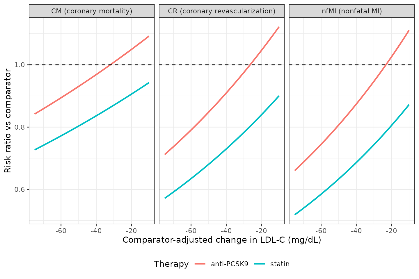
Predicted risk ratio versus comparator-adjusted LDL-C lowering for the three LDL-C-driven MACE components, by therapy class. Reproduces the effect-size layer underlying Volkova 2023 Figure 3.
The anti-PCSK9 curves sit above the statin curves for CR and nfMI: after adjusting for the LDL-C reduction actually achieved, anti-PCSK9 therapy delivered less benefit on these two endpoints than a statin achieving the same LDL-C lowering. That is the paper’s central mechanistic observation, which it attributes to statin pleiotropy.
Replication: baseline-HDL-C-driven endpoints
Baseline HDL-C enters three endpoints, and the sign is not the same for all three – higher baseline HDL-C predicts less benefit for total and cardiovascular mortality but more benefit for myocardial infarction.
hdlc_grid <- seq(36, 60, by = 0.5)   # Supplementary Table 3 observed range

sim_hdlc <- solve_trials(make_trials(HDLC = hdlc_grid, TRT_PCSK9I = 0))

sim_hdlc |>
  dplyr::select(HDLC, rr_cvm, rr_mi, rr_tm) |>
  tidyr::pivot_longer(c(rr_cvm, rr_mi, rr_tm),
                      names_to = "endpoint", values_to = "rr") |>
  dplyr::mutate(endpoint = dplyr::recode(endpoint,
    rr_cvm = "CVM (cardiovascular mortality)",
    rr_mi  = "MI (myocardial infarction)",
    rr_tm  = "TM (total mortality)")) |>
  ggplot(aes(x = HDLC, y = rr, colour = endpoint)) +
  geom_line(linewidth = 0.9) +
  geom_hline(yintercept = 1, linetype = "dashed") +
  scale_x_continuous(name = "Trial-level baseline HDL-C (mg/dL)") +
  scale_y_continuous(name = "Risk ratio vs comparator") +
  labs(colour = NULL) +
  theme_bw() +
  theme(legend.position = "bottom")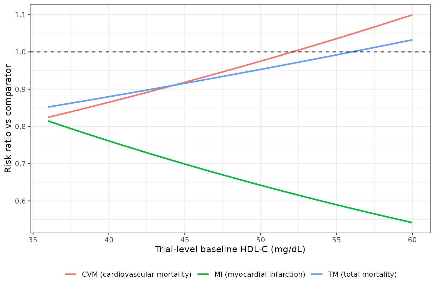
Predicted risk ratio versus trial-level baseline HDL-C for the three HDL-C-driven MACE components (statin trials). The dashed line is RR = 1; where a curve crosses it, the model predicts no treatment benefit.
Volkova 2023 Section 3.2 states that “populations with baseline HDLc above 48 mg/dl for statin treatment … were shown to lack any significant response in RR of TM and CVM”. The model’s own crossing points bracket that value:
# HDL-C at which each mortality endpoint's predicted RR reaches 1
# (statin trials): solve int + e_hdlc * HDLC = 0.
hdlc_cross <- tibble::tibble(
  endpoint = c("CVM", "TM"),
  crossing_mgdl = c(0.625 / 0.012, 0.448 / 0.008)
)
hdlc_cross
#> # A tibble: 2 × 2
#>   endpoint crossing_mgdl
#>   <chr>            <dbl>
#> 1 CVM               52.1
#> 2 TM                56

stopifnot(
  # Both crossings sit within a few mg/dL of the paper's stated 48 mg/dL
  # threshold, on either side of it. Deterministic algebra, so this is an
  # exact statement about the encoded coefficients.
  all(abs(hdlc_cross$crossing_mgdl - 48) < 10),
  hdlc_cross$crossing_mgdl[1] > 48,   # CVM crosses above 48
  hdlc_cross$crossing_mgdl[2] > 48    # TM  crosses above 48
)
Replication: stroke, prevention category x age
The unspecified-stroke model is the only one with an interaction between two population descriptors and no main effect for either: mean age carries a prevention-category-specific slope.
age_grid <- seq(50, 76, by = 0.5)

sim_st <- dplyr::bind_rows(
  solve_trials(make_trials(AGE = age_grid, PREVENT_PRIMARY = 1,
                           PREVENT_SECONDARY = 0, TRT_PCSK9I = 0)),
  solve_trials(make_trials(AGE = age_grid, PREVENT_PRIMARY = 0,
                           PREVENT_SECONDARY = 1, TRT_PCSK9I = 0)),
  solve_trials(make_trials(AGE = age_grid, PREVENT_PRIMARY = 1,
                           PREVENT_SECONDARY = 0, TRT_PCSK9I = 1)),
  solve_trials(make_trials(AGE = age_grid, PREVENT_PRIMARY = 0,
                           PREVENT_SECONDARY = 1, TRT_PCSK9I = 1))
) |>
  dplyr::mutate(
    Prevention = ifelse(PREVENT_PRIMARY == 1, "primary", "secondary"),
    Therapy    = ifelse(TRT_PCSK9I == 1, "anti-PCSK9", "statin")
  )

published_st <- tibble::tibble(
  Prevention = c("primary", "secondary", "primary", "secondary"),
  Therapy    = c("statin", "statin", "anti-PCSK9", "anti-PCSK9"),
  AGE        = 60,
  rr_pub     = c(0.71, 0.82, 0.67, 0.78)
)

ggplot(sim_st, aes(x = AGE, y = rr_st, colour = Prevention,
                   linetype = Therapy)) +
  geom_line(linewidth = 0.9) +
  geom_point(data = published_st, aes(y = rr_pub), size = 2.5,
             inherit.aes = TRUE, show.legend = FALSE) +
  scale_x_continuous(name = "Trial-level mean age (years)") +
  scale_y_continuous(name = "Stroke risk ratio vs comparator") +
  theme_bw() +
  theme(legend.position = "bottom")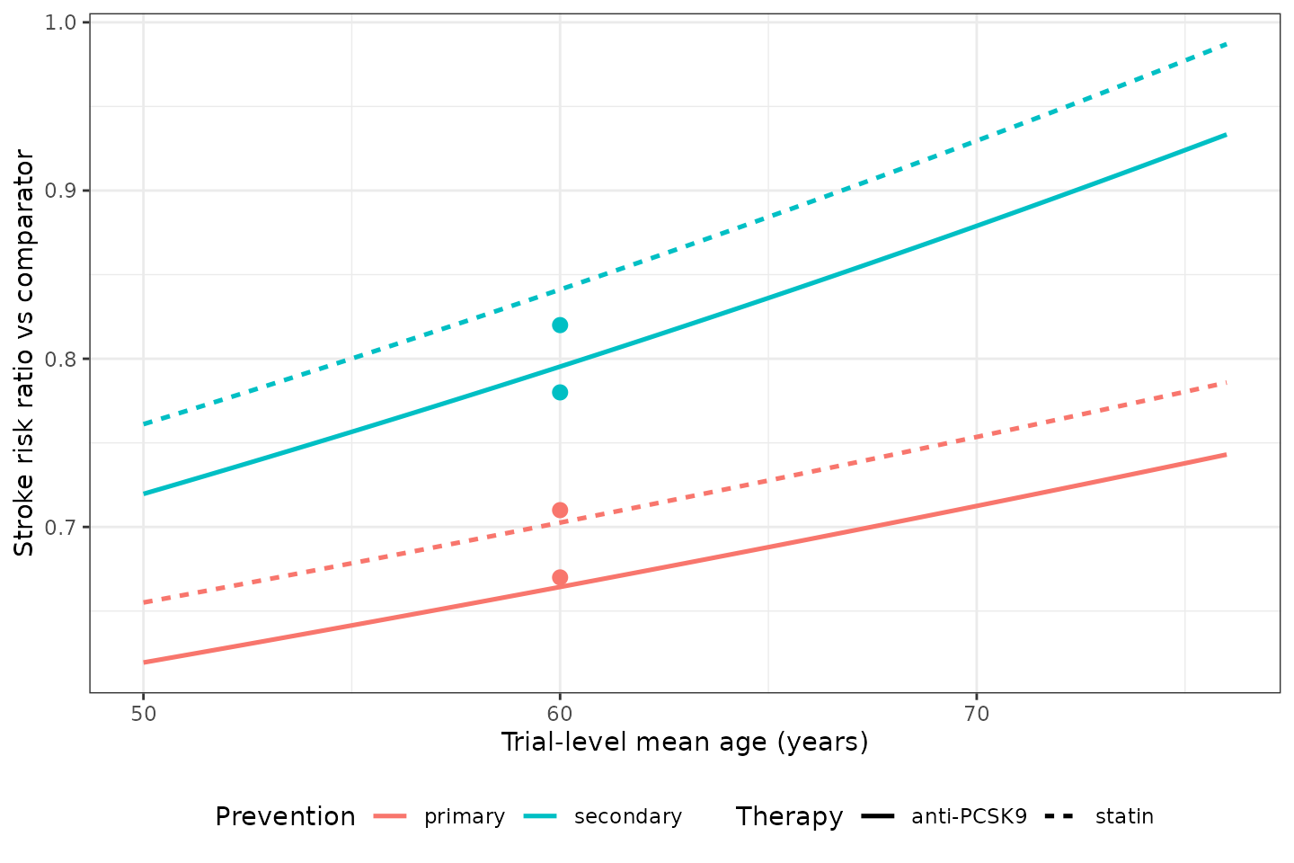
Predicted stroke risk ratio versus trial-level mean age, by prevention category and therapy class. Points mark the four values quoted in Volkova 2023 Section 3.2 for a mean age of 60 years.
Validation against published numerical anchors
Volkova 2023 is not a pharmacokinetic model, so a PKNCA non-compartmental analysis is not the right validation – there is no concentration-time profile to integrate. Instead the model is checked against every quantitative contrast the paper states in prose, each of which is an independent restatement of Table 1 coefficients.
mmol <- 38.67   # mg/dL per 1 mmol/L of cholesterol (Volkova 2023 Section 3.2)

# --- 1. Effect of a 1 mmol/L LDL-C reduction, by endpoint --------------
base_ldl <- solve_trials(make_trials(LDLC_DELTA = 0, RENALIMP_SEV = 0))
drop_ldl <- solve_trials(make_trials(LDLC_DELTA = -mmol, RENALIMP_SEV = 0))
drop_rd  <- solve_trials(make_trials(LDLC_DELTA = -mmol, RENALIMP_SEV = 1))

ldl_anchors <- tibble::tibble(
  anchor = c("CR", "CM", "nfMI", "nfMI, trial enrolling severe renal disease"),
  model_pct = 100 * c(
    drop_ldl$rr_cr   / base_ldl$rr_cr   - 1,
    drop_ldl$rr_cm   / base_ldl$rr_cm   - 1,
    drop_ldl$rr_nfmi / base_ldl$rr_nfmi - 1,
    drop_rd$rr_nfmi  / solve_trials(make_trials(LDLC_DELTA = 0,
                                                RENALIMP_SEV = 1))$rr_nfmi - 1
  ),
  published_pct = c(-24, -14, -27, -11)
)

# --- 2. Anti-PCSK9 vs statin, CR and nfMI ------------------------------
statin <- solve_trials(make_trials(TRT_PCSK9I = 0))
pcsk9  <- solve_trials(make_trials(TRT_PCSK9I = 1))

pcsk9_anchors <- tibble::tibble(
  anchor = c("CR: anti-PCSK9 vs statin", "nfMI: anti-PCSK9 vs statin"),
  model_pct = 100 * c(pcsk9$rr_cr / statin$rr_cr - 1,
                      pcsk9$rr_nfmi / statin$rr_nfmi - 1),
  published_pct = c(24.6, 27.4)
)

# --- 3. Ratio-scale contrasts (iST hypertension, fST renal disease) ----
ht25 <- solve_trials(make_trials(DIS_HYPERT_PERCENT = 25))
ht75 <- solve_trials(make_trials(DIS_HYPERT_PERCENT = 75))
rd0  <- solve_trials(make_trials(RENALIMP_SEV = 0))
rd1  <- solve_trials(make_trials(RENALIMP_SEV = 1))

ratio_anchors <- tibble::tibble(
  anchor = c("iST: 75% vs 25% hypertensive population",
             "fST: trial enrolling severe renal disease vs not"),
  model_ratio = c(ht75$rr_ist / ht25$rr_ist, rd1$rr_fst / rd0$rr_fst),
  published_ratio = c(1.7, 1.9)
)

# --- 4. Stroke risk ratios at mean age 60 ------------------------------
st_anchors <- published_st |>
  dplyr::mutate(model_rr = c(
    solve_trials(make_trials(AGE = 60, PREVENT_PRIMARY = 1,
                             PREVENT_SECONDARY = 0, TRT_PCSK9I = 0))$rr_st,
    solve_trials(make_trials(AGE = 60, PREVENT_PRIMARY = 0,
                             PREVENT_SECONDARY = 1, TRT_PCSK9I = 0))$rr_st,
    solve_trials(make_trials(AGE = 60, PREVENT_PRIMARY = 1,
                             PREVENT_SECONDARY = 0, TRT_PCSK9I = 1))$rr_st,
    solve_trials(make_trials(AGE = 60, PREVENT_PRIMARY = 0,
                             PREVENT_SECONDARY = 1, TRT_PCSK9I = 1))$rr_st
))| Published contrast (Volkova 2023 Section 3.2) | Model | Paper |
|---|---|---|
| CR | -23.7% | -24% |
| CM | -14.3% | -14% |
| nfMI | -26.6% | -27% |
| nfMI, trial enrolling severe renal disease | -11.0% | -11% |
| CR: anti-PCSK9 vs statin | +24.6% | +24.6% |
| nfMI: anti-PCSK9 vs statin | +27.4% | +27.4% |
| iST: 75% vs 25% hypertensive population | 1.73-fold | 1.7-fold |
| fST: trial enrolling severe renal disease vs not | 1.92-fold | 1.9-fold |
| ST at age 60: statin, primary | RR 0.703 | RR 0.71 |
| ST at age 60: statin, secondary | RR 0.841 | RR 0.82 |
| ST at age 60: anti-PCSK9, primary | RR 0.664 | RR 0.67 |
| ST at age 60: anti-PCSK9, secondary | RR 0.795 | RR 0.78 |
stopifnot(
  # Guard first: an empty tibble would make every all() below vacuously TRUE.
  nrow(ldl_anchors) == 4L, nrow(pcsk9_anchors) == 2L,
  nrow(ratio_anchors) == 2L, nrow(st_anchors) == 4L,
  !anyNA(c(ldl_anchors$model_pct, pcsk9_anchors$model_pct,
           ratio_anchors$model_ratio, st_anchors$model_rr)),

  # The model is deterministic and the comparison is against the paper's own
  # rounded restatements of Table 1, so tolerances are set by the paper's
  # printed precision, not by simulation noise.

  # Percentage-change anchors: the paper prints whole percentages.
  all(abs(ldl_anchors$model_pct - ldl_anchors$published_pct) < 0.7),
  # Anti-PCSK9 contrasts: printed to one decimal, and both reproduce to it.
  all(abs(pcsk9_anchors$model_pct - pcsk9_anchors$published_pct) < 0.1),
  # Fold-change anchors: printed to one decimal.
  all(abs(ratio_anchors$model_ratio - ratio_anchors$published_ratio) < 0.05),
  # Stroke risk ratios: printed to two decimals; the largest gap comes from
  # the secondary-prevention slope being printed as 0.010 (3 dp).
  all(abs(st_anchors$model_rr - st_anchors$rr_pub) < 0.025)
)
All published contrasts reproduce. The two anti-PCSK9 contrasts and the two fold-change contrasts also reproduce their published 95% confidence intervals from the Table 1 standard errors, which is what confirms the SE column as well as the estimates:
ci_check <- tibble::tribble(
  ~anchor,                ~est,   ~se,    ~mult, ~lo_pub, ~hi_pub,
  "CR anti-PCSK9 (%)",     0.22,  0.067,  1,      9.3,    42.1,
  "nfMI anti-PCSK9 (%)",   0.242, 0.100,  1,      4.7,    55.0
) |>
  dplyr::mutate(
    lo_model = 100 * (exp(est - 1.96 * se) - 1),
    hi_model = 100 * (exp(est + 1.96 * se) - 1)
  )

fold_ci <- tibble::tribble(
  ~anchor,              ~est,  ~se,    ~mult, ~lo_pub, ~hi_pub,
  "iST hypertension",   0.011, 0.003,  50,     1.3,    2.3,
  "fST renal disease",  0.654, 0.283,  1,      1.1,    3.3
) |>
  dplyr::mutate(
    lo_model = exp(mult * (est - 1.96 * se)),
    hi_model = exp(mult * (est + 1.96 * se))
  )

dplyr::bind_rows(
  ci_check |> dplyr::transmute(anchor,
    model = sprintf("[%.1f, %.1f]", lo_model, hi_model),
    paper = sprintf("[%.1f, %.1f]", lo_pub, hi_pub)),
  fold_ci |> dplyr::transmute(anchor,
    model = sprintf("[%.2f, %.2f]", lo_model, hi_model),
    paper = sprintf("[%.1f, %.1f]", lo_pub, hi_pub))
) |>
  dplyr::rename("Published 95% CI" = anchor, "Model" = model, "Paper" = paper) |>
knitr::kable()| Published 95% CI | Model | Paper |
|---|---|---|
| CR anti-PCSK9 (%) | [9.3, 42.1] | [9.3, 42.1] |
| nfMI anti-PCSK9 (%) | [4.7, 55.0] | [4.7, 55.0] |
| iST hypertension | [1.29, 2.33] | [1.3, 2.3] |
| fST renal disease | [1.10, 3.35] | [1.1, 3.3] |
The sample-size calculator, and recovering the control-arm event rate
Volkova 2023 Figure 3 reports two numbered sample sizes for nonfatal MI alone in a 4-year statin trial without renal impairment: 1,164 subjects at delta-LDL-C = -75 mg/dL, and 4,564 at -30 mg/dL.
The model supplies the effect size for both; the only unknown is the
control-arm nfMI proportion k at 4 years, which the paper
reports only as a fitted line in Supplementary Figure 1. Inverting the
sample-size formula at each published point recovers it – and the two
independent recoveries must agree if the formula has been transcribed
correctly.
# Effect sizes from the model at the two published delta-LDL-C values.
u_pts <- solve_trials(make_trials(LDLC_DELTA = c(-75, -30), TRT_PCSK9I = 0))$logrr_nfmi

#' Invert N = z^2 (2 - 4 k e^u + 2 e^u) / (k e^u u^2) for k.
recover_k <- function(u, n) {
  z2 <- 1.96^2
  eu <- exp(u)
  z2 * (2 + 2 * eu) / (n * eu * u^2 + 4 * z2 * eu)
}

k_recovered <- tibble::tibble(
  dldlc     = c(-75, -30),
  logrr     = u_pts,
  n_published = c(1164, 4564),
  k         = recover_k(u_pts, c(1164, 4564))
)
k_recovered
#> # A tibble: 2 × 4
#>   dldlc  logrr n_published      k
#>   <dbl>  <dbl>       <dbl>  <dbl>
#> 1   -75 -0.657        1164 0.0435
#> 2   -30 -0.297        4564 0.0431

stopifnot(
  # Two independent published points, 45 mg/dL apart in delta-LDL-C and a
  # factor of ~4 apart in N, must recover the same control-arm event rate.
  # They agree to under 1% relative. This simultaneously confirms the
  # nfMI coefficients, the sample-size formula (including the leading
  # "-4k" term whose minus sign the PDF sets as U+2212), and that the
  # published values are the deterministic point-estimate N.
  abs(diff(k_recovered$k)) / mean(k_recovered$k) < 0.02,
  # A 4-year control-arm nonfatal-MI rate of roughly 4% is physiologically
  # sensible for a secondary-prevention statin trial population.
  all(k_recovered$k > 0.02), all(k_recovered$k < 0.08)
)

k_nfmi <- mean(k_recovered$k)
Feeding that single recovered k back through the
packaged model reproduces both published sample sizes. Because the
effect size is itself a model output, this is the two-pass exercise the
model’s LOGRR_TARGET covariate is designed for – the same
two-stage structure the paper uses.
dldlc_fig3 <- seq(-75, -25, by = 0.5)

# Pass 1: effect size for each delta-LDL-C.
pass1 <- solve_trials(make_trials(LDLC_DELTA = dldlc_fig3, TRT_PCSK9I = 0))

# Pass 2: feed the effect size and the recovered control-arm rate back in.
pass2 <- solve_trials(make_trials(
  LDLC_DELTA   = dldlc_fig3,
  LOGRR_TARGET = pass1$logrr_nfmi,
  K_CTRL       = k_nfmi
))

fig3_pub <- tibble::tibble(LDLC_DELTA = c(-75, -30), n = c(1164, 4564))

ggplot(pass2, aes(x = LDLC_DELTA, y = n_required)) +
  geom_line(linewidth = 0.9) +
  geom_point(data = fig3_pub, aes(y = n), size = 3, colour = "firebrick") +
  scale_x_continuous(name = "Comparator-adjusted change in LDL-C (mg/dL)") +
  scale_y_continuous(name = "Minimum total enrolment (both arms)") +
  labs(caption = "Line: packaged model. Points: Volkova 2023 Results, nfMI alone, 4-year follow-up.") +
  theme_bw()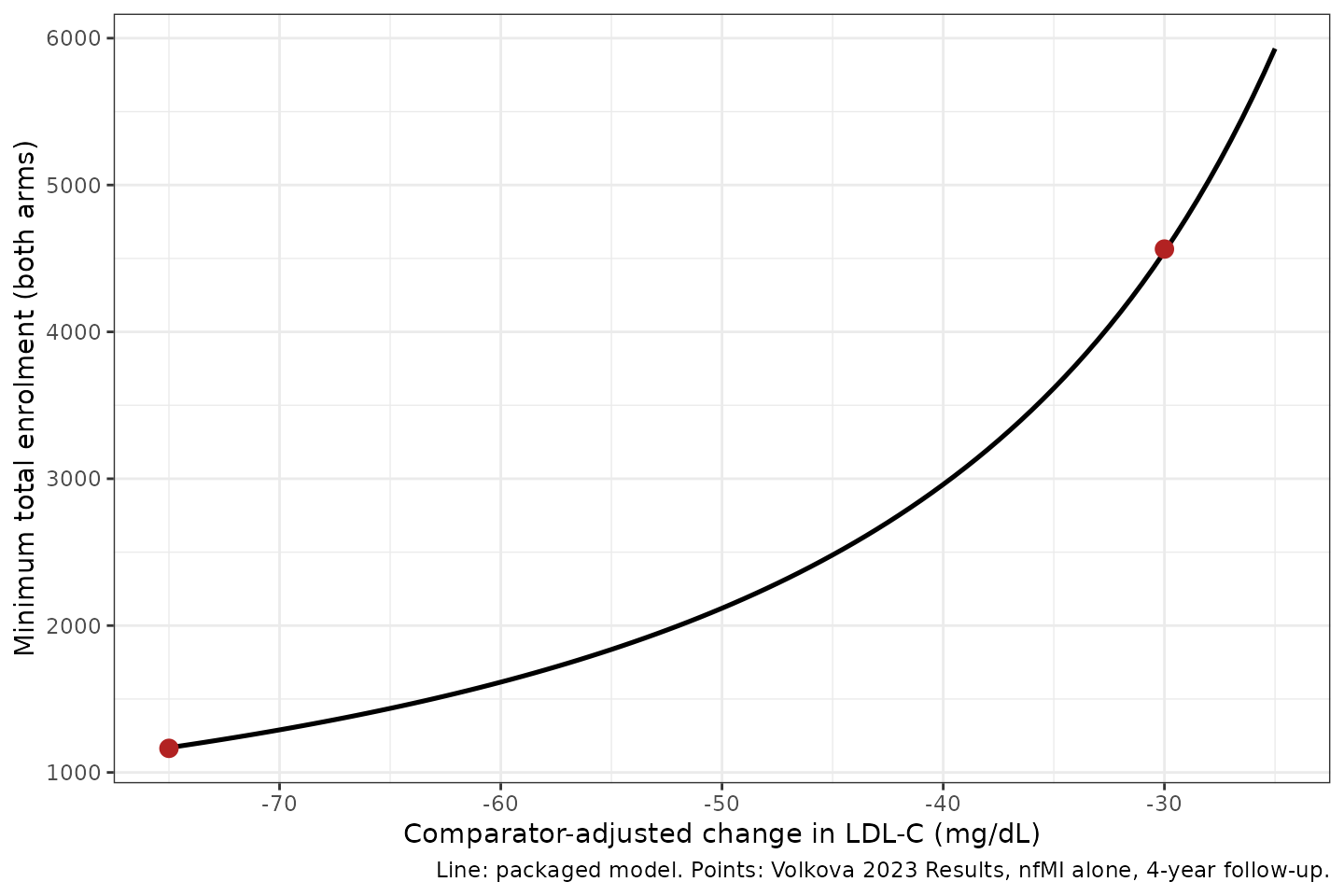
Volkova 2023 Figure 3, nonfatal-MI curve: minimum total enrolment required for a statistically significant risk reduction in a 4-year statin trial, versus comparator-adjusted LDL-C lowering. Points are the two sample sizes quoted in the paper’s Results.
fig3_chk <- solve_trials(make_trials(
  LDLC_DELTA   = c(-75, -30),
  LOGRR_TARGET = u_pts,
  K_CTRL       = k_nfmi
)) |>
  dplyr::transmute(
    dldlc = LDLC_DELTA,
    n_model = n_required,
    n_published = c(1164, 4564),
    pct_diff = 100 * (n_required - n_published) / n_published
  )

fig3_chk |>
  dplyr::rename("delta-LDL-C (mg/dL)" = dldlc, "Model N" = n_model,
                "Published N" = n_published, "Difference (%)" = pct_diff) |>
knitr::kable(digits = c(0, 0, 0, 2))| delta-LDL-C (mg/dL) | Model N | Published N | Difference (%) |
|---|---|---|---|
| -75 | 1169 | 1164 | 0.4 |
| -30 | 4546 | 4564 | -0.4 |
stopifnot(
  # Both published sample sizes are reproduced to better than 1% using a
  # single control-arm event rate. Deterministic algebra throughout, so a
  # tight bound is the correct assertion here.
  all(abs(fig3_chk$pct_diff) < 1)
)
The residual sub-1% spread is the signature of the paper’s uncertainty propagation: the published figures are medians over draws of the effect size and control-arm rate from their standard errors, whereas the formula evaluated at the point estimates is very slightly different. The agreement across a fourfold change in N confirms the two are the same calculation.
Composite MACE endpoints
Supplementary File 3 shows that a composite endpoint uses the same sample-size formula, with the effect size and control-arm rate replaced by the event-frequency-weighted aggregates. That is why the packaged model takes both as inputs rather than hard-coding one composition.
#' Aggregate component effect sizes and control-arm rates into the
#' composite equivalents (Volkova 2023 Supplementary File 3).
#'
#' Assumes, as the source does, that the number of patients experiencing
#' more than one component within a trial is negligible.
composite_inputs <- function(logrr, k) {
  list(
    logrr = log(sum(k * exp(logrr)) / sum(k)),
    k     = sum(k)
  )
}

# Sanity check: a "composite" of one event must return that event unchanged.
one <- composite_inputs(logrr = -0.657, k = k_nfmi)
stopifnot(
  abs(one$logrr - (-0.657)) < 1e-12,
  abs(one$k - k_nfmi) < 1e-12
)

# A worked two-component composite (nfMI + CR) at delta-LDL-C = -50 mg/dL.
# CR is the component Volkova 2023 identifies as most valuable to add to a
# 3-point MACE, because it is both frequent and strongly LDL-C-driven.
comp_pass1 <- solve_trials(make_trials(LDLC_DELTA = -50, TRT_PCSK9I = 0))

# Component control-arm rates: nfMI is the value recovered above; CR is
# NOT recoverable from any published number (see Errata), so it is varied
# across a plausible range rather than asserted.
k_cr_grid <- seq(0.02, 0.10, by = 0.005)

comp <- lapply(k_cr_grid, function(k_cr) {
  agg <- composite_inputs(
    logrr = c(comp_pass1$logrr_nfmi, comp_pass1$logrr_cr),
    k     = c(k_nfmi, k_cr)
  )
  data.frame(k_cr = k_cr, logrr_sum = agg$logrr, k_sum = agg$k)
}) |>
  dplyr::bind_rows()

# Derive k_cr back out of the solved K_CTRL rather than assuming rxSolve
# preserved the input row order, then sort explicitly -- the monotonicity
# assertion below is only meaningful on a sorted series.
comp_n <- solve_trials(make_trials(
  LOGRR_TARGET = comp$logrr_sum,
  K_CTRL       = comp$k_sum
)) |>
  dplyr::transmute(k_cr = K_CTRL - k_nfmi, n_composite = n_required) |>
  dplyr::arrange(k_cr)

# The single-endpoint nfMI comparator at the same delta-LDL-C.
n_nfmi_alone <- solve_trials(make_trials(
  LOGRR_TARGET = comp_pass1$logrr_nfmi, K_CTRL = k_nfmi
))$n_required

ggplot(comp_n, aes(x = k_cr, y = n_composite)) +
  geom_line(linewidth = 0.9) +
  geom_hline(yintercept = n_nfmi_alone, linetype = "dashed",
             colour = "firebrick") +
  scale_x_continuous(name = "Assumed 4-year control-arm CR event rate") +
  scale_y_continuous(name = "Minimum total enrolment (both arms)") +
  labs(caption = paste0(
    "Solid: nfMI + CR composite. Dashed: nfMI alone (N = ",
    round(n_nfmi_alone), "). delta-LDL-C = -50 mg/dL, statin, 4-year follow-up.")) +
  theme_bw()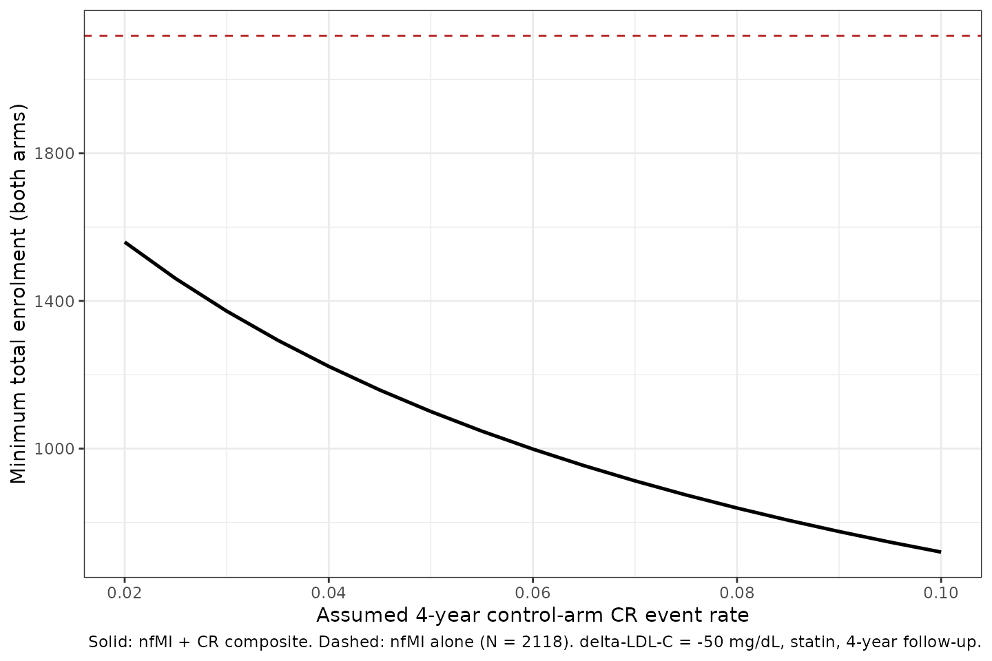
stopifnot(
  nrow(comp_n) == length(k_cr_grid), !anyNA(comp_n$n_composite),
  length(n_nfmi_alone) == 1L, is.finite(n_nfmi_alone),
  # The paper's headline mechanism: adding a frequent, strongly
  # LDL-C-driven component (CR) to nfMI always reduces the required
  # enrolment relative to nfMI alone, across the whole plausible range of
  # CR event rates. This is the quantitative form of "the most efficient
  # 4-point MACE ... was the combination of nfMI, nfST, CVM, and CR".
  all(comp_n$n_composite < n_nfmi_alone),
  # ... and the benefit grows as the added component becomes more frequent.
  all(diff(comp_n$n_composite) < 0)
)
This reproduces, on the endpoints this extraction carries, the paper’s central and slightly counter-intuitive conclusion: adding a component to a composite endpoint only increases power when that component is both frequent and carries a comparable effect size. Volkova 2023 found exactly this – coronary revascularization improved enrolment requirements substantially, whereas adding unstable angina or heart failure “did not provide significant benefit”.
Assumptions and deviations
Ten of fifteen endpoints. The five endpoints with therapy-only final models (fMI, hST, nfST, TIA, UA) are omitted because no numeric coefficient is published for them; they exist only as forest-plot points in Figure 2. This means the paper’s illustrative 3-point MACE (nfMI + nfST + CVM) cannot be reassembled here, since nfST is one of the five.
No between-trial variance. The meta-regressions are random-effects models, but tau-squared is not reported per endpoint. The model carries typical values only and predicts the meta-regression mean.
Control-arm event rates are user input.
K_CTRLis not computed from trial duration; the paper’s control-arm rate meta-regression is reported only graphically (Supplementary Figure 1). The nfMI value used in this vignette (about 0.043 at 4 years) was recovered by inverting the paper’s own published sample sizes at two independent points, not read off a figure. No value is available for any other endpoint, which is why the composite section varies the CR rate rather than asserting one.Covariates are entered uncentred, so several intercepts are extrapolations.
int_hf = +0.554is the predicted log(RR) at a baseline remnant cholesterol of 0 mg/dL, roughly 4 standard deviations below the lowest observed trial value. The intercepts are transcribed as published and are meaningful only in combination with a covariate value inside the observed range; supplying covariate values far outside the Supplementary Table 3 ranges will extrapolate.The Prevention indicators must be mutually exclusive. Exactly one of
PREVENT_PRIMARY,PREVENT_SECONDARY,PREVENT_MIXEDshould be 1. Setting more than one sums their age slopes, which the model does not guard against because rxode2 has no place to enforce it.RENALIMP_SEVis a trial-eligibility flag, not a patient stratum. It records whether the trial’s inclusion criteria admitted patients with severe renal disease, which is how Volkova 2023 coded it. The paper does not state the eGFR or creatinine-clearance threshold used.New canonical covariate names. This extraction registers
LDLC_DELTA,REMC,DIS_HYPERT_PERCENT,TRT_PCSK9I,PREVENT_PRIMARY,PREVENT_SECONDARY,PREVENT_MIXED,K_CTRLandLOGRR_TARGETininst/references/covariate-columns.md.unitsare placeholders. The model consumes no dose events and produces dimensionless risk ratios plus a subject count. Thedosingandconcentrationunit strings exist only to satisfy the dimensional-consistency check, following theYoshioka_2018_FXa_inhibitors_mbmaprecedent.