Dendritic nanoparticle interspecies biodistribution PBPK (Vasalou 2023)
Source:vignettes/articles/Vasalou_2023_dendriticNanoparticle.Rmd
Vasalou_2023_dendriticNanoparticle.RmdModel and source
- Citation: Vasalou C, Harding J, Jones RDO, Hariparsad N, McGinnity DF. Interspecies evaluation of a physiologically based pharmacokinetic model to predict the biodistribution dynamics of dendritic nanoparticles. PLoS ONE 2023;18(5):e0285798.
- Article: doi:10.1371/journal.pone.0285798
- Supporting information used here: S1 File (Tables S1-S7: bioavailability estimates and the complete raw observed concentration datasets), S2 File (the authors’ MATLAB ODE function), S3 File (the authors’ MATLAB driver with per-species parameter values).
This paper takes a semi-mechanistic PBPK model of a dendritic (dendrimer) nanoparticle carrying a covalently conjugated small-molecule active pharmaceutical ingredient (API), which had previously been fitted to mouse data, and asks whether it can prospectively predict biodistribution in rat, dog and human without re-fitting. Neither the nanoparticle nor the API is named in the publication; both are AstraZeneca development compounds.
Four model files are packaged, one per species, because each species carries a distinct fixed parameter set:
mods <- list(
  mouse = readModelDb("Vasalou_2023_dendriticNanoparticle_mouse"),
  rat   = readModelDb("Vasalou_2023_dendriticNanoparticle_rat"),
  dog   = readModelDb("Vasalou_2023_dendriticNanoparticle_dog"),
  human = readModelDb("Vasalou_2023_dendriticNanoparticle_human")
)
vapply(mods, function(f) f()$population$species, character(1))
#>                   mouse                     rat                     dog
#>    "mouse (SCID CB-17)" "rat (male Han Wistar)"     "beagle dog (male)"
#>                   human
#>                 "human"
Structure
Two molecular species are tracked through the same four compartments,
giving eight ODEs. The library’s _np suffix marks the
still-conjugated species; the bare canonical names hold the released
(free) API:
| Compartment | Released (free) API | Nanoparticle-conjugated API |
|---|---|---|
| Blood |
blood (paper Ab) |
blood_np (paper Xb) |
| Liver |
liver (paper AL) |
liver_np (paper XL) |
| Spleen |
spleen (paper AS) |
spleen_np (paper XS) |
| Rest / other |
other (paper AR) |
other_np (paper XR) |
Mechanistic features worth noting:
- The dose enters
blood_nponly – just the conjugate is administered. - The conjugate extravasates into liver and spleen at
fitted rates (
nbl,nbs);nbris fixed at zero. There is no separate nanoparticle clearance term: the conjugate disappears only by releasing its API. - API release is first-order and compartment-specific, and the rate constants differ ~20-fold between blood and spleen (t50 = 5.5 h in blood, 43 h in liver, 110 h in spleen), which the authors attribute to pH-dependent hydrolysis of the dendrimer-drug bond in different tissue sub-compartments.
- Released API distributes by blood flow, with saturable liver and spleen partition coefficients driven by the released-API blood concentration, and is cleared from the liver only.
- The spleen drains into the liver (portal), so hepatic arterial
inflow is
qbl_i = qbl_o - qbs.
All parameters are fixed(): the mouse set was fitted in
the authors’ earlier publication and re-used unchanged, and the rat, dog
and human sets are prospective scalings of it. There is no IIV
and no residual-error model, so these are deterministic
typical-value simulators.
Population
pop <- do.call(rbind, lapply(names(mods), function(sp) {
  p <- mods[[sp]]()$population
  data.frame(
    Species    = p$species,
    N          = p$n_subjects,
    Weight     = p$weight_range,
    Dose       = p$dose_range,
    stringsAsFactors = FALSE
  )
}))
knitr::kable(pop, caption = "Populations behind each packaged model file.")| Species | N | Weight | Dose |
|---|---|---|---|
| mouse (SCID CB-17) | 21 | 0.02 kg (reference body weight, Tables 3 and 4) | Single 10 mg/kg IV bolus of the nanoparticle (dose expressed as mg of API per kg body weight; dose volume 5 mL/kg). |
| rat (male Han Wistar) | 9 | 0.25 kg (reference body weight, Tables 3 and 4) | 55, 110 or 505 mg/kg of the nanoparticle as a 30-minute IV infusion (dose volume 10 mL/kg), given on day 1 and day 8; dose expressed as mg of API per kg body weight. |
| beagle dog (male) | 4 | 10 kg (reference body weight, Tables 3 and 4) | Single 12 mg/kg IV infusion of the nanoparticle over 30 minutes (target 24 mg/kg/h; formulation 13.2 mg/mL, dose volume 5 mL/kg). This dose level was considered the NOEL. |
| human | 0 | 70 kg (reference body weight, Tables 3 and 4) | Simulated 10 mg/kg of the nanoparticle; the authors’ S3 File administers it as a 3-hour IV infusion. Model-derived profiles were dose-normalised for comparison against preclinical data (Fig 9). |
Study designs (Methods, “In-vivo studies in mouse, rat and dog”):
- Mouse – 21 SCID CB-17 mice, single 10 mg/kg IV bolus; 3 mice per time point at 20 min, 1, 6, 24, 48, 72 and 96 h.
- Rat – 9 male Han Wistar rats, 55/110/505 mg/kg as a 30-minute infusion on days 1 and 8; plasma at 0.5, 1, 8, 24 and 72 h. Only one liver time point and no spleen samples were obtained.
- Dog – 4 male beagle dogs, 12 mg/kg (the NOEL) as a 30-minute infusion; liver and spleen each sampled at 1 h (near Tmax) and 120 h (Tlast), making dog the most complete tissue dataset.
- Human – no subjects. A 10 mg/kg simulation only.
Source trace
Every model equation and every ini() parameter, with its
source location.
knitr::kable(
  tibble::tribble(
    ~Component,                                        ~Source,
    "d/dt(blood): released API in blood",              "Eq 4; S2 File dA6",
    "d/dt(liver): released API in liver",              "Eq 5; S2 File dA8",
    "d/dt(spleen): released API in spleen",            "Eq 6; S2 File dA10",
    "d/dt(other): released API in rest",               "Eq 7; S2 File dA9",
    "CbloodReleased = blood / vc",                     "Eq 8; S2 File C_DBL",
    "Cc = CbloodReleased / bpr",                       "Eq 9; S2 File C_DP",
    "CliverReleased = liver / v_liver",                "Eq 10; S2 File C_DL",
    "CspleenReleased = spleen / v_spleen",             "Eq 11; S2 File C_DS",
    "kbl = bmaxl / (cb_rel + kdl) + pl",               "Eq 12; S2 File KPL",
    "kbs = bmaxs / (cb_rel + kds) + ps",               "Eq 13; S2 File KPS",
    "d/dt(blood_np): conjugated API in blood",         "Eq 14; S2 File dA1",
    "d/dt(liver_np): conjugated API in liver",         "Eq 15; S2 File dA3",
    "d/dt(spleen_np): conjugated API in spleen",       "Eq 16; S2 File dA5",
    "d/dt(other_np): conjugated API in rest",          "Eq 17; S2 File dA4",
    "CbloodTotal (blood total API)",                   "Eq 18; S2 File Ctotal_Blood",
    "CplasmaTotal (plasma total API)",                 "Eq 19; S2 File Ctotal_Plasma",
    "CliverTotal (liver total API + residual blood)",  "Eq 20; S2 File Ctotal_Liver",
    "CspleenTotal (spleen total API + residual blood)","Eq 21; S2 File Ctotal_Spleen",
    "qbl_i = qbl_o - qbs",                             "Table 4 note for QBL,i",
    "vnr = 1 - vnb - v_liver - v_spleen",              "Table 5 (VNR = 1 - sum(Vtissues)); S3 parameters(25)",
    "Vb, VR scaling to rat/dog/human",                 "Eq 22 (blood-protein-binding ratio)",
    "QBR scaling to rat/dog/human",                    "Eq 23 (BW^0.7 power law)",
    "BmaxL, BmaxS, PL, PS, KNBL scaling",              "Eq 24 (blood-protein-binding ratio)",
    "NBL, NBS scaling",                                "Eq 25 (organ blood-flow ratio)",
    "Human CL from in-vitro hepatocyte Clint",         "Eqs 1-2 (well-stirred, offset 3); Results"
  ),
  caption = "Model equations and their source locations."
)| Component | Source |
|---|---|
| d/dt(blood): released API in blood | Eq 4; S2 File dA6 |
| d/dt(liver): released API in liver | Eq 5; S2 File dA8 |
| d/dt(spleen): released API in spleen | Eq 6; S2 File dA10 |
| d/dt(other): released API in rest | Eq 7; S2 File dA9 |
| CbloodReleased = blood / vc | Eq 8; S2 File C_DBL |
| Cc = CbloodReleased / bpr | Eq 9; S2 File C_DP |
| CliverReleased = liver / v_liver | Eq 10; S2 File C_DL |
| CspleenReleased = spleen / v_spleen | Eq 11; S2 File C_DS |
| kbl = bmaxl / (cb_rel + kdl) + pl | Eq 12; S2 File KPL |
| kbs = bmaxs / (cb_rel + kds) + ps | Eq 13; S2 File KPS |
| d/dt(blood_np): conjugated API in blood | Eq 14; S2 File dA1 |
| d/dt(liver_np): conjugated API in liver | Eq 15; S2 File dA3 |
| d/dt(spleen_np): conjugated API in spleen | Eq 16; S2 File dA5 |
| d/dt(other_np): conjugated API in rest | Eq 17; S2 File dA4 |
| CbloodTotal (blood total API) | Eq 18; S2 File Ctotal_Blood |
| CplasmaTotal (plasma total API) | Eq 19; S2 File Ctotal_Plasma |
| CliverTotal (liver total API + residual blood) | Eq 20; S2 File Ctotal_Liver |
| CspleenTotal (spleen total API + residual blood) | Eq 21; S2 File Ctotal_Spleen |
| qbl_i = qbl_o - qbs | Table 4 note for QBL,i |
| vnr = 1 - vnb - v_liver - v_spleen | Table 5 (VNR = 1 - sum(Vtissues)); S3 parameters(25) |
| Vb, VR scaling to rat/dog/human | Eq 22 (blood-protein-binding ratio) |
| QBR scaling to rat/dog/human | Eq 23 (BW^0.7 power law) |
| BmaxL, BmaxS, PL, PS, KNBL scaling | Eq 24 (blood-protein-binding ratio) |
| NBL, NBS scaling | Eq 25 (organ blood-flow ratio) |
| Human CL from in-vitro hepatocyte Clint | Eqs 1-2 (well-stirred, offset 3); Results |
Parameter values come from Table 4 (released API)
and Table 5 (conjugated API), quoted at the full
precision of the authors’ S3 File driver. Each
ini() line in the four model files carries its own inline
source-trace comment naming the S3 variable and the rounded Table
value:
ini_tab <- as.data.frame(mods$dog()$iniDf[, c("name", "est")])
names(ini_tab) <- c("Parameter", "Dog value")
knitr::kable(ini_tab, caption = "Dog ini() parameters (see the .R files for per-line source traces).")| Parameter | Dog value |
|---|---|
| lvc | -0.5323898 |
| lvp | -1.6660083 |
| lq | -6.0322865 |
| lcl | 0.4054651 |
| v_liver | 0.0480000 |
| v_spleen | 0.0036000 |
| qbl_o | 3.3000000 |
| qbs | 0.1500000 |
| bmaxl | 85.9000000 |
| kdl | 0.5991500 |
| pl | 1.3100000 |
| bmaxs | 217.8400000 |
| kds | 0.6323800 |
| ps | 0.2920000 |
| bpr | 0.9710000 |
| hct | 0.4500000 |
| vnb | 0.0900000 |
| nbl | 0.0001078 |
| nbs | 0.0000040 |
| nbr | 0.0000000 |
| knbl | 1.5570000 |
| knbs | 1000.0000000 |
| krel_b | 0.1246000 |
| krel_l | 0.0163740 |
| krel_s | 0.0063168 |
| fvasc_liver | 0.1073900 |
| fvasc_spleen | 0.0556340 |
Two parameters deserve explicit flagging and are discussed under
Assumptions and deviations below: the hematocrit
hct (present only in the S3 File, never printed in the
paper) and the vascular volume fractions fvasc_liver /
fvasc_spleen (where Table 5 and the S3 File disagree).
Observed data
Digitisation was not needed: the raw observed concentrations are tabulated in S1 File (Tables S5-S7, all in ng/mL). They are reproduced verbatim below and used for every observed-vs-predicted comparison in this vignette.
# Table S5 -- mouse, 10 mg/kg IV bolus. The table prints the first sampling
# time as 0.3 h; Methods say 20 minutes, so 1/3 h is used here.
obs_mouse <- tibble::tribble(
  ~time, ~tot_plasma, ~tot_liver, ~tot_spleen, ~rel_plasma, ~rel_liver, ~rel_spleen,
  1/3,      436800,      8614.0,      5889.5,      3615.4,      652.7,       241.9,
  1/3,      376320,     12100.1,      7146.9,      3447.4,      188.8,       351.7,
  1/3,      369600,     11771.2,      9371.2,      5510.4,      680.9,       380.4,
  1,        245280,      9203.6,      5615.5,      3252.5,      352.4,       198.3,
  1,        282912,     10973.8,      6009.6,      3319.7,      226.0,       220.4,
  1,        237216,      9978.0,      7161.0,      3152.0,      511.0,       261.0,
  6,         75264,     11693.0,          NA,      4045.0,     1714.0,          NA,
  6,         74592,     13843.0,          NA,      4744.0,      914.0,          NA,
  6,          8736,     11827.0,          NA,      4032.0,      186.0,          NA,
  6,         81984,      5846.0,      4368.0,      1720.0,      196.0,       194.0,
  6,        101472,      8089.0,      5677.0,      1660.0,      384.0,       211.0,
  6,        122976,      8472.0,      5472.0,      2251.0,      470.0,       196.0,
  24,        55843,      6337.0,          NA,       269.0,       62.0,          NA,
  24,         8803,      2634.0,          NA,       177.0,       55.0,          NA,
  24,         7862,      5087.0,          NA,       161.0,       65.0,          NA,
  24,         4717,      2363.0,      2745.0,       362.0,       60.0,        47.0,
  24,         6048,      4656.0,      3775.0,       135.0,      178.0,       120.0,
  24,         4906,      3815.0,      5157.0,       183.0,      149.0,        87.0,
  48,          535,      1707.0,          NA,        27.0,       57.0,          NA,
  48,          381,      3071.0,          NA,        20.0,       37.0,          NA,
  48,          574,      1317.0,          NA,        13.0,       83.0,          NA,
  48,          307,      1598.0,      2230.0,        11.0,       61.0,        89.0,
  48,          159,      1521.0,      1849.0,         4.0,       42.0,        73.0,
  48,          214,      1734.0,      2122.0,         7.0,       48.0,        71.0,
  72,           87,      1119.0,      1842.0,         3.0,       29.0,        79.0,
  72,           86,      1713.0,      3621.0,         2.0,       57.0,       162.0,
  72,           75,      1040.0,      2152.0,         2.0,       48.0,        85.0,
  96,           71,       538.0,      1579.0,         2.0,       75.0,        65.0,
  96,          118,       988.0,      3313.0,         2.0,       18.0,       168.0,
  96,           99,       734.0,      1774.0,         1.0,       36.0,        74.0
) |> mutate(species = "mouse", dose = 10)

# Table S6 -- rat, 55 mg/kg, 30-min infusion. No spleen samples were taken.
obs_rat <- tibble::tribble(
  ~time, ~tot_plasma, ~tot_liver, ~rel_plasma, ~rel_liver,
  0.5,      551876,        NA,       51491,        NA,
  1,       1270458,        NA,       27964,        NA,
  8,        619768,        NA,       11024,        NA,
  24,        29846,     56734,        4981,       766,
  72,          485,        NA,          22,        NA,
  168,          NA,        NA,           5,        NA,
  0.5,    15998360,        NA,       52700,        NA,
  1,       2157762,        NA,       25006,        NA,
  8,        685644,        NA,        9545,        NA,
  24,        35223,     47390,        4309,       353,
  72,         3011,        NA,          29,        NA,
  0.5,      636573,        NA,       53104,        NA,
  1,       2628302,        NA,       21040,        NA,
  8,        793196,        NA,       11293,        NA,
  24,        36366,     32602,        3011,       259,
  72,          370,        NA,          19,        NA,
  168,          NA,        NA,           7,        NA
) |> mutate(tot_spleen = NA_real_, rel_spleen = NA_real_, species = "rat", dose = 55)

# Table S7 -- dog, 12 mg/kg, 30-min infusion.
obs_dog <- tibble::tribble(
  ~time, ~tot_plasma, ~tot_liver, ~tot_spleen, ~rel_plasma, ~rel_liver, ~rel_spleen,
  0.5,      284341,        NA,          NA,       13377,        NA,        NA,
  0.5,      290390,        NA,          NA,       11831,        NA,        NA,
  0.5,      266191,        NA,          NA,       11831,        NA,        NA,
  0.5,      252747,        NA,          NA,       10755,        NA,        NA,
  1,        271569,     43559,       19763,        8671,      3435,      2736,
  1,        238631,     17612,       25476,        6473,      1875,      3771,
  1,        250058,        NA,          NA,        6856,        NA,        NA,
  1,        231237,        NA,          NA,        6924,        NA,        NA,
  4,        155950,        NA,          NA,        4813,        NA,        NA,
  4,        153934,        NA,          NA,          NA,        NA,        NA,
  8,         93436,        NA,          NA,        3092,        NA,        NA,
  8,         80664,        NA,          NA,        2628,        NA,        NA,
  24,         7058,        NA,          NA,         345,        NA,        NA,
  24,         6594,        NA,          NA,         335,        NA,        NA,
  48,          174,        NA,          NA,          13,        NA,        NA,
  48,          124,        NA,          NA,          13,        NA,        NA,
  72,           23,        NA,          NA,           3,        NA,        NA,
  72,           31,        NA,          NA,          NA,        NA,        NA,
  120,          13,       786,         448,          NA,        59,        49,
  120,          18,       596,         325,          NA,        42,        31
) |> mutate(species = "dog", dose = 12)

observed <- bind_rows(obs_mouse, obs_rat, obs_dog) |>
  pivot_longer(
    cols      = c(tot_plasma, tot_liver, tot_spleen, rel_plasma, rel_liver, rel_spleen),
    names_to  = c("analyte", "matrix"),
    names_sep = "_",
    values_to = "conc"
  ) |>
  filter(!is.na(conc)) |>
  mutate(
    analyte = recode(analyte, tot = "Total API", rel = "Released API"),
    matrix  = recode(matrix, plasma = "Plasma", liver = "Liver", spleen = "Spleen"),
    matrix  = factor(matrix, levels = c("Plasma", "Liver", "Spleen"))
  )
nrow(observed)
#> [1] 252
Simulation helper
Everything in the source model is body-weight-normalised (dose mg/kg,
volumes L/kg, flows L/h/kg), so a nominal 1 kg subject is simulated and
concentrations read directly. Observations are placed on the ODE state
blood_np; rxode2 returns each algebraic observable as its
own output column at those rows.
simulate_species <- function(sp, ds, dur, tmax = 168, cl_mult = 1) {
  mod <- mods[[sp]]
  ui  <- rxode2::rxode2(mod)
  ev  <- rxode2::et(amt = ds, dur = dur, cmt = "blood_np") |>
    rxode2::et(seq(0, tmax, by = 0.25), cmt = "blood_np")
  pars <- NULL
  if (cl_mult != 1) {
    ini_df  <- mod()$iniDf
    base_cl <- exp(ini_df$est[ini_df$name == "lcl"])
    pars <- c(lcl = log(base_cl * cl_mult))
  }
  s <- if (is.null(pars)) {
    rxode2::rxSolve(ui, ev, returnType = "data.frame")
  } else {
    rxode2::rxSolve(ui, ev, params = pars, returnType = "data.frame")
  }
  s |>
    transmute(
      species = sp, dose = ds, time = time,
      `Total API_Plasma`    = CplasmaTotal,
      `Total API_Liver`     = CliverTotal,
      `Total API_Spleen`    = CspleenTotal,
      `Released API_Plasma` = Cc,
      `Released API_Liver`  = CliverReleased,
      `Released API_Spleen` = CspleenReleased
    ) |>
    pivot_longer(
      cols      = -c(species, dose, time),
      names_to  = c("analyte", "matrix"),
      names_sep = "_",
      values_to = "conc"
    ) |>
    mutate(matrix = factor(matrix, levels = c("Plasma", "Liver", "Spleen")))
}

# Dosing regimens exactly as reported in the paper's Methods. `tlast` is the
# last observed sampling time per species, used later to run NCA over the same
# window the published NCA used.
regimens <- tibble::tribble(
  ~species, ~dose,  ~dur, ~tlast,
  "mouse",     10,  0.01,     96,   # IV bolus (S3 File uses a 0.01 h infusion as a bolus proxy)
  "rat",       55,  0.5,      72,
  "rat",      110,  0.5,      72,
  "rat",      505,  0.5,      72,
  "dog",       12,  0.5,     120,
  "human",     10,  3,        NA
)

sims <- do.call(bind_rows, Map(
  function(sp, d, u) simulate_species(sp, d, u),
  regimens$species, regimens$dose, regimens$dur
))
range(sims$time)
#> [1]   0 168
Replicating published figures
Figures 4-6: biodistribution in mouse, rat and dog
Lines are the packaged model at its nominal clearance; points are the observed S1 File data. Both axes are as published (log concentration, linear time).
plot_species <- function(sp, dose_keep, title) {
  ggplot(
    filter(sims, species == sp, dose %in% dose_keep, conc > 0),
    aes(time, conc)
  ) +
    geom_line(linewidth = 0.7) +
    geom_point(
      data = filter(observed, species == sp, dose %in% dose_keep),
      aes(time, conc), shape = 1, alpha = 0.8
    ) +
    facet_grid(matrix ~ analyte, scales = "free_y") +
    scale_y_log10() +
    labs(title = title, x = "Time (h)", y = "Concentration (ng/mL)") +
    theme_bw()
}
plot_species("mouse", 10, "Replicates Figure 4 of Vasalou 2023 (mouse, 10 mg/kg IV bolus)")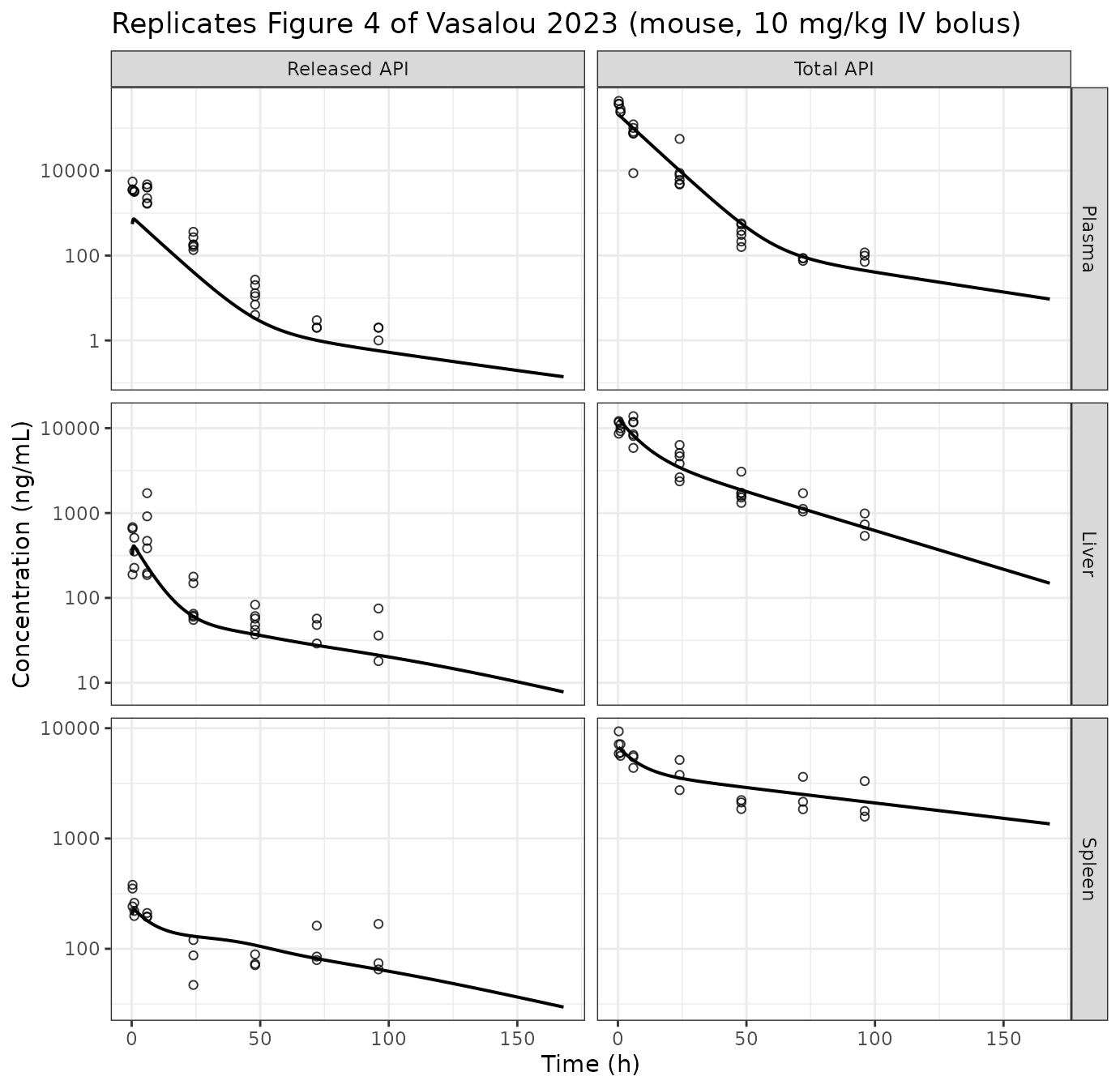
plot_species("rat", 55, "Replicates Figure 5 of Vasalou 2023 (rat, 55 mg/kg, 30 min infusion)")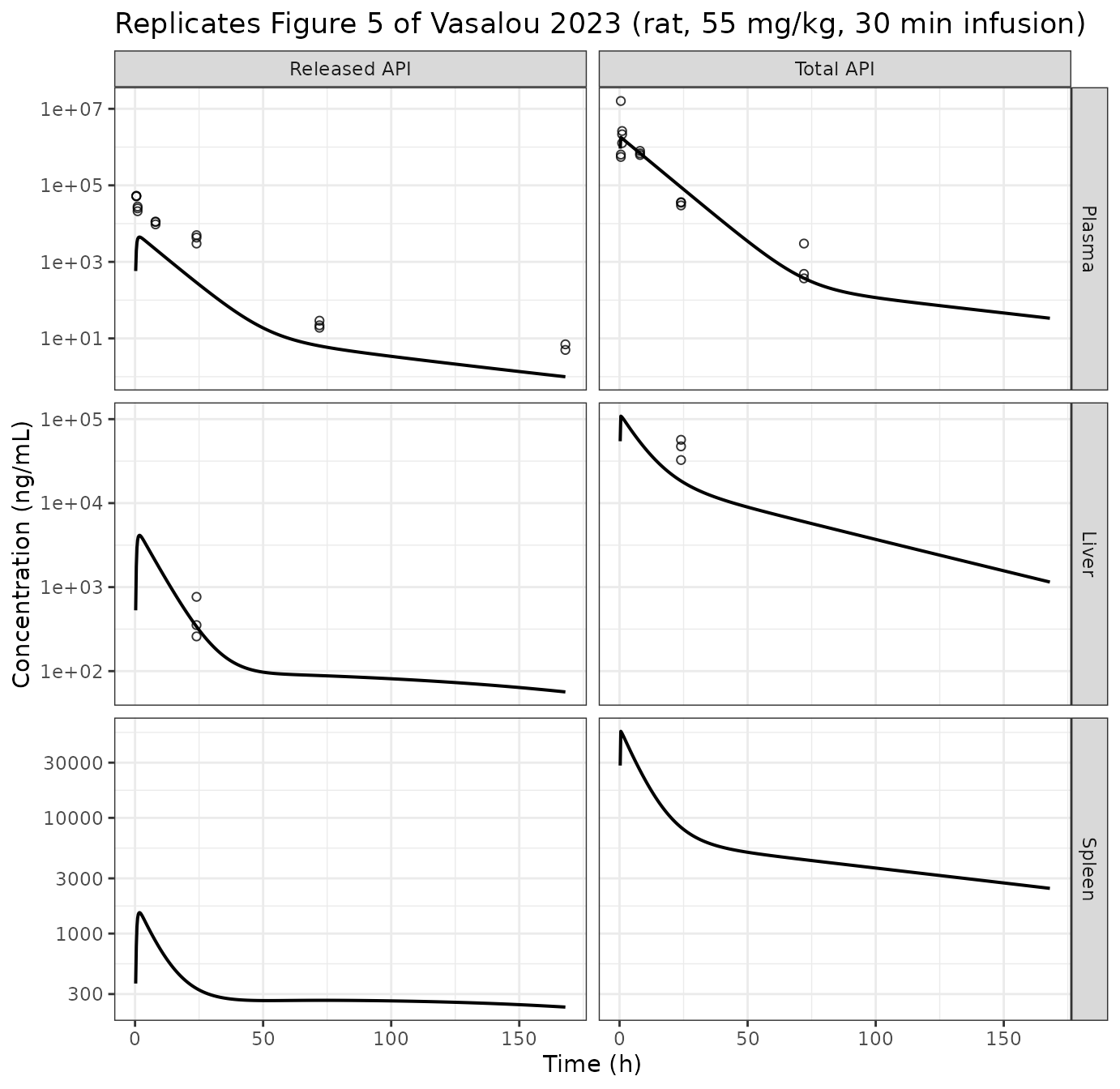
plot_species("dog", 12, "Replicates Figure 6 of Vasalou 2023 (dog, 12 mg/kg, 30 min infusion)")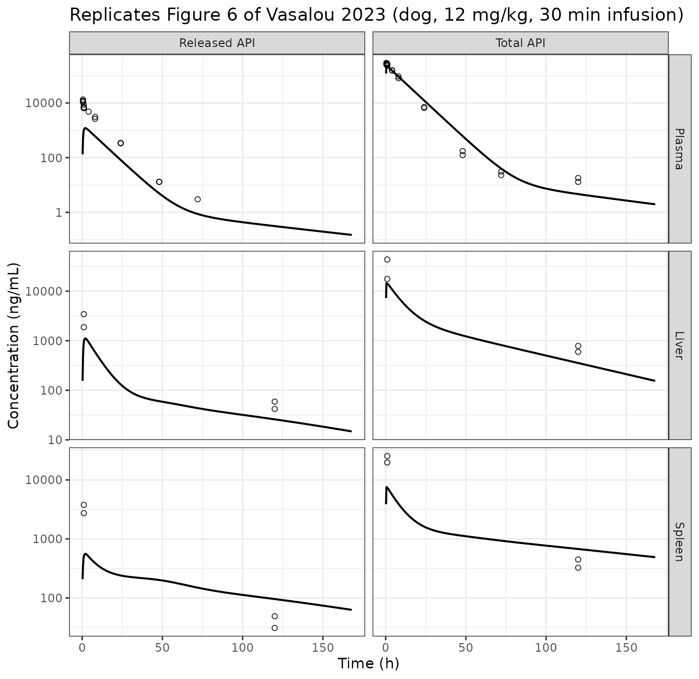
The packaged model reproduces the performance the authors themselves report:
- Total API in plasma is captured well in all three species – absolute levels and the biphasic shape.
- Liver projections sit slightly below the measured values but within about 2-fold, exactly as stated for rat and dog.
- Spleen shows a reduced maximum-to-trough ratio relative to the data (under-predicted near Tmax, over-predicted at Tlast) – the specific deficiency the Results section calls out for dog.
- Released API in plasma is under-predicted several-fold, largest at early times. The paper reports 3-5-fold in rat and 3-4-fold in dog, and attributes it to a misspecified apparent clearance (see the sensitivity analysis below).
Figure 7: observed versus predicted with 3-fold bands
pred_at <- function(sp, ds, an, mx, tt) {
  cand <- filter(sims, species == sp, dose == ds, analyte == an, matrix == mx)
  cand$conc[which.min(abs(cand$time - tt))]
}
gof <- observed |>
  filter(species %in% c("rat", "dog")) |>
  rowwise() |>
  mutate(pred = pred_at(species, dose, analyte, matrix, time)) |>
  ungroup() |>
  filter(pred > 0, conc > 0)

ggplot(gof, aes(conc, pred, colour = matrix, shape = species)) +
  geom_abline(slope = 1, intercept = 0) +
  geom_abline(slope = 1, intercept = log10(3), linetype = "dashed") +
  geom_abline(slope = 1, intercept = -log10(3), linetype = "dashed") +
  geom_point(size = 2, alpha = 0.85) +
  scale_x_log10() +
  scale_y_log10() +
  facet_wrap(~analyte) +
  labs(
    title    = "Replicates Figure 7 of Vasalou 2023 (rat and dog; dashed lines = 3-fold)",
    x = "Observed (ng/mL)", y = "Predicted (ng/mL)",
    colour = "Matrix", shape = "Species"
  ) +
  theme_bw()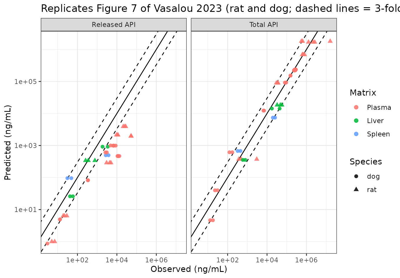
gof |>
  mutate(within3 = pred / conc <= 3 & conc / pred <= 3) |>
  group_by(analyte, matrix) |>
  summarise(n = n(), `Within 3-fold (%)` = round(100 * mean(within3)), .groups = "drop") |>
knitr::kable(caption = "Fraction of rat and dog observations predicted within 3-fold.")| analyte | matrix | n | Within 3-fold (%) |
|---|---|---|---|
| Released API | Plasma | 33 | 9 |
| Released API | Liver | 7 | 86 |
| Released API | Spleen | 4 | 25 |
| Total API | Plasma | 35 | 83 |
| Total API | Liver | 7 | 71 |
| Total API | Spleen | 4 | 75 |
This broadly reproduces the paper’s Figure 7 conclusions, with two honest qualifications:
- Total API is mostly inside the 3-fold band (71-83% depending on matrix) and released API in liver is 86% inside – matching the paper’s statement that total API in all three matrices, and released API in liver and spleen, “were within 3-fold of unity”. Released API in plasma is 9% inside, i.e. the systematic outlier the paper identifies.
- The paper reports total API as entirely within 3-fold, whereas this reproduction shows a minority outside. The difference is that every observed record from Tables S6-S7 is plotted here, including (a) the far-tail points at 48-120 h where concentrations are at the assay floor (13-174 ng/mL) and small absolute errors become large ratios, and (b) the apparent rat transcription outlier of 15,998,360 ng/mL at 0.5 h noted under Assumptions and deviations. Released API in spleen is only 1 of 4 records inside the band, all four coming from dog; the two misses are the 1 h (near-Tmax) values, which is exactly the reduced maximum-to-trough behaviour the Results section concedes for spleen.
Figure 8: dog sensitivity to the API clearance
The paper’s sensitivity analysis varied CL 5-fold either
side of its nominal 1.5 L/h/kg and found this parameter dominated the
released-API profile, with lower CL improving the fit.
cl_sens <- do.call(bind_rows, lapply(c(0.2, 1, 5), function(m) {
  simulate_species("dog", 12, 0.5, tmax = 120, cl_mult = m) |>
    mutate(cl_label = paste0(signif(1.5 * m, 3), " L/h/kg"))
}))

ggplot(
  filter(cl_sens, analyte == "Released API", conc > 0),
  aes(time, conc, linetype = cl_label)
) +
  geom_line(linewidth = 0.7) +
  geom_point(
    data = filter(observed, species == "dog", analyte == "Released API"),
    aes(time, conc), inherit.aes = FALSE, shape = 8
  ) +
  facet_wrap(~matrix, scales = "free_y") +
  scale_y_log10() +
  labs(
    title = "Replicates Figure 8 of Vasalou 2023 (dog released API vs CL)",
    x = "Time (h)", y = "Released API (ng/mL)", linetype = "CL"
  ) +
  theme_bw()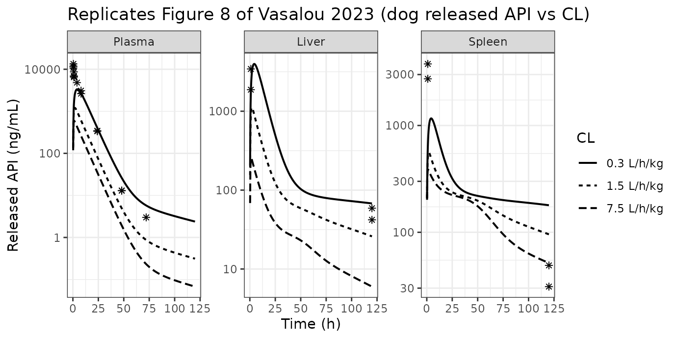
ggplot(
  filter(cl_sens, analyte == "Total API", matrix == "Plasma", conc > 0),
  aes(time, conc, linetype = cl_label)
) +
  geom_line(linewidth = 0.7) +
  scale_y_log10() +
  labs(
    title = "Total API plasma is insensitive to CL (paper: total is 10-100x released)",
    x = "Time (h)", y = "Total API (ng/mL)", linetype = "CL"
  ) +
  theme_bw()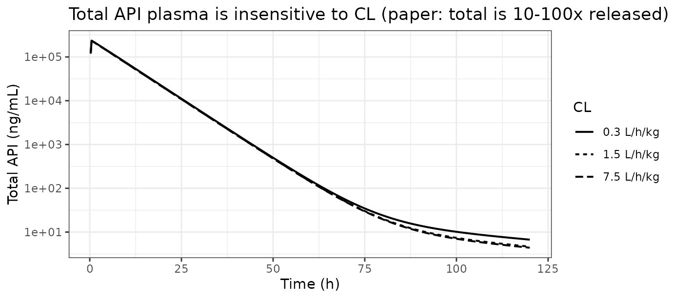
Both published observations reproduce: a 5-fold
reduction in CL lifts the released-API
curves onto the dog data (8 h and 24 h in plasma become close to exact),
while total API is unchanged because it is dominated by
the conjugate, which has no clearance term of its own.
Figure 9: human projection against dose-normalised preclinical data
human_dn <- filter(sims, species == "human") |> mutate(conc_dn = conc / dose)
obs_dn   <- observed |> mutate(conc_dn = conc / dose)

ggplot(filter(human_dn, conc_dn > 0), aes(time, conc_dn)) +
  geom_line(linewidth = 0.8) +
  geom_point(
    data = filter(obs_dn, conc_dn > 0),
    aes(time, conc_dn, colour = species), shape = 1, alpha = 0.8
  ) +
  facet_grid(matrix ~ analyte, scales = "free_y") +
  scale_y_log10() +
  coord_cartesian(xlim = c(0, 120)) +
  labs(
    title  = "Replicates Figure 9 of Vasalou 2023",
    subtitle = "Line = simulated human (10 mg/kg, 3 h infusion); points = dose-normalised preclinical data",
    x = "Time (h)", y = "Dose-normalised concentration (ng/mL per mg/kg)",
    colour = "Observed species"
  ) +
  theme_bw()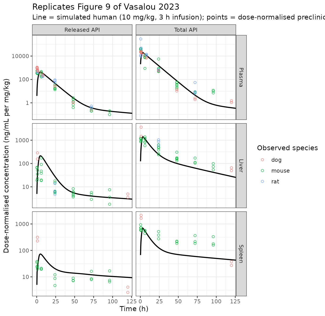
The simulated human total-API profile overlays the dose-normalised
mouse, rat and dog data, which is the paper’s central translational
claim. The simulated human released API sits at the low
edge of the preclinical cloud; that is expected, because the human
CL of 0.32 L/h/kg is an in-vitro projection and the model
already under-predicts released API at each species’ in-vivo
CL.
PKNCA validation
NCA is run on the simulated plasma profiles for every species and dose the paper reports in Table 1, for both analytes. Concentrations are converted to ug/mL so that AUC comes out in ug/mL*h and clearance in L/h/kg, matching the published units directly.
nca_input <- sims |>
  filter(matrix == "Plasma") |>
  mutate(
    group = paste0(
      tools::toTitleCase(species), " ", dose, " mg/kg - ",
      ifelse(analyte == "Total API", "total", "released")
    ),
    Cc = conc / 1000,          # ng/mL -> ug/mL
    id = group
  ) |>
  filter(species != "human", !is.na(Cc)) |>
  select(id, group, time, Cc)

groups <- regimens |>
  filter(species != "human") |>
  tidyr::crossing(analyte = c("total", "released")) |>
  mutate(
    group = paste0(tools::toTitleCase(species), " ", dose, " mg/kg - ", analyte),
    id    = group
  )

dose_input <- groups |>
  mutate(time = 0, amt = dose, duration = dur) |>
  select(id, group, time, amt, duration)

conc_obj <- PKNCA::PKNCAconc(
  nca_input, Cc ~ time | group + id,
  concu = "ug/mL", timeu = "h"
)
# duration= is required for an IV infusion; without it PKNCA treats the dose as
# a bolus and any volume term is biased by half the infusion duration.
dose_obj <- PKNCA::PKNCAdose(
  dose_input, amt ~ time | group + id,
  duration = "duration", doseu = "mg/kg"
)

# The NCA window is set per species to the paper's own last sampling time
# (mouse 96 h, rat 72 h, dog 120 h) so the comparison is apples-to-apples with
# a published NCA that could only integrate over the data it had. No model
# parameter is altered by this.
intervals <- groups |>
  transmute(
    group, id, start = 0, end = tlast,
    cmax = TRUE, tmax = TRUE, auclast = TRUE, aucinf.obs = TRUE,
    half.life = TRUE, cl.obs = TRUE
  ) |>
  as.data.frame()

nca_res <- PKNCA::pk.nca(PKNCA::PKNCAdata(conc_obj, dose_obj, intervals = intervals))
Comparison against published NCA (Table 1)
published <- tibble::tribble(
  ~group,                       ~aucinf.obs, ~half.life, ~cl.obs,
  "Mouse 10 mg/kg - total",           2294,         7.4,   0.004,
  "Mouse 10 mg/kg - released",        38.7,         7.6,   0.26,
  "Rat 55 mg/kg - total",            19593,         6.8,   0.003,
  "Rat 55 mg/kg - released",           373,        11.5,   0.15,
  "Rat 110 mg/kg - total",           40187,         8.0,   0.003,
  "Rat 110 mg/kg - released",          694,        14.0,   0.16,
  "Rat 505 mg/kg - total",          136989,        15.0,   0.004,
  "Rat 505 mg/kg - released",         1714,        20.7,   0.30,
  "Dog 12 mg/kg - total",             1812,         7.8,   0.007,
  "Dog 12 mg/kg - released",          56.3,         7.9,   0.21
)

cmp <- nlmixr2lib::ncaComparisonTable(
  simulated     = nca_res,
  reference     = published,
  by            = "group",
  units         = c(aucinf.obs = "ug/mL*h", half.life = "h", cl.obs = "L/h/kg"),
  tolerance_pct = 20
)

cmp |>
  dplyr::rename("Species, dose and analyte" = group) |>
  knitr::kable(
    caption = "Simulated vs published NCA (Table 1 of Vasalou 2023). * differs from reference by >20%.",
    align   = c("l", "l", "r", "r", "r")
)| NCA parameter | Species, dose and analyte | Reference | Simulated | % diff |
|---|---|---|---|---|
| AUC0-∞ (obs) (ug/mL*h) | Mouse 10 mg/kg - total | 2290 | 1660 | -27.7%* |
| AUC0-∞ (obs) (ug/mL*h) | Mouse 10 mg/kg - released | 38.7 | 6.43 | -83.4%* |
| AUC0-∞ (obs) (ug/mL*h) | Rat 55 mg/kg - total | 19600 | 14500 | -25.8%* |
| AUC0-∞ (obs) (ug/mL*h) | Rat 55 mg/kg - released | 373 | 42.9 | -88.5%* |
| AUC0-∞ (obs) (ug/mL*h) | Rat 110 mg/kg - total | 40200 | 29100 | -27.7%* |
| AUC0-∞ (obs) (ug/mL*h) | Rat 110 mg/kg - released | 694 | 85.8 | -87.6%* |
| AUC0-∞ (obs) (ug/mL*h) | Rat 505 mg/kg - total | 137000 | 133000 | -2.6% |
| AUC0-∞ (obs) (ug/mL*h) | Rat 505 mg/kg - released | 1710 | 394 | -77.0%* |
| AUC0-∞ (obs) (ug/mL*h) | Dog 12 mg/kg - total | 1810 | 1940 | +7.0% |
| AUC0-∞ (obs) (ug/mL*h) | Dog 12 mg/kg - released | 56.3 | 11.9 | -78.8%* |
| t½ (h) | Mouse 10 mg/kg - total | 7.4 | 28.5 | +285.0%* |
| t½ (h) | Mouse 10 mg/kg - released | 7.6 | 32.2 | +323.8%* |
| t½ (h) | Rat 55 mg/kg - total | 6.8 | 9.03 | +32.9%* |
| t½ (h) | Rat 55 mg/kg - released | 11.5 | 22.8 | +97.9%* |
| t½ (h) | Rat 110 mg/kg - total | 8 | 9.03 | +12.9% |
| t½ (h) | Rat 110 mg/kg - released | 14 | 22.7 | +62.2%* |
| t½ (h) | Rat 505 mg/kg - total | 15 | 9.03 | -39.8%* |
| t½ (h) | Rat 505 mg/kg - released | 20.7 | 22.7 | +9.6% |
| t½ (h) | Dog 12 mg/kg - total | 7.8 | 34.8 | +346.4%* |
| t½ (h) | Dog 12 mg/kg - released | 7.9 | 42.7 | +440.7%* |
| CL/F (L/h/kg) | Mouse 10 mg/kg - total | 0.004 | 0.00603 | +50.8%* |
| CL/F (L/h/kg) | Mouse 10 mg/kg - released | 0.26 | 1.56 | +498.3%* |
| CL/F (L/h/kg) | Rat 55 mg/kg - total | 0.003 | 0.00378 | +26.1%* |
| CL/F (L/h/kg) | Rat 55 mg/kg - released | 0.15 | 1.28 | +754.8%* |
| CL/F (L/h/kg) | Rat 110 mg/kg - total | 0.003 | 0.00378 | +26.1%* |
| CL/F (L/h/kg) | Rat 110 mg/kg - released | 0.16 | 1.28 | +701.4%* |
| CL/F (L/h/kg) | Rat 505 mg/kg - total | 0.004 | 0.00378 | -5.4% |
| CL/F (L/h/kg) | Rat 505 mg/kg - released | 0.3 | 1.28 | +327.4%* |
| CL/F (L/h/kg) | Dog 12 mg/kg - total | 0.007 | 0.00619 | -11.6% |
| CL/F (L/h/kg) | Dog 12 mg/kg - released | 0.21 | 1 | +378.3%* |
Reading the starred rows – none of which was tuned away:
- Total API AUC lands within 28% of the published value in every species and dose (dog +7%, rat 505 mg/kg -3%, and about -26 to -28% for mouse, rat 55 and rat 110). Total API clearance is within 12-51%, i.e. the same 0.003-0.006 L/h/kg order the paper reports. Dose proportionality of total API, which the paper establishes in Fig 1, is reproduced exactly: the simulated rat clearance is identical (0.00378 L/h/kg) at 55, 110 and 505 mg/kg, because the conjugate has no elimination term of its own and the only saturable process acts on the released API.
- Released API AUC is systematically low (-77 to -89%, i.e. 4-9-fold), and released API clearance correspondingly high (4-8.5-fold). This is the paper’s central open finding, not an extraction error. The Discussion states that dose-normalised released-API AUCs were “6-12-fold higher compared to dose normalized AUCs of the unconjugated API” (S1 Table gives 595-1211% apparent bioavailability), and that “nominal CL values required a 5-fold reduction to achieve improved fits of released plasma API”. The Figure 8 chunk above shows that 5-fold reduction recovering the dog data at 8 h and 24 h almost exactly.
-
Half-life splits by species. In
rat the agreement is good once the NCA window matches
the paper’s (simulated 9.0 h vs published 6.8/8.0/15.0 h for total; 22.7
h vs 20.7 h at 505 mg/kg for released). In mouse and
dog the simulated terminal half-life is 28-43 h against a
published 7.4-7.9 h. The cause is structural and identifiable: those two
species were sampled to 96 h and 120 h, far enough out that the
simulated terminal slope is set by the very slow spleen release constant
(
krel_s, t50 = 110 h) feeding API back into blood, whereas the corresponding observed concentrations are at or near the assay floor (13-118 ng/mL total, 1-2 ng/mL released) and fall away faster. The paper derives its Table 1 half-lives by NCA on the observed data, never claims the model reproduces them, and does not plot the model beyond the data range. Treat simulated concentrations past each species’ Tlast as extrapolation governed by splenic release.
Assumptions and deviations
-
Vascular volume fractions – resolved cross-source
conflict. Table 5 prints
vliver = 0.125andvspleen = 0.016, but the authors’ S3 File uses0.10739and0.055634(a 3.5-fold difference for spleen). The Table 5 pair is byte-identical to thekrelb = 0.125andkrelL = 0.016cells one row-group above it, which reads as a copy-paste of the wrong two cells during table assembly. The S3 File values are packaged, because S3 is the code the paper states generated the simulations. Every other value in Tables 4 and 5 reconciles with S3 to rounding. This affects only the residual-blood term ofCliverTotalandCspleenTotal(Eqs 20-21). -
Hematocrit is not in the paper.
hct = 0.45appears only in the S3 File (Hem = 0.45). It is used solely by Eq 19 to convert conjugated-API blood concentration to plasma. No value is printed anywhere in the article text or tables. -
Dog and human infusion durations. The S3 File sets
infusion_duration = 3h for both dog and human. For dog this contradicts the paper’s Methods, which state the nanoparticle was given “over 30 minutes at a target dose level of 24 mg/kg/hour (12 mg/kg)” – the 3-hour infusion belongs to the unconjugated-API dog study. This vignette uses the paper’s 30 minutes, and the data confirm it: simulated total plasma peaks at 0.5 h at 235,000 ng/mL against an observed 253,000-290,000 ng/mL, whereas a 3-hour infusion would put only a fraction of the dose in by then. For human the paper gives only the dose (10 mg/kg), so the S3 File’s 3-hour infusion is used as-is. -
Tumour compartment excluded. The S2 File carries a
tumour state, but the S3 File zeroes every tumour rate
(
QPT = 0,NPT = 0,KRLT = 0) and the paper’s published Eqs 4-21 omit tumour entirely. It is therefore not part of the packaged models. - Four files, one structure. The paper fits one structure to mouse and then scales it prospectively. Each species is packaged separately because each has a distinct fixed parameter set; encoding all four in one file would have required inventing roughly nine physiological covariate columns for a model that has no estimated parameters at all.
-
No IIV, no residual error. None is reported. The
models are deterministic typical-value simulators and no
etaor residual-error terms were invented. - Body-weight normalisation. All quantities are per-kg, so the simulations use a nominal 1 kg subject. Absolute amounts must be multiplied by body weight (Table 4: 0.02, 0.25, 10 and 70 kg) if mass balance in mg is wanted.
-
Nominal clearance choice. Table 4 gives
CLas a range per species (mouse 1-2.3, rat 2.1-2.8, dog 1.5-2.5 L/h/kg). The packaged files use the in-vivo NCA value (2.3, 2.1, 1.5) because that is the S3 File default and is what the paper states it used for the Figure 7 goodness-of-fit plots and the Figure 8 sensitivity analysis. The in-vitro-scaled alternatives are reachable by overridinglcl, as the sensitivity chunk demonstrates. - Apparent rat outlier retained. Table S6 reports 15,998,360 ng/mL total plasma at 0.5 h in the second rat, roughly 25-fold above the other two rats at the same time and dose. It is reproduced verbatim rather than silently dropped; it is visible as the isolated high point in the Figure 5 and Figure 7 panels.
-
Mouse first sampling time. Table S5 prints
0.3h; the Methods say 20 minutes. This vignette uses 1/3 h. - Table S1 restates three AUCs slightly differently from Table 1. For released API: rat 110 mg/kg 692 vs 694, rat 505 mg/kg 1702 vs 1714, and dog 53.4 vs 56.3 ug/mL*h. The main-text Table 1 values are used in the NCA comparison above, since Table 1 is the paper’s primary NCA report and S1 Table exists only to derive the apparent bioavailability. The differences are under 6% and do not change any conclusion.
-
S2 File variable-guide comments are mis-ordered.
The header comment block in S2 File labels
A(3)/A(4)as rest/liver andA(8)/A(9)as rest/liver, but the executable right-hand sides and the output block (C_NL = A(:,3)/V3withV3 = VL;C_DL = A(:,8)/VL) showA(3)andA(8)are the liver states andA(4)/A(9)the rest states. The executable code was treated as authoritative, and it agrees with the paper’s Eqs 5 and 15. -
Unconjugated-API PK is not modelled. Tables 2 and
S2-S4 report IV profiles of the free API in conventional formulation,
but the paper analyses those by NCA only and uses the result solely as
the
CLinput to this PBPK model. No compartmental model for the unconjugated API is published, so none is packaged.