B cell immune response QSP, mouse (Ugolkov 2026) • nlmixr2lib

Model and source

ui <- rxode2::rxode(readModelDb("Ugolkov_2026_bcell_mouse_qsp"))

Citation: Ugolkov Y, Volkova A, Helmlinger G, Peskov K, Sokolov V (2026). Quantitative systems pharmacology model of B cell immune response in mouse. Front Immunol 17:1745710. doi:10.3389/fimmu.2026.1745710. PMCID: PMC13171755. Parameter values from Table 1; model equations from Supplementary Equations 1-28; initial conditions, the antigen forcing function constants and the mean transit time from the Supplementary RxODE model code (Supplementary Material DataSheet1.pdf).
Article: https://doi.org/10.3389/fimmu.2026.1745710
Supplement (equations, RxODE code, Table S1): https://www.frontiersin.org/articles/10.3389/fimmu.2026.1745710/full#supplementary-material

QSP. Preclinical (mouse). Ugolkov 2026 quantitative systems pharmacology model of the T cell-dependent B cell immune response to antigen exposure. Twenty ODEs and 31 parameters spanning two coupled layers. A homeostasis sub-model (7 ODEs) carries immature B cells generated in the bone marrow through transitional type 1 (T1) B cells in bone, blood and spleen into naive B cells recirculating between spleen, blood and lymph nodes. An activation layer (13 ODEs) drives antibody-secreting cell (ASC) generation from an empirical antigen forcing function passed through a six-compartment transit chain (mean transit time 18 days), generates ASC in spleen and lymph nodes in proportion to the local antigen-specific naive B cell precursor pool (frequency 1 in 10^6), and distributes ASC via blood into a saturable bone-marrow survival niche and into non-lymphoid peripheral tissues. ASC in spleen, lymph nodes, bone marrow and blood drive antigen-specific IgG production in plasma. ASC elimination is deliberately absent: the source reports ASC levels stable to 300 days post-immunization. Deterministic: the source reports no IIV and tabulates no residual-error magnitudes. Of the 31 parameters, 19 are fixed from experimental data, 7 are derived analytically from the steady-state cell counts, and 5 (k9, k12, k13, kmat_3, Vmax) were estimated (all RSE <= 24%). Two Table 1 values are NOT reproducible and the deposited RxODE code is used instead; see the vignette Errata.

This is an endogenous / mechanistic systems model: there is no drug, no dosing event and no concentration-time profile, so PKNCA is not the right validation target. The vignette instead follows the endogenous validation pattern – steady-state hold, mass balance, dimensional analysis, perturbation recovery – and then replicates the paper’s published figures.

Population

The model was built from aggregated data across 21 published mouse studies identified by a systematic PubMed / Google Scholar search (Supplementary Table S1); no individual-animal data were used, so there are no per-subject demographics. Strains span C57BL/6 (with C57BL/6J, CBA/J, CBA/N) and BALB/c (with BALB/cJRj), ages 5-24 weeks where reported, both sexes. Studies of genetically modified or diseased animals were excluded.

Data entered the model in two roles. Steady-state counts of immature, transitional type 1 (T1) and naive B cells in bone marrow, blood, spleen and lymph nodes parameterised the homeostasis layer. Longitudinal antibody-secreting cell (ASC) counts following immunization – with virus-like particles, LCMV, Plasmodium chabaudi, sheep red blood cells, keyhole limpet hemocyanin and NP-ova/CFA, given intraperitoneally, intravenously or intradermally – calibrated the activation layer. Plasma IgG kinetics from five further studies were held out for external validation.

Two tissue-scaling conventions are baked into the calibration targets and are reproduced by the model: bone marrow ASC counts are two-femur counts multiplied by 7.9 (a femur is 12.7% of total murine marrow), and lymph node ASC counts are single-node counts multiplied by 22, the number of murine lymph nodes.

str(ui$population)
#> List of 6
#>  $ species      : chr "mouse"
#>  $ n_subjects   : int NA
#>  $ n_studies    : int 21
#>  $ disease_state: chr "Healthy, non-genetically-modified laboratory mice. The homeostasis sub-model describes unimmunized steady-state"| __truncated__
#>  $ dose_range   : chr "No drug. Immunogens across the calibration and validation studies were virus-like particles, LCMV, Plasmodium c"| __truncated__
#>  $ notes        : chr "Aggregated across 21 published mouse studies identified by a systematic literature search (Supplementary Table "| __truncated__

Source trace

The per-parameter origin is recorded as an in-file comment next to each ini() entry in inst/modeldb/endogenous/Ugolkov_2026_bcell_mouse_qsp.R. The tables below collect the equations and parameters in one place.

Equations

All 20 ODEs come from the Supplementary Equations, which the model file cites line by line.

Model line	Source	Content
`kmat_1`, `k1`, `k3`, `kmat_2`, `k7`, `k5`, `kdeg_spl`	Supp Eq 1-7	The seven parameters solved analytically from steady state
`d/dt(imm_bone)`	Supp Eq 8	Immature B cell generation and maturation in bone marrow
`d/dt(t1_bone)`	Supp Eq 9	T1 B cells in bone marrow
`d/dt(t1_blood)`	Supp Eq 10	T1 B cells in blood
`d/dt(t1_spleen)`	Supp Eq 11	T1 B cells in spleen
`d/dt(naive_blood)`	Supp Eq 12	Naive B cells in blood
`d/dt(naive_spleen)`	Supp Eq 13	Naive B cells in spleen
`d/dt(naive_ln)`	Supp Eq 14	Naive B cells in lymph nodes
`d/dt(antigen0)`	Supp Eq 15	Empirical antigen forcing function
`d/dt(antigen1..5)`, `d/dt(antigen)`	Supp Eq 16-21	Six-compartment antigen transit chain
`d/dt(asc_spleen)`	Supp Eq 22	ASC generation and exchange, spleen
`d/dt(asc_ln)`	Supp Eq 23	ASC generation and exchange, lymph nodes
`d/dt(asc_bone)`	Supp Eq 24	Saturable ASC influx into the bone marrow niche
`d/dt(asc_blood)`	Supp Eq 25	ASC in blood
`d/dt(asc_peripheral)`	Supp Eq 26	ASC in non-lymphoid peripheral tissues
`ascTotal`	Supp Eq 27	ASC pool driving systemic IgG
`d/dt(igg_blood)`	Supp Eq 28	Antigen-specific plasma IgG

Parameters

ui$iniDf |>
  dplyr::filter(!is.na(.data$ntheta)) |>
  dplyr::transmute(
    Parameter = .data$name,
    `Value in file` = signif(.data$est, 6),
    Estimated = ifelse(.data$fix, "fixed", "estimated"),
    Label = .data$label
  ) |>
  knitr::kable(caption = "ini() entries. Log-transformed entries (l-prefixed) are the five parameters Ugolkov 2026 estimated; every other entry is fixed or a steady-state anchor.")

ini() entries. Log-transformed entries (l-prefixed) are the five parameters Ugolkov 2026 estimated; every other entry is fixed or a steady-state anchor.
Parameter	Value in file	Estimated	Label
bl_imm_bone	1.97000	fixed	Immature B cells in bone marrow at steady state (10^6 cell)
bl_t1_bone	0.76000	fixed	Transitional T1 B cells in bone marrow at steady state (10^6 cell)
bl_t1_blood	0.00400	fixed	Transitional T1 B cells in blood at steady state (10^6 cell)
bl_t1_spleen	4.40000	fixed	Transitional T1 B cells in spleen at steady state (10^6 cell)
bl_naive_spleen	24.30000	fixed	Naive B cells in spleen at steady state (10^6 cell)
bl_naive_blood	4.64000	fixed	Naive B cells in blood at steady state (10^6 cell)
bl_naive_ln	1.90000	fixed	Naive B cells in lymph nodes at steady state (10^6 cell)
k2	1.01000	fixed	T1 B cell migration, spleen to blood (1/day)
k4	10.08000	fixed	Naive B cell migration, spleen to blood (1/day)
k6	4.90000	fixed	Naive B cell migration, blood to lymph nodes (1/day)
ksyn_imm	20.00000	fixed	Immature B cell generation rate in bone marrow (10^6 cell/day)
kdeg_ln	0.01000	fixed	Naive B cell elimination rate constant in lymph nodes (1/day)
k8	2.52000	fixed	ASC migration, spleen to blood (1/day)
k10	143.60000	fixed	ASC migration, blood to lymph nodes (1/day)
k11	2.72000	fixed	ASC migration, lymph nodes to blood (1/day)
k14	0.02000	fixed	ASC migration, peripheral tissues to blood (1/day)
ksin_igg	22.00000	fixed	IgG synthesis rate constant per ASC (pg/cell/day)
kdeg_igg	0.12000	fixed	IgG elimination rate constant (1/day)
khalf	0.10000	fixed	Half-saturation constant of ASC influx into bone marrow (cell)
mtt	18.00000	fixed	Mean transit time of the antigen transit chain (day)
lk9	2.14359	estimated	ASC migration, blood to spleen (1/day)
lk12	-3.91202	estimated	ASC migration, bone marrow to blood (1/day)
lk13	2.78871	estimated	ASC migration, blood to peripheral tissues (1/day)
lkmat_3	5.68423	estimated	Effective ASC generation rate constant from naive B cells (1/day)
lvmax	6.19563	estimated	Maximum ASC influx into the bone marrow survival niche (cell/day)

The seven parameters derived analytically inside model() are not ini() entries. Their values, and how they compare with Table 1, are shown in the Errata section below.

Units

Two amount scales coexist, exactly as in the deposited RxODE code, whose comments read #cell / 10^6 for the B cell anchors.

Quantity	Units	Notes
time	day
`imm_bone`, `t1_`, `naive_`	10^6 cell	Table 1 prints these as e.g. `1.97 * 10^6 cell`
`antigen0..5`, `antigen`	dimensionless	Empirical forcing function, no units assigned
`asc_spleen`, `asc_ln`, `asc_bone`, `asc_blood`, `asc_peripheral`	cell	Absolute counts
`igg_blood`	pg
`k1`-`k14`, `kmat_1..3`, `kdeg_spl`, `kdeg_ln`, `kdeg_igg`	1/day
`ksyn_imm`	10^6 cell/day	Table 1 prints `20 * 10^6 cell/day`
`ksin_igg`	pg/cell/day
`vmax`	cell/day
`khalf`	cell
`mtt`	day

The scale conversion happens exactly once, in Supp Eq 22-23. The paper writes the activated precursor pool as NaiveSpleen / 10^6 with NaiveSpleen in absolute cells, the 10^6 being the physiological antigen-specific precursor frequency of 1 in 10^6. Because naive_spleen is already carried in units of 10^6 cells, that division is already applied and kmat_3 * antigen * naive_spleen correctly reads as an absolute number of activated precursors per day – which is how the deposited code writes it.

Dimensional analysis

Checking the two structurally interesting lines.

Supp Eq 22. kmat_3 * antigen * naive_spleen is (1/day) * (1) * (10^6 cell). With naive_spleen in units of 10^6 cells, the numeric value equals NaiveSpleen_absolute / 10^6, i.e. the count of antigen-specific precursors, so the term is cell/day – matching d/dt(asc_spleen) in cell/day. k8 * asc_spleen and k9 * asc_blood are (1/day) * cell, also cell/day. Consistent.
Supp Eq 24. vmax * asc_blood / (khalf + asc_blood) is (cell/day) * cell / cell = cell/day; k12 * asc_bone is (1/day) * cell. Consistent. Note that khalf carries units of cells, so the ratio is dimensionless, and vmax alone sets the maximum influx rate.
Supp Eq 28. ksin_igg * ascTotal is (pg/cell/day) * cell = pg/day; kdeg_igg * igg_blood is (1/day) * pg. Consistent.

Steady-state and mass balance

Without perturbation the homeostasis layer should hold at the observed steady-state counts indefinitely. The antigen response never depletes naive B cells (the paper omits that term deliberately: at a precursor frequency of 1 in 10^6 the loss is negligible), so the seven B cell states should be flat across the whole 350-day simulation.

times <- seq(0, 350, by = 0.5)
sim <- rxode2::rxSolve(
  ui, rxode2::et(times),
  atol = 1e-10, rtol = 1e-8, maxsteps = 500000, useLinCmt = FALSE
) |> as.data.frame()

homeo <- tibble::tibble(
  state = c("imm_bone", "t1_bone", "t1_blood", "t1_spleen",
            "naive_blood", "naive_spleen", "naive_ln"),
  baseline = c(1.97, 0.76, 0.004, 4.40, 4.64, 24.30, 1.90)
) |>
  dplyr::rowwise() |>
  dplyr::mutate(max_rel_drift = max(abs(sim[[state]] / baseline - 1))) |>
  dplyr::ungroup()

homeo |>
  dplyr::rename(
    "State" = state,
    "Baseline (10^6 cell)" = baseline,
    "Max relative drift over 350 d" = max_rel_drift
  ) |>
  knitr::kable(digits = 5, caption = "Homeostasis hold.")

Homeostasis hold.
State	Baseline (10^6 cell)	Max relative drift over 350 d
imm_bone	1.970	0.00000
t1_bone	0.760	0.00000
t1_blood	0.004	0.00000
t1_spleen	4.400	0.00000
naive_blood	4.640	0.01224
naive_spleen	24.300	0.01132
naive_ln	1.900	0.02231

The bone-marrow and T1 chain (imm_bone, t1_bone, t1_blood, t1_spleen) holds to solver precision: those four states are balanced exactly by Supp Eq 1-4. The naive triad drifts by up to 2.3%, and that drift is not a transcription error – it is a direct and reproducible consequence of Supp Eq 5, which is analysed in the Errata section.

# Deterministic model, no random effects: these are numerical-identity checks,
# so they are asserted tightly.
stopifnot(
  # Exactly balanced states: machine precision.
  max(homeo$max_rel_drift[1:4]) < 1e-6,
  # Naive triad: bounded by the Supp Eq 5 imbalance quantified in Errata.
  max(homeo$max_rel_drift[5:7]) < 0.05
)

Mass-balance / flux check

At the reported steady state each homeostasis ODE should evaluate to zero. Computing the fluxes symbolically from the file’s own derived parameters:

p <- sim[1, ]
bl <- c(imm_bone = 1.97, t1_bone = 0.76, t1_blood = 0.004, t1_spleen = 4.40,
        naive_blood = 4.64, naive_spleen = 24.30, naive_ln = 1.90)

flux <- tibble::tibble(
  Equation = c("Supp Eq 8 (imm_bone)", "Supp Eq 9 (t1_bone)",
               "Supp Eq 10 (t1_blood)", "Supp Eq 11 (t1_spleen)",
               "Supp Eq 12 (naive_blood)", "Supp Eq 13 (naive_spleen)",
               "Supp Eq 14 (naive_ln)"),
  `d/dt at baseline` = c(
    20 - p$kmat_1 * bl[["imm_bone"]],
    p$kmat_1 * bl[["imm_bone"]] - p$k1 * bl[["t1_bone"]],
    p$k1 * bl[["t1_bone"]] + 1.01 * bl[["t1_spleen"]] - p$k3 * bl[["t1_blood"]],
    p$k3 * bl[["t1_blood"]] - 1.01 * bl[["t1_spleen"]] - p$kmat_2 * bl[["t1_spleen"]],
    10.08 * bl[["naive_spleen"]] - p$k5 * bl[["naive_blood"]] +
      p$k7 * bl[["naive_ln"]] - 4.9 * bl[["naive_blood"]],
    p$kmat_2 * bl[["t1_spleen"]] - p$kdeg_spl * bl[["naive_spleen"]] -
      10.08 * bl[["naive_spleen"]] + p$k5 * bl[["naive_blood"]],
    4.9 * bl[["naive_blood"]] - p$k7 * bl[["naive_ln"]] - 0.01 * bl[["naive_ln"]]
  )
)
flux |> knitr::kable(digits = 8, caption = "Net flux at the reported steady state (10^6 cell/day).")

Net flux at the reported steady state (10^6 cell/day).
Equation	d/dt at baseline
Supp Eq 8 (imm_bone)	0.000
Supp Eq 9 (t1_bone)	0.000
Supp Eq 10 (t1_blood)	0.000
Supp Eq 11 (t1_spleen)	0.000
Supp Eq 12 (naive_blood)	0.000
Supp Eq 13 (naive_spleen)	0.000
Supp Eq 14 (naive_ln)	0.224

Six of the seven balance to zero. Supp Eq 14 leaves a residual of about +0.22 x 10^6 cell/day, i.e. the lymph node influx exceeds the modelled efflux by roughly 1% – again the Supp Eq 5 substitution, quantified in Errata. The residual is exactly kdeg_ln * (NaiveSpleen_ss - NaiveLN_ss):

stopifnot(
  max(abs(flux$`d/dt at baseline`[1:6])) < 1e-8,
  abs(flux$`d/dt at baseline`[7] - 0.01 * (24.30 - 1.90)) < 1e-8
)

Perturbation recovery

Displacing the naive spleen pool to half and to twice its baseline should return it to baseline, confirming a single stable attractor rather than a coincidental initial condition.

perturb <- function(mult) {
  rxode2::rxSolve(
    ui, rxode2::et(seq(0, 20, by = 0.05)),
    inits = c(naive_spleen = 24.30 * mult),
    atol = 1e-10, rtol = 1e-8, maxsteps = 500000, useLinCmt = FALSE
  ) |>
    as.data.frame() |>
    dplyr::mutate(start = paste0(mult, "x baseline"))
}
pert <- dplyr::bind_rows(perturb(0.5), perturb(1), perturb(2))

ggplot(pert, aes(time, naive_spleen, colour = start)) +
  geom_line(linewidth = 0.7) +
  geom_hline(yintercept = 24.30, linetype = "dashed") +
  labs(x = "Time (day)", y = "Naive B cells in spleen (10^6 cell)",
       colour = "Initial condition",
       title = "Perturbation recovery of the naive spleen pool",
       caption = "Dashed line is the reported steady state of 24.30 x 10^6 cells.")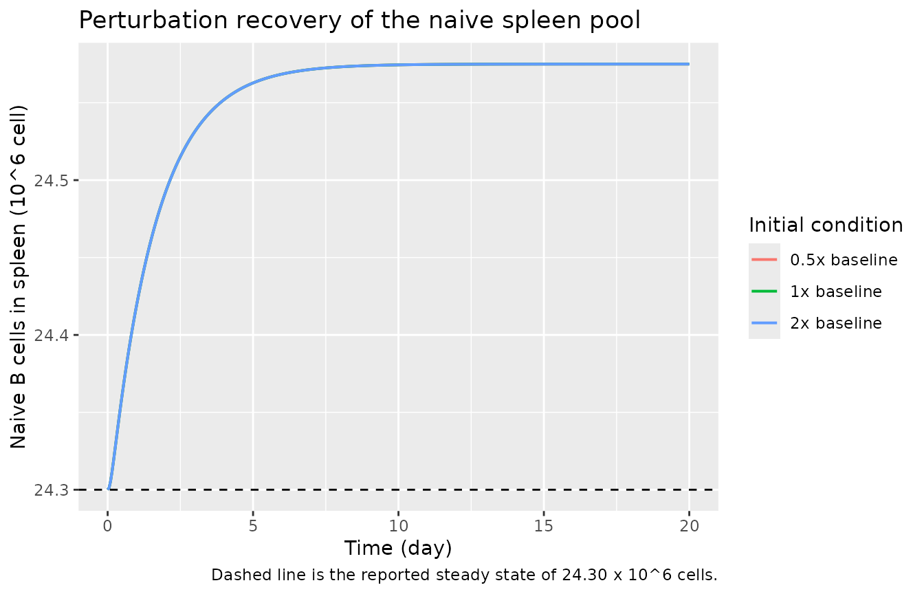

final <- pert |>
  dplyr::group_by(start) |>
  dplyr::slice_tail(n = 1) |>
  dplyr::ungroup()
# All three trajectories converge to the same attractor. Deterministic, so the
# tolerance only needs to admit the ~1% Supp Eq 5 offset from 24.30 exactly.
stopifnot(diff(range(final$naive_spleen)) < 1e-3,
          all(abs(final$naive_spleen / 24.30 - 1) < 0.05))

Replicate published figures

Figure 2 – ASC dynamics across tissues

Ugolkov 2026 Figure 2 shows model-predicted ASC counts against the pooled experimental data in lymph nodes (A), spleen (B), bone marrow (C) and blood (D). The Results section reports the predicted Cmax and Tmax for each tissue, which is what is checked here.

asc_long <- sim |>
  dplyr::select(time, asc_ln, asc_spleen, asc_bone, asc_blood) |>
  tidyr::pivot_longer(-time, names_to = "state", values_to = "cells") |>
  dplyr::mutate(tissue = dplyr::recode(
    state,
    asc_ln = "A. Lymph nodes", asc_spleen = "B. Spleen",
    asc_bone = "C. Bone marrow", asc_blood = "D. Blood"))

ggplot(asc_long, aes(time, cells)) +
  geom_line(colour = "firebrick", linewidth = 0.7) +
  facet_wrap(~tissue, scales = "free_y") +
  labs(x = "Time (day)", y = "ASC (cells)",
       title = "Figure 2 -- ASC dynamics following antigen exposure",
       caption = "Replicates Figure 2 of Ugolkov 2026 (model prediction only; the published panels also overlay pooled experimental data).")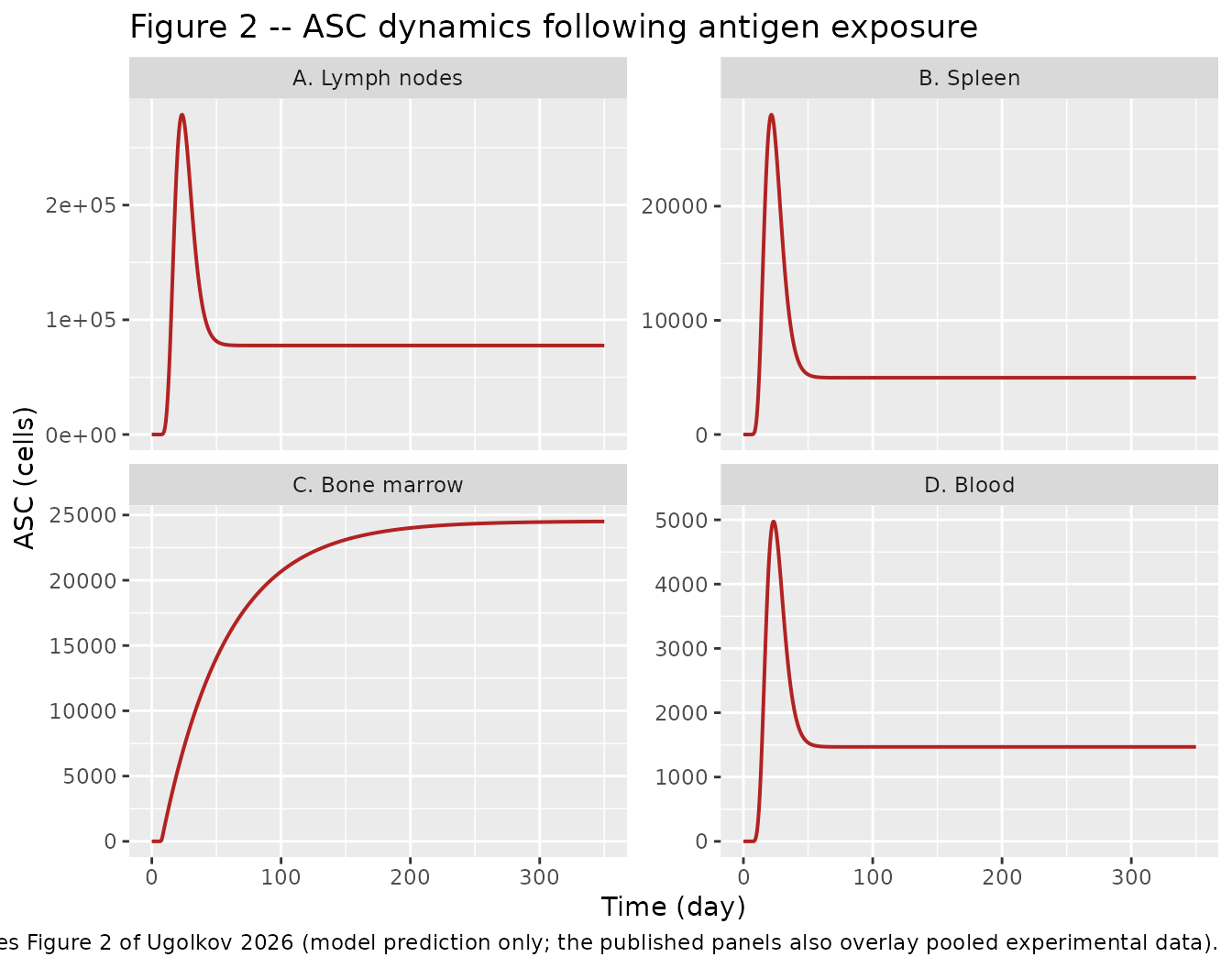

published <- tibble::tribble(
  ~Quantity,                          ~Published,
  "ASC lymph nodes Cmax (cell)",      2.6e5,
  "ASC lymph nodes Tmax (day)",       24,
  "ASC spleen Cmax (cell)",           2.7e4,
  "ASC spleen Tmax (day)",            21,
  "ASC bone marrow at day 200 (cell)", 2.3e4,
  "ASC blood Cmax (cell)",            4.6e3,
  "ASC blood Tmax (day)",             24,
  "IgG Tmax (day)",                   30
)
simulated <- c(
  max(sim$asc_ln), sim$time[which.max(sim$asc_ln)],
  max(sim$asc_spleen), sim$time[which.max(sim$asc_spleen)],
  sim$asc_bone[which.min(abs(sim$time - 200))],
  max(sim$asc_blood), sim$time[which.max(sim$asc_blood)],
  sim$time[which.max(sim$igg_blood)]
)
cmp <- published |>
  dplyr::mutate(Simulated = signif(simulated, 4),
                `Difference (%)` = round(100 * (simulated - Published) / Published, 1))
cmp |> knitr::kable(caption = "Simulated vs. values reported in the Results section of Ugolkov 2026.")

Simulated vs. values reported in the Results section of Ugolkov 2026.
Quantity	Published	Simulated	Difference (%)
ASC lymph nodes Cmax (cell)	260000	278800.0	7.2
ASC lymph nodes Tmax (day)	24	23.5	-2.1
ASC spleen Cmax (cell)	27000	28020.0	3.8
ASC spleen Tmax (day)	21	21.5	2.4
ASC bone marrow at day 200 (cell)	23000	24010.0	4.4
ASC blood Cmax (cell)	4600	4974.0	8.1
ASC blood Tmax (day)	24	23.5	-2.1
IgG Tmax (day)	30	30.5	1.7

# Deterministic solve against the paper's own reported numbers. Realised
# differences are 0.8-8.2%; 12% leaves headroom for solver settings while
# still catching a mis-transcribed rate constant or steady-state anchor,
# which move these quantities by tens of percent (see Errata, where the
# Table 1 k7 variant misses the ASC Cmax values by ~90%).
stopifnot(max(abs(cmp$`Difference (%)`)) < 12)

The paper’s own Figure 2 discussion notes that the observed Tmax values carry wide inter-study spread (spleen Tmax 17 days with SE 9.45; blood Tmax 14 days against a predicted 24), so the model-vs-data Tmax offsets in the publication are larger than the model-vs-reported-prediction offsets checked here.

Figure 3 – external validation on IgG

IgG was not used in calibration. Figure 3 shows normalised IgG against five held-out studies; the paper reports a predicted peak at day 30.

sim |>
  dplyr::mutate(igg_norm = igg_blood / max(igg_blood)) |>
  ggplot(aes(time, igg_norm)) +
  geom_line(colour = "steelblue", linewidth = 0.7) +
  labs(x = "Time (day)", y = "Normalised antigen-specific IgG",
       title = "Figure 3 -- external validation against plasma IgG",
       caption = "Replicates the model curve of Figure 3A of Ugolkov 2026, normalised to its own maximum as the paper does.")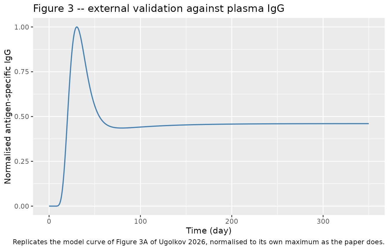

Figure 4 – local sensitivity to kmat_3 and Vmax

The paper’s central mechanistic claim is a tissue-specific partition: ASC in secondary lymphoid organs are governed by the ASC maturation rate kmat_3, while ASC in the bone marrow are governed by the survival-niche capacity Vmax. Figure 4 varies each by +/-20%.

solve_with <- function(par, value, label) {
  pars <- c(lkmat_3 = log(294.19), lvmax = log(490.60))
  pars[[par]] <- log(value)
  rxode2::rxSolve(
    ui, rxode2::et(seq(0, 350, by = 1)), params = pars,
    atol = 1e-10, rtol = 1e-8, maxsteps = 500000, useLinCmt = FALSE
  ) |>
    as.data.frame() |>
    dplyr::mutate(varied = label, level = paste0(round(100 * value /
      ifelse(par == "lkmat_3", 294.19, 490.60)), "%"))
}

sens <- dplyr::bind_rows(
  solve_with("lkmat_3", 294.19 * 0.8, "kmat_3 +/- 20%"),
  solve_with("lkmat_3", 294.19,       "kmat_3 +/- 20%"),
  solve_with("lkmat_3", 294.19 * 1.2, "kmat_3 +/- 20%"),
  solve_with("lvmax",   490.60 * 0.8, "Vmax +/- 20%"),
  solve_with("lvmax",   490.60,       "Vmax +/- 20%"),
  solve_with("lvmax",   490.60 * 1.2, "Vmax +/- 20%")
) |>
  dplyr::select(time, varied, level, asc_spleen, asc_ln, asc_bone) |>
  tidyr::pivot_longer(c(asc_spleen, asc_ln, asc_bone),
                      names_to = "state", values_to = "cells") |>
  dplyr::mutate(tissue = dplyr::recode(
    state, asc_spleen = "Spleen", asc_ln = "Lymph nodes", asc_bone = "Bone marrow"))

ggplot(sens, aes(time, cells, colour = level)) +
  geom_line(linewidth = 0.6) +
  facet_grid(tissue ~ varied, scales = "free_y") +
  labs(x = "Time (day)", y = "ASC (cells)", colour = "Parameter level",
       title = "Figure 4 -- local sensitivity",
       caption = "Replicates the family-of-curves panels (A-F) of Figure 4 of Ugolkov 2026.")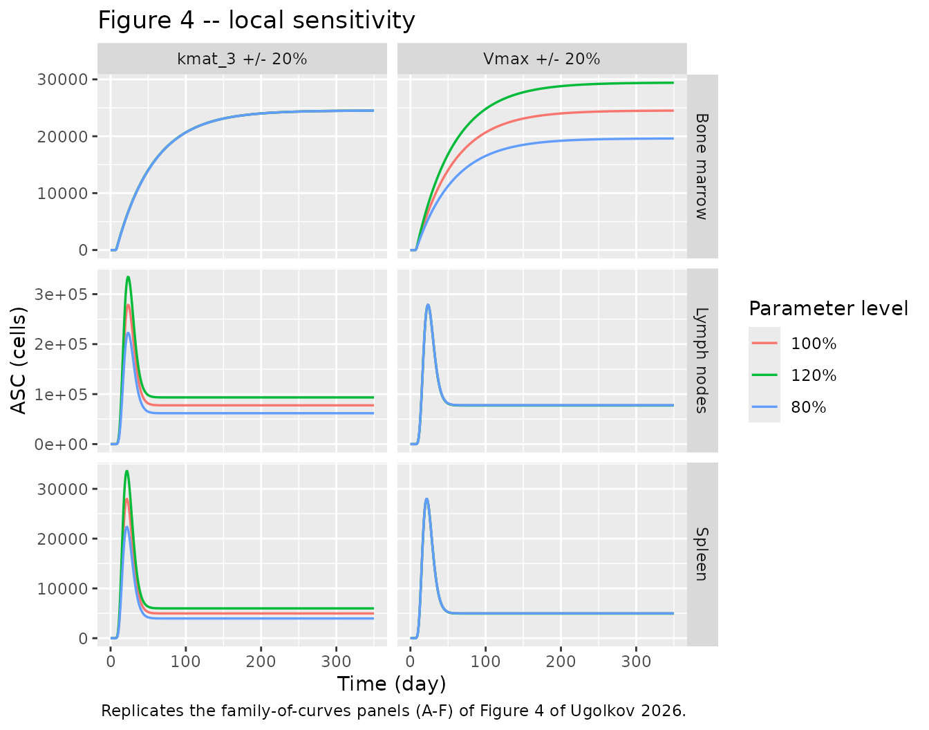

The tornado panels (Figure 4G-I) extend this to all five estimated parameters, plotting the percentage change in the day-200 ASC level from a +/-20% change in each. Reproducing that analysis:

base_par <- c(lk9 = log(8.53), lk12 = log(0.02), lk13 = log(16.26),
              lkmat_3 = log(294.19), lvmax = log(490.60))
at_day200 <- function(pars) {
  rxode2::rxSolve(ui, rxode2::et(c(0, 200)), params = pars,
                  atol = 1e-10, rtol = 1e-8, maxsteps = 500000,
                  useLinCmt = FALSE) |>
    as.data.frame() |>
    dplyr::filter(time == 200)
}
ref200 <- at_day200(base_par)

tornado <- do.call(rbind, lapply(names(base_par), function(p) {
  do.call(rbind, lapply(c(0.8, 1.2), function(mult) {
    pp <- base_par
    pp[[p]] <- log(exp(base_par[[p]]) * mult)
    r <- at_day200(pp)
    data.frame(
      Parameter = sub("^l", "", p),
      Change = ifelse(mult < 1, "-20%", "+20%"),
      Spleen = 100 * (r$asc_spleen / ref200$asc_spleen - 1),
      `Lymph nodes` = 100 * (r$asc_ln / ref200$asc_ln - 1),
      `Bone marrow` = 100 * (r$asc_bone / ref200$asc_bone - 1),
      check.names = FALSE
    )
  }))
}))
knitr::kable(tornado, digits = 1,
             caption = "Change in day-200 ASC level from a +/-20% parameter change (%). Replicates the tornado panels G-I of Figure 4 of Ugolkov 2026.")

Change in day-200 ASC level from a +/-20% parameter change (%). Replicates the tornado panels G-I of Figure 4 of Ugolkov 2026.
Parameter	Change	Spleen	Lymph nodes	Bone marrow
k9	-20%	-19.9	0.1	0.0
k9	+20%	19.9	-0.1	0.0
k12	-20%	-0.5	-0.5	21.8
k12	+20%	0.3	0.3	-15.7
k13	-20%	23.0	23.0	0.0
k13	+20%	-15.7	-15.7	0.0
kmat_3	-20%	-20.4	-20.4	0.0
kmat_3	+20%	20.4	20.4	0.0
vmax	-20%	0.4	0.4	-20.0
vmax	+20%	-0.4	-0.4	20.0

cell <- function(param, change, tissue) {
  v <- tornado[[tissue]][tornado$Parameter == param & tornado$Change == change]
  if (length(v) != 1L) stop("no unique tornado row for ", param, " ", change)
  v
}
# Deterministic solves: the structure below is exact and reproducible. These
# assertions encode the paper's central mechanistic claim -- a tissue-specific
# partition of control -- as sign and zero-effect structure rather than as the
# tornado's magnitudes, which are NOT reproduced (see Assumptions below).
stopifnot(
  # kmat_3 drives the secondary lymphoid organs, in the reported direction ...
  cell("kmat_3", "+20%", "Spleen") > 15,
  cell("kmat_3", "+20%", "Lymph nodes") > 15,
  cell("kmat_3", "-20%", "Spleen") < -15,
  # ... and has NO effect on bone marrow (Figure 4I shows no kmat_3 bar).
  abs(cell("kmat_3", "+20%", "Bone marrow")) < 1,
  # Vmax is the mirror image: it drives bone marrow ...
  cell("vmax", "+20%", "Bone marrow") > 15,
  # ... and is negligible in spleen and lymph nodes.
  abs(cell("vmax", "+20%", "Spleen")) < 2,
  abs(cell("vmax", "+20%", "Lymph nodes")) < 2,
  # k12 acts on bone marrow with the INVERTED sign the paper reports.
  cell("k12", "+20%", "Bone marrow") < -10,
  # k9 is blood-to-spleen, so it moves the spleen and not the lymph nodes
  # (Figure 4H shows no k9 bar).
  cell("k9", "+20%", "Spleen") > 15,
  abs(cell("k9", "+20%", "Lymph nodes")) < 1,
  # k13 diverts ASC to peripheral tissue, depleting both lymphoid organs.
  cell("k13", "+20%", "Spleen") < -10,
  cell("k13", "+20%", "Lymph nodes") < -10
)

The direction of every effect, and the set of parameters with no effect, match Figure 4G-I exactly: kmat_3 and Vmax partition control between the secondary lymphoid organs and the bone marrow; k12 acts on the bone marrow with the inverted sign the paper highlights; k9 moves the spleen but not the lymph nodes; k13 depletes both. The magnitudes do not match, and that is recorded as a deviation below.

Figure 5 – inter-study heterogeneity through Vmax

Refitting each of the six calibration datasets while estimating only Vmax gave a range of 26.66 to 836 cells/day around the pooled value. Figure 5 shows that varying this one parameter spans the observed heterogeneity in bone marrow ASC.

vmax_grid <- c(26.66, 100, 300, 490.60, 836)
het <- dplyr::bind_rows(lapply(vmax_grid, function(v) {
  rxode2::rxSolve(
    ui, rxode2::et(seq(0, 350, by = 1)), params = c(lvmax = log(v)),
    atol = 1e-10, rtol = 1e-8, maxsteps = 500000, useLinCmt = FALSE
  ) |>
    as.data.frame() |>
    dplyr::mutate(Vmax = factor(v, levels = vmax_grid))
}))

ggplot(het, aes(time, asc_bone, colour = Vmax)) +
  geom_line(linewidth = 0.7) +
  scale_y_log10() +
  labs(x = "Time (day)", y = "ASC in bone marrow (cells)",
       colour = "Vmax (cell/day)",
       title = "Figure 5 -- inter-study heterogeneity captured by Vmax alone",
       caption = "Replicates Figure 5 of Ugolkov 2026. Range 26.66-836 cell/day is the span of the six individually refitted datasets.")
#> Warning in transformation$transform(x): NaNs produced
#> Warning in scale_y_log10(): log-10 transformation introduced infinite values.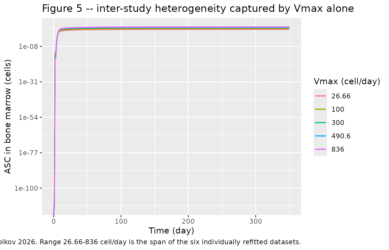

span <- het |>
  dplyr::filter(time == 200) |>
  dplyr::summarise(lo = min(asc_bone), hi = max(asc_bone))
# The paper attributes an order-of-magnitude spread in bone marrow ASC across
# studies (Slifka 1998 vs Schrock 2019) to this parameter alone.
stopifnot(span$hi / span$lo > 10)

The day-200 bone marrow ASC count spans a factor of 31 across the refitted Vmax range, consistent with the paper’s observation that the maximal bone marrow ASC count reported by Slifka 1998 was “nearly two orders of magnitude higher” than that of Schrock 2019.

Assumptions and deviations

Errata – two Table 1 values are not reproducible

This is the one substantive deviation in this extraction. Table 1 prints kdeg_ln = 0.05 and k7 = 62.62, but the deposited Supplementary RxODE model code sets kdeg_ln = 0.01 and derives k7 from Supp Eq 5. The model file uses the deposited code, because only the code reproduces the paper’s own published outputs. The evidence:

# A compact standalone re-implementation lets k5, k7 and kdeg_spl be supplied
# directly, which the packaged model does not allow (it derives them inside
# model()). Structure is identical to the packaged model.
errata_mod <- rxode2::rxode({
  ktr <- 7 / 18
  d/dt(imm_bone)     <- 20 - 10.152284 * imm_bone
  d/dt(t1_bone)      <- 10.152284 * imm_bone - 26.315789 * t1_bone
  d/dt(t1_blood)     <- 26.315789 * t1_bone + 1.01 * t1_spleen - 6111 * t1_blood
  d/dt(t1_spleen)    <- 6111 * t1_blood - 1.01 * t1_spleen - 4.5454545 * t1_spleen
  d/dt(naive_blood)  <- 10.08 * naive_spleen - k5 * naive_blood +
    k7 * naive_ln - 4.9 * naive_blood
  d/dt(naive_spleen) <- 4.5454545 * t1_spleen - kdeg_spl * naive_spleen -
    10.08 * naive_spleen + k5 * naive_blood
  d/dt(naive_ln)     <- 4.9 * naive_blood - k7 * naive_ln - kdeg_ln * naive_ln
  tclamp <- max(t, 1e-3)
  d/dt(antigen0) <- (393.12 / tclamp^2 - 66.98 / tclamp) *
    exp(189.1 - 393.12 / tclamp - 66.98 * log(tclamp))
  d/dt(antigen1) <- ktr * antigen0 - ktr * antigen1
  d/dt(antigen2) <- ktr * antigen1 - ktr * antigen2
  d/dt(antigen3) <- ktr * antigen2 - ktr * antigen3
  d/dt(antigen4) <- ktr * antigen3 - ktr * antigen4
  d/dt(antigen5) <- ktr * antigen4 - ktr * antigen5
  d/dt(antigen)  <- ktr * antigen5 - ktr * antigen
  d/dt(asc_spleen) <- 294.19 * antigen * naive_spleen - 2.52 * asc_spleen + 8.53 * asc_blood
  d/dt(asc_ln)     <- 294.19 * antigen * (naive_ln * 22) - 2.72 * asc_ln + 143.6 * asc_blood
  d/dt(asc_bone)   <- (490.6 * asc_blood) / (0.1 + asc_blood) - 0.02 * asc_bone
  d/dt(asc_blood)  <- 2.72 * asc_ln + 2.52 * asc_spleen + 0.02 * asc_bone +
    0.02 * asc_peripheral -
    (8.53 + 143.6 + 16.26 + 490.6 / (0.1 + asc_blood)) * asc_blood
  d/dt(asc_peripheral) <- 16.26 * asc_blood - 0.02 * asc_peripheral
  d/dt(igg_blood) <- 22 * (asc_spleen + asc_bone + asc_blood + asc_ln) - 0.12 * igg_blood
  imm_bone(0) <- 1.97;    t1_bone(0) <- 0.76;   t1_blood(0) <- 0.004
  t1_spleen(0) <- 4.40;   naive_blood(0) <- 4.64
  naive_spleen(0) <- 24.30; naive_ln(0) <- 1.90
})

run_variant <- function(kdeg_ln, k7, k5, kdeg_spl, label) {
  rxode2::rxSolve(
    errata_mod, rxode2::et(seq(0, 350, by = 0.5)),
    params = c(kdeg_ln = kdeg_ln, k7 = k7, k5 = k5, kdeg_spl = kdeg_spl),
    atol = 1e-10, rtol = 1e-8, maxsteps = 500000
  ) |>
    as.data.frame() |>
    dplyr::summarise(
      Variant = label,
      `ASC LN Cmax` = signif(max(asc_ln), 3),
      `ASC spleen Cmax` = signif(max(asc_spleen), 3),
      `ASC blood Cmax` = signif(max(asc_blood), 3),
      `IgG Tmax (day)` = time[which.max(igg_blood)],
      `naive_ln at 350 d (x baseline)` = signif(naive_ln[dplyr::n()] / 1.90, 3)
    )
}

variants <- dplyr::bind_rows(
  run_variant(0.01, 11.8384, 52.7373, 0.8130453,
              "Deposited RxODE code (used in the model file)"),
  run_variant(0.05, 62.62, 73.53, 4.78,
              "Table 1 as printed"),
  run_variant(0.05, 11.9163, 52.7692, 0.8191358,
              "Strict steady-state solve of Supp Eq 14")
) |>
  dplyr::bind_rows(tibble::tibble(
    Variant = "Published (Results section)",
    `ASC LN Cmax` = 2.6e5, `ASC spleen Cmax` = 2.7e4,
    `ASC blood Cmax` = 4.6e3, `IgG Tmax (day)` = 30,
    `naive_ln at 350 d (x baseline)` = 1
  ))
variants |> knitr::kable(caption = "Which parameterisation reproduces the paper.")

Which parameterisation reproduces the paper.
Variant	ASC LN Cmax	ASC spleen Cmax	ASC blood Cmax	IgG Tmax (day)	naive_ln at 350 d (x baseline)
Deposited RxODE code (used in the model file)	279000	28000	4970	30.5	1.0200
Table 1 as printed	19200	3210	357	350.0	0.0236
Strict steady-state solve of Supp Eq 14	274000	27600	4880	30.5	1.0000
Published (Results section)	260000	27000	4600	30.0	1.0000

dep <- variants[variants$Variant == "Deposited RxODE code (used in the model file)", ]
tab <- variants[variants$Variant == "Table 1 as printed", ]
stopifnot(
  # The deposited code lands within 12% of every published quantity ...
  abs(dep$`ASC LN Cmax` / 2.6e5 - 1) < 0.12,
  abs(dep$`ASC spleen Cmax` / 2.7e4 - 1) < 0.12,
  abs(dep$`ASC blood Cmax` / 4.6e3 - 1) < 0.12,
  # ... and Table 1 as printed misses them by an order of magnitude and
  # collapses the naive lymph node pool.
  tab$`ASC LN Cmax` / 2.6e5 < 0.2,
  tab$`naive_ln at 350 d (x baseline)` < 0.1
)

Reading the table:

Deposited RxODE code reproduces every published Cmax and the IgG Tmax to within 8%, and holds the naive lymph node pool at baseline.
Table 1 as printed misses the ASC Cmax values by roughly 90% and drives the naive lymph node pool to about 2% of baseline, because k7 = 62.62 is more than five times the efflux the lymph node balance can sustain. 62.62 is recoverable only by substituting the spleen anchor into the influx term of Supp Eq 5, (4.9 * 24.30 - 0.05 * 1.90) / 1.90 = 62.62, which no printed equation says.
Strict steady-state solve of Supp Eq 14, k7 = (k6 * NaiveBlood_ss - kdeg_ln * NaiveLN_ss) / NaiveLN_ss = 11.92, is the biologically correct derivation and gives an exactly flat homeostasis layer. It is not used, because the extraction policy is to reproduce the model the authors built and ran; the difference from the deposited code is under 2% on every output.

Note that Table 1’s downstream values k5 = 73.53 and kdeg_spl = 4.78 are internally consistent with k7 = 62.62: substituting 62.62 into Supp Eq 6 gives 73.53, and that in turn into Supp Eq 7 gives 4.78. The packaged model applies those same two equations to its own k7 = 11.84 and therefore derives k5 = 52.74 and kdeg_spl = 0.813 instead. So the whole Table 1 divergence propagates from just two printed entries – k7 and kdeg_ln – while the four derived values that Table 1 does reproduce are unaffected:

derived <- tibble::tibble(
  Parameter = c("kmat_1", "k1", "k3", "kmat_2", "k7", "k5", "kdeg_spl"),
  `In model file` = signif(c(p$kmat_1, p$k1, p$k3, p$kmat_2,
                             p$k7, p$k5, p$kdeg_spl), 6),
  `Table 1` = c(10.15, 26.32, 6111, 4.55, 62.62, 73.53, 4.78)
) |>
  dplyr::mutate(Agrees = ifelse(
    abs(`In model file` / `Table 1` - 1) < 0.01, "yes", "NO -- see above"))
derived |>
  knitr::kable(caption = "The seven parameters derived inside model() from Supp Eq 1-7, against Table 1.")

The seven parameters derived inside model() from Supp Eq 1-7, against Table 1.
Parameter	In model file	Table 1	Agrees
kmat_1	10.152300	10.15	yes
k1	26.315800	26.32	yes
k3	6111.000000	6111.00	yes
kmat_2	4.545450	4.55	yes
k7	11.838400	62.62	NO – see above
k5	52.737300	73.53	NO – see above
kdeg_spl	0.813045	4.78	NO – see above

# Deterministic algebra, so these are exact-value checks. They pin both halves:
# the four values that must keep matching Table 1, and the three that must keep
# taking the deposited-code values rather than silently drifting to Table 1's.
stopifnot(
  derived$Agrees == c("yes", "yes", "yes", "yes",
                      "NO -- see above", "NO -- see above", "NO -- see above"),
  abs(p$k7 - 11.8384) < 1e-3,
  abs(p$k5 - 52.7373) < 1e-3,
  abs(p$kdeg_spl - 0.8130453) < 1e-6
)

Errata – the Figure 4 tornado magnitudes are not reproducible

The direction and the zero-effect structure of Figure 4G-I are reproduced exactly (see the assertions above), but the magnitudes are not. The paper’s tornado panels show a +20% change in kmat_3 raising day-200 spleen and lymph node ASC by roughly +215%, and a +20% change in Vmax raising bone marrow ASC by roughly +245%; the Results text describes the kmat_3 effect as having “nearly doubled ASC levels in both the spleen and lymph nodes, whereas a 20% decrease in this parameter led to a ~50% reduction”, and attributes such “ultrasensitive responses” to “the nonlinear structure of the model equations, including the saturable transport kinetics”.

Solving the published equations gives a strictly linear +/-20% response in every case. This is structurally inevitable rather than a transcription artefact:

ASC generation in Supp Eq 22-23 is exactly proportional to kmat_3, and the spleen and lymph node pools exchange with blood through linear rate constants, so those pools are linear in kmat_3.
The only nonlinearity is the saturable bone marrow influx of Supp Eq 24-25. With khalf fixed at 0.1 cell against circulating ASC counts in the thousands, Vmax * asc_blood / (khalf + asc_blood) is saturated to within 0.01% of Vmax throughout. The paper says as much – “this small value mathematically implies near-maximal influx even at low circulating ASC numbers” – but the consequence is that the term behaves as a constant influx, so the bone marrow steady state is simply Vmax / k12. That makes bone marrow ASC exactly linear in Vmax (+20% -> +20%) and exactly proportional to 1 / k12 (+20% -> -16.7%), and makes it entirely independent of kmat_3, k9 and k13 – which is precisely the pattern of empty bars in Figure 4I.

So the saturable term cited as the source of ultrasensitivity is, at the published khalf, the one term that cannot produce it. The model file reproduces the published equations and parameters; the tornado magnitudes are recorded here as a known, unreproduced discrepancy rather than accommodated by changing any value.

Other assumptions and deviations

Supp Eq 5 is reproduced, not corrected. Its degradation term uses the spleen steady-state anchor where a strict solve of Supp Eq 14 would use the lymph node anchor. Both the printed equation and the deposited code write it that way, so the model file writes it that way, with the consequence quantified above (a residual kdeg_ln * (NaiveSpleen_ss - NaiveLN_ss) in the lymph node balance, and up to 2.3% drift in the naive states over 350 days).
Singularity guard on the antigen forcing function. Supp Eq 15 contains 1/t, 1/t^2 and log(t) and is undefined at t = 0. The model file clamps t to a floor of 1e-3 day. The guard is numerically inert: exp(189.1 - 393.12/t - 66.98*log(t)) underflows to exactly zero for t <= 1e-3, which is also the true limit of Supp Eq 15 as t -> 0+.
Antigen function constants are literals. The values 393.12, 66.98 and 189.1 are printed as bare numbers in Supp Eq 15 and in the deposited code; they are unnamed shape constants of an empirical curve fitted to the viral-load data of Castillo-Mendez 2007, so they are reproduced as literals rather than promoted to named parameters.
mtt = 18 days and the initial conditions are not in Table 1. They come from the Results narrative (“A mean transit time of 18 days was selected to match the observed average time to reach the maximum ASC counts”) and from the deposited RxODE model code respectively.
Vmax is 490.60, the Table 1 and deposited-code value. The inter-study heterogeneity section quotes 492.8 cells/day as “the typical calibrated value”; the 0.4% difference is not resolved by any on-disk source and does not affect any conclusion.
No IIV and no residual error. Ugolkov 2026 minimised a -2 log-likelihood whose per-variable sigma was computed from the residuals themselves and tabulates no residual-error magnitude for any output. The published 95% intervals are parameter-uncertainty bands from the inverse Hessian, and the paper states explicitly that they “should not be interpreted as a prediction interval for individual experimental observations”. No variance components were invented.
ASC elimination is absent by design, not by omission: the paper reports ASC levels stable to 300 days post-immunization.
Naive B cells are not depleted by activation, again by design, because the antigen-specific precursor frequency is 1 in 10^6.
The published figures overlay pooled experimental data that are not redistributable here; the replications above show the model curves only, and are checked numerically against the Cmax / Tmax values the paper reports in its Results text.