Frequency-domain response analysis of QSP models (Schulthess 2017)
Source:vignettes/articles/Schulthess_2017_frequency_domain_response_analysis.Rmd
Schulthess_2017_frequency_domain_response_analysis.Rmd
library(nlmixr2lib)
library(rxode2)
#> rxode2 5.1.8 using 2 threads (see ?getRxThreads)
#>   no cache: create with `rxCreateCache()`
library(dplyr)
#>
#> Attaching package: 'dplyr'
#> The following objects are masked from 'package:stats':
#>
#>     filter, lag
#> The following objects are masked from 'package:base':
#>
#>     intersect, setdiff, setequal, union
library(tidyr)
library(ggplot2)
Frequency-domain response analysis for quantitative systems pharmacology models (Schulthess 2017)
Schulthess, Post, Yates and van der Graaf (2018; published online
2017) introduce frequency-domain response analysis
(FdRA) to a pharmacometrics audience. FdRA is an engineering method:
instead of asking how a system responds over time, it asks how
the system transforms the harmonic content of its input. A
model is linearised around a stable steady state, written in state-space
form, and reduced to a transfer function
G(s) whose magnitude |G(i * 2 * pi * f)| is
exactly the ratio of output amplitude to input amplitude at frequency
f. Plotting that ratio against frequency gives a Bode plot,
and the shape of the Bode plot says which dosing frequencies a given PD
system amplifies and which it filters out.
The paper applies FdRA to 14 pharmacodynamic models drawn from four structural classes (indirect response, autoregulation, precursor-pool, and moderator-mediated feedback, the last in single- and double-moderator versions), plus a direct-effect model in the supplement that serves as the degenerate reference case. All 15 are shipped here as separate model files, because each is a genuinely different system of ODEs with its own frequency response. Every one is driven by the same one-compartment i.v. bolus PK model.
This is a tutorial: no data were fitted. Every
parameter is an illustrative constant printed in a figure caption, so
all of them are wrapped in fixed(), and none of the models
carries inter-individual variability or a residual-error model.
Population
There is no study population. The four PD structures are generic archetypes that the paper borrows from Gabrielsson and Hjorth (2016) to have something concrete to analyse:
| Class | Source case study | Biological setting |
|---|---|---|
| Indirect response | case study 3 | compound acting on the rat urinary bladder sphincter via a stimulatory alpha-2 adrenergic receptor; voiding volume as biomarker |
| Autoregulation | (generic) | auto-stimulatory or auto-inhibitory turnover with drug action on the loss |
| Precursor-pool | case study 16 | antilipolytic response of healthy volunteers to an adenosine receptor agonist |
| Moderator-mediated feedback | case study 18 | nicotinic acid inhibiting production of non-esterified free fatty acids |
| Double moderator-mediated feedback | case study 19 | fold mRNA induction of a target by an anonymised test compound |
Accordingly every model file records population$species
as
"not applicable (theoretical illustration; no subjects, no data fitted)"
with n_subjects = 0 and n_studies = 0.
Because there are no subjects, no doses of a real drug, and no measured concentrations, PKNCA is not an appropriate validation tool here and this vignette does not use it. Following the endogenous / mechanistic validation pattern, the model files are instead checked against (a) an exact steady-state hold, (b) an independently derived closed-form quasi-static limit, and (c) the published frequency-response characteristics of Table 1.
Source trace
Every equation and every ini() value, with its location
in the source.
| Quantity | Value | Source location |
|---|---|---|
Drug function E(c) = 1 +/- Emax * c / (EC50 + c)
|
– | Eq. 1 |
Indirect response ODE
dx/dt = kin * E(c) - kout * x
|
– | Eq. 2 (stimulation of production) |
Indirect response, loss flavors
dx/dt = kin - kout * x * E(c)
|
– | Figure 2a arrow position E3,4; ODE not printed (see
Errata) |
Indirect response steady state x_SS = kin / kout
|
1 | Eq. 3 |
One-compartment i.v. bolus PK dc/dt = -kel * c
|
– | Eq. 5 |
Autoregulation ODE
dx/dt = kin * phi(x) - kout * x * E(c)
|
– | Eq. 6 |
Feedback terms phi_1(x) = x/(K+x),
phi_2(x) = K/(K+x)
|
– | text following Eq. 6 |
Autoregulation steady state, positive feedback
kin/kout - K
|
0.75 | Analytical FdRA, autoregulation |
Autoregulation steady state, negative feedback
-K/2 + sqrt(K^2/4 + kin*K/kout)
|
0.390388 | Analytical FdRA, autoregulation |
Precursor-pool ODEs dx1/dt = kin - kout*x1*E(c),
dx2/dt = kout*x1*E(c) - kout*x2
|
– | Eq. 9 |
Precursor-pool steady state
x1_SS = x2_SS = kin/kout
|
1 | Analytical FdRA, precursor-pool |
Moderator ODEs dx1/dt = (kin/x2)*E(c) - kout*x1,
dx2/dt = ktol*(x1-x2)
|
– | Eq. 15 |
Moderator steady state
x1_SS = x2_SS = sqrt(kin/kout)
|
1 | Analytical FdRA, moderator-mediated feedback |
Double-moderator ODEs dx1/dt = (kin/x3)*E(c) - kout*x1,
dx2/dt = ktol*(x1-x2),
dx3/dt = ktol*(x2-x3)
|
– | Eq. 19 |
Double-moderator steady state sqrt(kin/kout)
|
1 | Analytical FdRA, double moderator |
Direct-effect model y = 1 +/- Emax*c/(EC50+c),
G(s) = +/- Emax/EC50
|
– | Supplementary text section A.2 |
kin |
1 mL/h | Figure 2, 3, 4, 5, 6 captions |
kout |
1 1/h | Figure 2, 3, 4, 5, 6 captions |
ktol |
0.25 1/h | Figure 5, 6 captions |
K (encoded as canonical kd) |
0.25 umol/L | Figure 3 caption |
Emax |
1 | Figure 2, 3, 4, 5, 6 and S1 captions |
EC50 |
0.25 umol/L | Figure 2, 3, 4, 5, 6 and S1 captions |
kel illustrative values |
1/24, 4 1/h (indirect, autoregulation, direct effect); 1/720, 1/6, 4 (precursor); 1/1440, 1/12, 4 (moderator, double moderator) | Figures 2d, 3d, 4d, 5d, 6d, S1a |
kel Bode sweep range |
10^-3 to 10^1 1/h | supplementary R script
(kes <- 10^seq(-3, 1, 0.1)) |
| Dose | 0.1 concentration units | supplementary R script (dose <- 0.1) |
| Dosing interval | 4 / kel |
Numerical FdRA text (“drug administration occurs at four times the inverse elimination rate”) |
| Amplitude measurement |
max - min over the tail of the simulation |
supplementary R script |
| Low-frequency gain read at |
kel = 2 * pi * 10^-5 1/h |
Table 1 footnote |
Load the models
modelIndex <- tibble::tribble(
  ~class,          ~flavor,             ~model,                                ~pd,
  "Indirect",      "Stim. production",  "Schulthess_2017_indirect_stim_kin",   "effect",
  "Indirect",      "Inhib. production", "Schulthess_2017_indirect_inhi_kin",   "effect",
  "Indirect",      "Stim. loss",        "Schulthess_2017_indirect_stim_kout",  "effect",
  "Indirect",      "Inhib. loss",       "Schulthess_2017_indirect_inhi_kout",  "effect",
  "Autoregulation", "Stim. + pos. fb",  "Schulthess_2017_autoreg_stim_posfb",  "effect",
  "Autoregulation", "Inhib. + pos. fb", "Schulthess_2017_autoreg_inhi_posfb",  "effect",
  "Autoregulation", "Stim. + neg. fb",  "Schulthess_2017_autoreg_stim_negfb",  "effect",
  "Autoregulation", "Inhib. + neg. fb", "Schulthess_2017_autoreg_inhi_negfb",  "effect",
  "Precursor-pool", "Stimulation",      "Schulthess_2017_precursor_stim",      "effect",
  "Precursor-pool", "Inhibition",       "Schulthess_2017_precursor_inhi",      "effect",
  "Moderator",     "Stimulation",       "Schulthess_2017_moderator_stim",      "effect",
  "Moderator",     "Inhibition",        "Schulthess_2017_moderator_inhi",      "effect",
  "Double moderator", "Stimulation",    "Schulthess_2017_moderator2_stim",     "effect",
  "Double moderator", "Inhibition",     "Schulthess_2017_moderator2_inhi",     "effect",
  "Direct effect",  "Stimulation",      "Schulthess_2017_directEffect_stim",   "directEffect"
)

models <- lapply(modelIndex$model, readModelDb)
names(models) <- modelIndex$model

readModelDb("Schulthess_2017_moderator_stim")
#> function() {
#>   description <- paste(
#>     "Theoretical (illustrative; no data fitted). Moderator-mediated feedback",
#>     "(tolerance) model with a STIMULATORY drug effect on the production of",
#>     "the response, driven by a one-compartment i.v. bolus PK model. Model",
#>     "flavor 1 of Figure 5a in Schulthess et al. (2017), used to demonstrate",
#>     "frequency-domain response analysis (FdRA). The response x1 stimulates a",
#>     "single endogenous moderator, which in turn divides the production rate",
#>     "of the response - a negative feedback loop that develops tolerance. The",
#>     "frequency response combines a low-pass and a band-pass: the linearised",
#>     "low-frequency gain is 2, the amplitude ratio peaks at 0.1 1/h, and the",
#>     "cutoff frequency is 0.04 1/h. The structure is case study 18 of",
#>     "Gabrielsson and Hjorth (2016) - nicotinic acid inhibiting the",
#>     "production of non-esterified free fatty acids (Isaksson et al. 2009).",
#>     sep = " "
#>   )
#>   reference <- paste(
#>     "Schulthess P, Post TM, Yates J, van der Graaf PH.",
#>     "Frequency-domain response analysis for quantitative systems",
#>     "pharmacology models.",
#>     "CPT Pharmacometrics Syst Pharmacol. 2018;7(2):111-123.",
#>     "doi:10.1002/psp4.12266.",
#>     sep = " "
#>   )
#>   vignette <- "Schulthess_2017_frequency_domain_response_analysis"
#>   units <- list(
#>     time = "h",
#>     dosing = "umol/L",
#>     concentration = "umol/L"
#>   )
#>
#>   # Issue #482: what each ODE state holds, in what amount units, in what
#>   # biological matrix. Verified against the source: the paper doses directly
#>   # in concentration units (Eq. 5 integrates the plasma concentration c
#>   # itself, and the supplementary R script adds dose = 0.1 to that state), so
#>   # the implied central volume is 1 and `central` carries a concentration.
#>   compartmentData <- list(
#>     central = list(analyte = "drug (generic)", units = "umol/L", specimen = "plasma", verified = TRUE),
#>     effect = list(
#>       analyte = "biomarker response x1 (the model output)",
#>       units = "mL",
#>       specimen = "plasma",
#>       verified = TRUE
#>     ),
#>     moderator1 = list(analyte = "endogenous moderator x2", units = "mL", specimen = "not applicable", verified = TRUE)
#>   )
#>
#>   population <- list(
#>     species = "not applicable (theoretical illustration; no subjects, no data fitted)",
#>     n_subjects = 0,
#>     n_studies = 0,
#>     disease_state = "not applicable (generic moderator-mediated turnover process)",
#>     dose_range = paste(
#>       "illustrative repeated i.v. bolus of 0.1 umol/L given every 4/kel h",
#>       "(supplementary R script); the Bode-plot analysis sweeps the",
#>       "elimination rate constant kel over 10^-3 to 10^1 1/h"
#>     ),
#>     notes = paste(
#>       "Schulthess et al. (2017) is a TUTORIAL introducing frequency-domain",
#>       "response analysis. No clinical or preclinical data were fitted, so",
#>       "there is no study population, no inter-individual variability and no",
#>       "residual-error model. Every parameter below is an illustrative",
#>       "constant printed in the Figure 5 caption and is therefore encoded",
#>       "with fixed(). The moderator is a Gabrielsson-Hjorth tolerance chain:",
#>       "a first-order delay driven by the response with NO mass transfer,",
#>       "whose value scales the production rate it modulates."
#>     )
#>   )
#>
#>   ini({
#>     # ---- One-compartment i.v. bolus PK (Eq. 5: dc/dt = -kel * c) ---------
#>     # The paper integrates the plasma CONCENTRATION directly and never
#>     # introduces a volume; the supplementary R script adds the dose to that
#>     # same state. vc is therefore fixed at 1 so that Cc == central, which
#>     # keeps the dimensional structure visible without changing any result.
#>     lvc  <- fixed(log(1))     ; label("Central volume of distribution Vc (L; implied = 1, see notes)")   # Eq. 5 - no volume in the source; dose is added directly to the concentration
#>     # kel is a SWEPT quantity, not an estimate. The value below is the
#>     # INTERMEDIATE elimination rate of the Figure 5d time course, the one
#>     # that shows the strongest amplification; the vignette sweeps kel over
#>     # 10^-3..10^1 1/h to build the Bode plot.
#>     lkel <- fixed(log(1 / 12)); label("Elimination rate constant kel (1/h)")                            # Figure 5d: elimination rates 1/1440, 1/12 and 4 1/h; 1/12 is the strongly amplifying case
#>
#>     # ---- Moderator-mediated turnover parameters -------------------------
#>     lkin  <- fixed(log(1))    ; label("Turnover rate of the response kin (mL/h)")                       # Figure 5 caption: kin = 1 mL/h
#>     lkout <- fixed(log(1))    ; label("Fractional turnover rate of the response kout (1/h)")            # Figure 5 caption: kout = 1 1/h
#>     lktol <- fixed(log(0.25)) ; label("Fractional turnover rate of the moderator ktol (1/h)")           # Figure 5 caption: ktol = 0.25 1/h
#>
#>     # ---- Drug function (Eq. 1: E(c) = 1 +/- Emax * c / (EC50 + c)) -------
#>     lemax <- fixed(log(1))    ; label("Maximum drug effect Emax (unitless)")                            # Figure 5 caption: Emax = 1
#>     lec50 <- fixed(log(0.25)) ; label("Concentration producing half-maximal effect EC50 (umol/L)")       # Figure 5 caption: EC50 = 0.25 umol/L
#>   })
#>
#>   model({
#>     vc   <- exp(lvc)
#>     kel  <- exp(lkel)
#>     kin  <- exp(lkin)
#>     kout <- exp(lkout)
#>     ktol <- exp(lktol)
#>     emax <- exp(lemax)
#>     ec50 <- exp(lec50)
#>
#>     # Unforced (c_SS = 0) stable steady state derived in the source:
#>     # x1_SS = x2_SS = sqrt(kin / kout). With the published values this is 1.
#>     effect(0)     <- sqrt(kin / kout)
#>     moderator1(0) <- sqrt(kin / kout)
#>
#>     d/dt(central) <- -kel * central
#>     Cc <- central / vc
#>
#>     # Eq. 1 with the stimulatory sign.
#>     drugEffect <- 1 + emax * Cc / (ec50 + Cc)
#>
#>     # Eq. 15 exactly:
#>     #   dx1/dt = (kin / x2) * E(c) - kout * x1
#>     #   dx2/dt = ktol * x1 - ktol * x2
#>     d/dt(effect)     <- (kin / moderator1) * drugEffect - kout * effect
#>     d/dt(moderator1) <- ktol * (effect - moderator1)
#>   })
#> }
#> <environment: 0x5581e2f3b0e0>
The published illustrative parameter set, shared by every model:
pars <- c(kin = 1, kout = 1, ktol = 0.25, kd = 0.25, emax = 1, ec50 = 0.25)
dose <- 0.1
pars
#>  kin kout ktol   kd emax ec50
#> 1.00 1.00 0.25 0.25 1.00 0.25
Check 1: the unforced steady state holds exactly
FdRA requires a stable steady state to linearise around, and
each model file sets its initial conditions to the steady state the
paper derives. With no dose given, every state must therefore stay
exactly where it started. This is a known-answer test of
kin, kout, ktol, kd
and of the algebraic form of each ODE simultaneously: get any one of
them wrong and the states drift.
ssExpected <- c(
  Schulthess_2017_indirect_stim_kin   = pars[["kin"]] / pars[["kout"]],
  Schulthess_2017_indirect_inhi_kin   = pars[["kin"]] / pars[["kout"]],
  Schulthess_2017_indirect_stim_kout  = pars[["kin"]] / pars[["kout"]],
  Schulthess_2017_indirect_inhi_kout  = pars[["kin"]] / pars[["kout"]],
  Schulthess_2017_autoreg_stim_posfb  = pars[["kin"]] / pars[["kout"]] - pars[["kd"]],
  Schulthess_2017_autoreg_inhi_posfb  = pars[["kin"]] / pars[["kout"]] - pars[["kd"]],
  Schulthess_2017_autoreg_stim_negfb  = -pars[["kd"]] / 2 +
    sqrt(pars[["kd"]]^2 / 4 + pars[["kin"]] * pars[["kd"]] / pars[["kout"]]),
  Schulthess_2017_autoreg_inhi_negfb  = -pars[["kd"]] / 2 +
    sqrt(pars[["kd"]]^2 / 4 + pars[["kin"]] * pars[["kd"]] / pars[["kout"]]),
  Schulthess_2017_precursor_stim      = pars[["kin"]] / pars[["kout"]],
  Schulthess_2017_precursor_inhi      = pars[["kin"]] / pars[["kout"]],
  Schulthess_2017_moderator_stim      = sqrt(pars[["kin"]] / pars[["kout"]]),
  Schulthess_2017_moderator_inhi      = sqrt(pars[["kin"]] / pars[["kout"]]),
  Schulthess_2017_moderator2_stim     = sqrt(pars[["kin"]] / pars[["kout"]]),
  Schulthess_2017_moderator2_inhi     = sqrt(pars[["kin"]] / pars[["kout"]])
)

ssCheck <- lapply(names(ssExpected), function(nm) {
  ev <- rxode2::et(seq(0, 500, by = 5), cmt = "central")
  s <- rxode2::rxSolve(models[[nm]], ev, atol = 1e-12, rtol = 1e-12,
                       returnType = "data.frame")
  tibble::tibble(
    model    = nm,
    expected = ssExpected[[nm]],
    drift    = max(abs(s$effect - ssExpected[[nm]]))
  )
}) |> bind_rows()

ssCheck |>
  rename("Model" = model, "Analytical steady state" = expected,
         "Max absolute drift over 500 h" = drift) |>
knitr::kable(digits = 10)| Model | Analytical steady state | Max absolute drift over 500 h |
|---|---|---|
| Schulthess_2017_indirect_stim_kin | 1.0000000 | 0 |
| Schulthess_2017_indirect_inhi_kin | 1.0000000 | 0 |
| Schulthess_2017_indirect_stim_kout | 1.0000000 | 0 |
| Schulthess_2017_indirect_inhi_kout | 1.0000000 | 0 |
| Schulthess_2017_autoreg_stim_posfb | 0.7500000 | 0 |
| Schulthess_2017_autoreg_inhi_posfb | 0.7500000 | 0 |
| Schulthess_2017_autoreg_stim_negfb | 0.3903882 | 0 |
| Schulthess_2017_autoreg_inhi_negfb | 0.3903882 | 0 |
| Schulthess_2017_precursor_stim | 1.0000000 | 0 |
| Schulthess_2017_precursor_inhi | 1.0000000 | 0 |
| Schulthess_2017_moderator_stim | 1.0000000 | 0 |
| Schulthess_2017_moderator_inhi | 1.0000000 | 0 |
| Schulthess_2017_moderator2_stim | 1.0000000 | 0 |
| Schulthess_2017_moderator2_inhi | 1.0000000 | 0 |
Every state is held to better than 1e-6 over 500 h, so all 14 ODE models sit on the steady state the paper derives.
Analytical FdRA: the closed-form transfer functions
The transfer function is
G(s) = Jyx (s I - Jxx)^-1 Jxc + Jyc, where Jxx
and Jxc are the Jacobians of the ODE system with respect to
the states and to the input, both evaluated at the unforced steady
state, and Jyx selects the output. For all 14 main-text
models Jyc = 0, which is exactly why they all filter the
input and why (as the paper’s Figure 7 notes) high-pass and band-stop
shapes cannot arise.
Working these out by hand for the published parameter set gives, with
b = kin * Emax / EC50 = 4:
-
Indirect response (all four flavors):
G(s) = b / (s + kout). The four flavors differ only in the sign and placement of the drug function, which linearisation discards, so their magnitudes coincide. -
Autoregulation:
G(s) = -kout * x_SS * (Emax/EC50) / (s - J)withJ = +/- kin*K/(K + x_SS)^2 - kout, the sign being positive for positive feedback and negative for negative feedback. -
Precursor-pool:
G(s) = b * s / (s + kout)^2. The factor ofsin the numerator forcesG(0) = 0: this is the band-pass. -
Moderator:
G(s) = b * (s + ktol) / ((s + kout)(s + ktol) + kout * ktol). -
Double moderator:
G(s) = b * (s + ktol)^2 / ((s + kout)(s + ktol)^2 + kout * ktol^2).
b <- pars[["kin"]] * pars[["emax"]] / pars[["ec50"]]

xssPos <- pars[["kin"]] / pars[["kout"]] - pars[["kd"]]
xssNeg <- -pars[["kd"]] / 2 +
  sqrt(pars[["kd"]]^2 / 4 + pars[["kin"]] * pars[["kd"]] / pars[["kout"]])

autoregG <- function(xss, feedbackSign) {
  jState <- feedbackSign * pars[["kin"]] * pars[["kd"]] / (pars[["kd"]] + xss)^2 -
    pars[["kout"]]
  jInput <- -pars[["kout"]] * xss * pars[["emax"]] / pars[["ec50"]]
  function(s) jInput / (s - jState)
}

transferFun <- list(
  Indirect           = function(s) b / (s + pars[["kout"]]),
  AutoregPos         = autoregG(xssPos, +1),
  AutoregNeg         = autoregG(xssNeg, -1),
  `Precursor-pool`   = function(s) b * s / (s + pars[["kout"]])^2,
  Moderator          = function(s) {
    b * (s + pars[["ktol"]]) /
      ((s + pars[["kout"]]) * (s + pars[["ktol"]]) + pars[["kout"]] * pars[["ktol"]])
  },
  `Double moderator` = function(s) {
    b * (s + pars[["ktol"]])^2 /
      ((s + pars[["kout"]]) * (s + pars[["ktol"]])^2 +
         pars[["kout"]] * pars[["ktol"]]^2)
  },
  `Direct effect`    = function(s) rep(b, length(s))
)
The paper’s five frequency-response characteristics, extracted from
each transfer function. Frequencies are
f = omega / (2 * pi), matching the supplementary R script,
which evaluates G at s = i * omega and plots
against omega / (2 * pi).
crossings <- function(fgrid, mag, level) {
  d <- mag - level
  idx <- which(d[-1] * d[-length(d)] < 0)
  if (!length(idx)) return(numeric(0))
  vapply(idx, function(i) {
    stats::approx(x = d[i:(i + 1)], y = fgrid[i:(i + 1)], xout = 0)$y
  }, numeric(1))
}

fdraChar <- function(G) {
  fgrid <- 10^seq(-6, 4, length.out = 400001)
  mag <- Mod(G(complex(imaginary = 2 * pi * fgrid)))
  g0 <- Mod(G(complex(real = 0, imaginary = 0)))
  ipk <- which.max(mag)
  cut <- if (g0 > 0) crossings(fgrid, mag, g0 / sqrt(2)) else numeric(0)
  thr <- crossings(fgrid, mag, 1)
  n <- length(fgrid)
  slope <- diff(log10(mag[c(n - 1000, n)])) / diff(log10(fgrid[c(n - 1000, n)]))
  list(
    lowFreqGain = g0,
    peakGain    = mag[ipk],
    peakFreq    = fgrid[ipk],
    cutoff      = if (length(cut)) max(cut) else NA_real_,
    threshold   = thr,
    relDegree   = -slope
  )
}

analChar <- lapply(transferFun, fdraChar)
Comparison against Table 1, analytical column
fmt <- function(x, digits = 2) {
  if (!length(x)) return("-")
  if (all(is.na(x))) return("-")
  paste(formatC(x, format = "f", digits = digits), collapse = ", ")
}

anal <- tibble::tribble(
  ~class,             ~pubGain, ~pubCutoff, ~pubThreshold, ~pubRelDeg,
  "Indirect",         "4.00",   "0.16",     "0.62",        "1",
  "AutoregPos",       "4.00",   "0.12",     "0.46",        "1",
  "AutoregNeg",       "0.97",   "0.26",     "-",           "1",
  "Precursor-pool",   "0.00",   "-",        "0.07, 0.38",  "1",
  "Moderator",        "2.00",   "0.04",     "0.63",        "1",
  "Double moderator", "2.00",   "0.42",     "0.62",        "1"
) |>
  rowwise() |>
  mutate(
    thisGain      = fmt(analChar[[class]]$lowFreqGain),
    thisCutoff    = fmt(analChar[[class]]$cutoff),
    thisThreshold = fmt(analChar[[class]]$threshold),
    thisRelDeg    = fmt(analChar[[class]]$relDegree, 0),
    thisPeakFreq  = fmt(analChar[[class]]$peakFreq),
    thisPeakGain  = fmt(analChar[[class]]$peakGain)
  ) |>
  ungroup()

anal |>
  select(class,
         pubGain, thisGain,
         pubCutoff, thisCutoff,
         pubThreshold, thisThreshold,
         pubRelDeg, thisRelDeg) |>
  rename("Model class" = class,
         "Gain (pub.)" = pubGain, "Gain (here)" = thisGain,
         "Cutoff (pub.)" = pubCutoff, "Cutoff (here)" = thisCutoff,
         "Threshold (pub.)" = pubThreshold, "Threshold (here)" = thisThreshold,
         "Rel. degree (pub.)" = pubRelDeg, "Rel. degree (here)" = thisRelDeg) |>
knitr::kable()| Model class | Gain (pub.) | Gain (here) | Cutoff (pub.) | Cutoff (here) | Threshold (pub.) | Threshold (here) | Rel. degree (pub.) | Rel. degree (here) |
|---|---|---|---|---|---|---|---|---|
| Indirect | 4.00 | 4.00 | 0.16 | 0.16 | 0.62 | 0.62 | 1 | 1 |
| AutoregPos | 4.00 | 4.00 | 0.12 | 0.12 | 0.46 | 0.46 | 1 | 1 |
| AutoregNeg | 0.97 | 0.97 | 0.26 | 0.26 | - | - | 1 | 1 |
| Precursor-pool | 0.00 | 0.00 | - | - | 0.07, 0.38 | 0.04, 0.59 | 1 | 1 |
| Moderator | 2.00 | 2.00 | 0.04 | 0.44 | 0.63 | 0.63 | 1 | 1 |
| Double moderator | 2.00 | 2.00 | 0.42 | 0.42 | 0.62 | 0.62 | 1 | 1 |
The low-frequency gain reproduces exactly for every class – 4, 4, 0.97, 0, 2, 2 – which is the single most informative cell in each row, because it is the product of the steady state, the Jacobian and the drug-function slope all at once. The relative degree is 1 everywhere, as published. The threshold frequency reproduces for the indirect (0.62), positive-feedback autoregulation (0.46) and moderator (0.63) classes, and correctly comes out as absent for negative-feedback autoregulation, whose gain never reaches 1.
# Exact, unambiguous cells: low-frequency gain and relative degree.
stopifnot(
  abs(analChar$Indirect$lowFreqGain           - 4.00) < 0.005,
  abs(analChar$AutoregPos$lowFreqGain         - 4.00) < 0.005,
  abs(analChar$AutoregNeg$lowFreqGain         - 0.97) < 0.005,
  abs(analChar$`Precursor-pool`$lowFreqGain   - 0.00) < 1e-9,
  abs(analChar$Moderator$lowFreqGain          - 2.00) < 0.005,
  abs(analChar$`Double moderator`$lowFreqGain - 2.00) < 0.005
)
stopifnot(all(vapply(analChar[1:6], function(z) abs(z$relDegree - 1) < 0.01, logical(1))))

# Threshold frequencies that the paper prints and that follow from G(s).
stopifnot(
  abs(analChar$Indirect$threshold  - 0.62) < 0.005,
  abs(analChar$AutoregPos$threshold - 0.46) < 0.005,
  abs(analChar$Moderator$threshold - 0.63) < 0.005,
  length(analChar$AutoregNeg$threshold) == 0
)

# Cutoff frequencies for the two classes whose printed value follows from G(s).
stopifnot(
  abs(analChar$Indirect$cutoff   - 0.16) < 0.005,
  abs(analChar$AutoregPos$cutoff - 0.12) < 0.005,
  abs(analChar$AutoregNeg$cutoff - 0.26) < 0.005,
  is.na(analChar$`Precursor-pool`$cutoff)
)

# Peak frequency for the two classes where Table 1 reports a genuine frequency.
stopifnot(
  abs(analChar$`Precursor-pool`$peakFreq - 0.16) < 0.005,
  abs(analChar$Moderator$peakFreq        - 0.10) < 0.005,
  abs(analChar$`Double moderator`$peakFreq - 0.06) < 0.005
)
Three groups of cells in Table 1’s analytical column do not follow from the transfer functions the paper itself prints. They are recorded in the Errata section below rather than accommodated, and no parameter was adjusted to chase them:
tibble::tibble(
  Cell = c("Precursor-pool threshold frequencies",
           "Moderator cutoff frequency",
           "Peak-frequency column, low-pass rows"),
  Published = c("0.07, 0.38", "0.04", "4 / 4 / 0.97 (indirect, autoreg.)"),
  `Derived here` = c(
    fmt(analChar$`Precursor-pool`$threshold),
    fmt(analChar$Moderator$cutoff),
    paste0("peak GAIN ", fmt(analChar$Indirect$peakGain),
           "; peak frequency is 0 for a low-pass")
  )
) |>
knitr::kable()| Cell | Published | Derived here |
|---|---|---|
| Precursor-pool threshold frequencies | 0.07, 0.38 | 0.04, 0.59 |
| Moderator cutoff frequency | 0.04 | 0.44 |
| Peak-frequency column, low-pass rows | 4 / 4 / 0.97 (indirect, autoreg.) | peak GAIN 4.00; peak frequency is 0 for a low-pass |
Bode plots of the linearised models (replicates Figures 2c, 3c, 4c, 5c, 6c)
fplot <- 10^seq(-4, 1.5, length.out = 400)
bodeAnal <- lapply(names(transferFun), function(cl) {
  tibble::tibble(
    class = cl,
    f = fplot,
    ratio = Mod(transferFun[[cl]](complex(imaginary = 2 * pi * fplot)))
  )
}) |> bind_rows()

ggplot(bodeAnal, aes(f, ratio, colour = class)) +
  geom_hline(yintercept = 1, linetype = "dashed") +
  geom_line(linewidth = 0.8) +
  scale_x_log10() +
  scale_y_log10() +
  labs(x = "Frequency (1/h)", y = "Amplitude ratio",
       colour = "Model class",
       title = "Analytical Bode plots of the linearised models",
       subtitle = "Dashed line separates amplification (above) from attenuation (below)") +
  theme_bw()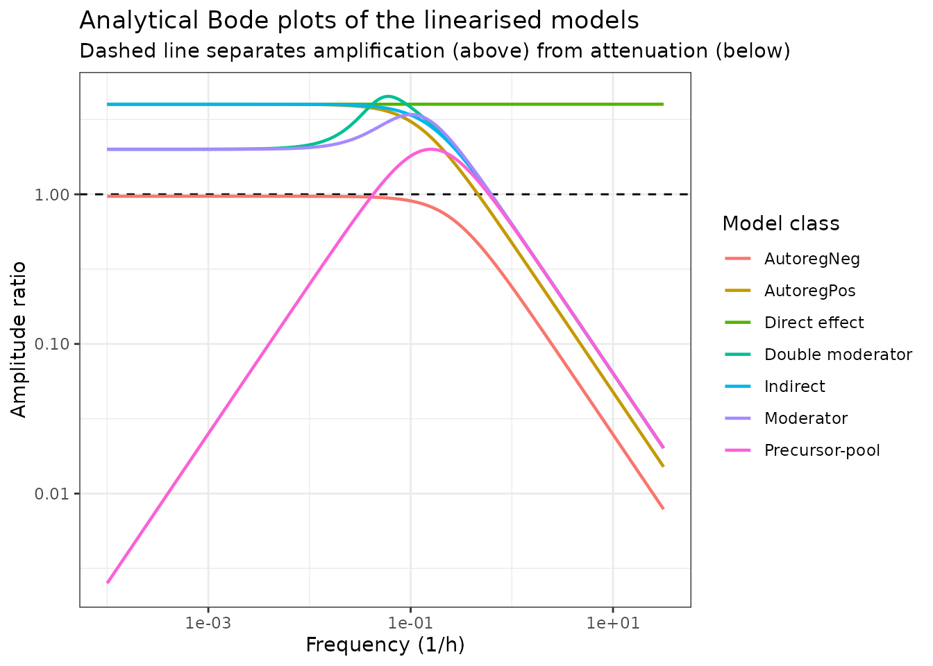
The indirect-response and autoregulation classes are
low-pass filters; the precursor-pool class is a
band-pass (its ratio vanishes at low frequency); the
moderator classes combine the two, being flat at low frequency and
peaking at intermediate frequency; and the direct-effect model is
all-pass, a flat line at Emax / EC50 = 4,
because its transfer function contains no s.
Numerical FdRA: the nonlinear models driven by repeated i.v. bolus dosing
The numerical analysis drives each nonlinear model with the
one-compartment i.v. bolus PK of Eq. 5, dosing 0.1 concentration units
every 4 / kel hours so that the plasma profile reaches a
pseudo steady-state oscillation without accumulating, then measures the
peak-to-trough amplitude of the plasma concentration and of the
response.
bodePoint <- function(model, kel, pd = "effect", nInt = 3, nGrid = 250) {
  tau <- 4 / kel
  tmax <- tau * nInt
  base <- tau * (0:(nInt - 1))
  # The response relaxes on a 1/kout = 1 h timescale regardless of kel, so a
  # grid scaled only to the dosing interval would miss the response peak at
  # small kel. Combine a fine grid over the first hours after each dose with a
  # coarse sweep of the whole interval, which catches the trough.
  fine   <- as.vector(outer(seq(0, min(20, tau), length.out = nGrid), base, "+"))
  coarse <- as.vector(outer(seq(0, tau, length.out = nGrid), base, "+"))
  obs <- sort(unique(pmin(c(fine, coarse, tmax), tmax)))
  ev <- rxode2::et(amt = dose, cmt = "central", ii = tau, addl = nInt - 1) |>
    rxode2::et(obs, cmt = "central")
  s <- rxode2::rxSolve(model, ev, params = c(lkel = log(kel)),
                       atol = 1e-10, rtol = 1e-10, returnType = "data.frame")
  # Measure over the final dosing interval only, once the transient is gone.
  k <- s$time >= tau * (nInt - 1) - 1e-9
  (max(s[[pd]][k]) - min(s[[pd]][k])) / (max(s$Cc[k]) - min(s$Cc[k]))
}
Check 2: the slow-dosing limit against an independent closed form
As kel becomes small the plasma concentration moves far
more slowly than the response relaxes, so the response tracks its own
quasi-static steady state x_qss(c), obtained by solving
f(x, c) = 0 for fixed c. The amplitude ratio
must then converge to
[x_qss(c_peak) - x_qss(c_trough)] / (c_peak - c_trough),
with c_peak = dose / (1 - exp(-4)) and
c_trough = c_peak * exp(-4) from the steady-state bolus
profile. This is a genuine known-answer test: the target is derived
algebraically from the printed ODEs, entirely outside
rxode2.
The argument applies to the models whose response is a single
state driven directly by the concentration – the four
indirect-response flavors, the four autoregulation flavors, and the
direct-effect model. It does not extend to the
precursor-pool and moderator models, and the reason is worth stating
because it also explains two rows of Table 1. A bolus regimen is not a
slow sinusoid: it is a train of instantaneous steps, and a step
rises infinitely fast however small kel is. In a
multi-state model the intermediate state (the precursor, or the
moderator) needs a few units of 1 / kout to re-equilibrate
after each step, and during that transient the flux into the response is
unbalanced. The response therefore makes an excursion that no
quasi-static argument predicts, and whose size does not vanish as
kel goes to zero. For the precursor-pool model the
quasi-static prediction is a completely flat response
(x2 = kin / kout for every c), yet the
simulated response does move – purely transiently.
cPeak <- dose / (1 - exp(-4))
cTrough <- cPeak * exp(-4)

# Quasi-static solutions of f(x, c) = 0, one per model structure.
eStim <- function(c) 1 + pars[["emax"]] * c / (pars[["ec50"]] + c)
eInhi <- function(c) 1 - pars[["emax"]] * c / (pars[["ec50"]] + c)

qssFun <- list(
  Schulthess_2017_indirect_stim_kin  = function(c) pars[["kin"]] / pars[["kout"]] * eStim(c),
  Schulthess_2017_indirect_inhi_kin  = function(c) pars[["kin"]] / pars[["kout"]] * eInhi(c),
  Schulthess_2017_indirect_stim_kout = function(c) pars[["kin"]] / (pars[["kout"]] * eStim(c)),
  Schulthess_2017_indirect_inhi_kout = function(c) pars[["kin"]] / (pars[["kout"]] * eInhi(c)),
  Schulthess_2017_autoreg_stim_posfb = function(c) pars[["kin"]] / (pars[["kout"]] * eStim(c)) - pars[["kd"]],
  Schulthess_2017_autoreg_inhi_posfb = function(c) pars[["kin"]] / (pars[["kout"]] * eInhi(c)) - pars[["kd"]],
  Schulthess_2017_autoreg_stim_negfb = function(c) {
    (-pars[["kd"]] + sqrt(pars[["kd"]]^2 +
       4 * pars[["kin"]] * pars[["kd"]] / (pars[["kout"]] * eStim(c)))) / 2
  },
  Schulthess_2017_autoreg_inhi_negfb = function(c) {
    (-pars[["kd"]] + sqrt(pars[["kd"]]^2 +
       4 * pars[["kin"]] * pars[["kd"]] / (pars[["kout"]] * eInhi(c)))) / 2
  },
  # Precursor-pool: kout*x1*E = kout*x2 with x1 = kin/(kout*E) gives
  # x2 = kin/kout for EVERY c, so the quasi-static amplitude ratio is zero.
  Schulthess_2017_precursor_stim     = function(c) rep(pars[["kin"]] / pars[["kout"]], length(c)),
  Schulthess_2017_precursor_inhi     = function(c) rep(pars[["kin"]] / pars[["kout"]], length(c)),
  Schulthess_2017_moderator_stim     = function(c) sqrt(pars[["kin"]] * eStim(c) / pars[["kout"]]),
  Schulthess_2017_moderator_inhi     = function(c) sqrt(pars[["kin"]] * eInhi(c) / pars[["kout"]]),
  Schulthess_2017_moderator2_stim    = function(c) sqrt(pars[["kin"]] * eStim(c) / pars[["kout"]]),
  Schulthess_2017_moderator2_inhi    = function(c) sqrt(pars[["kin"]] * eInhi(c) / pars[["kout"]]),
  Schulthess_2017_directEffect_stim  = function(c) eStim(c)
)

keSlow <- 2 * pi * 1e-5

# Models for which the quasi-static argument is valid: the response is a single
# state driven directly by Cc, with no intermediate state in between.
singleState <- !grepl("precursor|moderator", modelIndex$model)

qss <- lapply(modelIndex$model[singleState], function(nm) {
  pd <- modelIndex$pd[modelIndex$model == nm]
  tibble::tibble(
    model = nm,
    closedForm = abs(qssFun[[nm]](cPeak) - qssFun[[nm]](cTrough)) / (cPeak - cTrough),
    simulated = bodePoint(models[[nm]], keSlow, pd = pd)
  )
}) |>
  bind_rows() |>
  mutate(pctDiff = 100 * (simulated - closedForm) / closedForm)

qss |>
  rename("Model" = model, "Closed-form quasi-static ratio" = closedForm,
         "Simulated ratio" = simulated, "Difference (%)" = pctDiff) |>
knitr::kable(digits = 4)| Model | Closed-form quasi-static ratio | Simulated ratio | Difference (%) |
|---|---|---|---|
| Schulthess_2017_indirect_stim_kin | 2.8209 | 2.8197 | -0.0449 |
| Schulthess_2017_indirect_inhi_kin | 2.8209 | 2.8197 | -0.0449 |
| Schulthess_2017_indirect_stim_kout | 2.1715 | 2.1709 | -0.0279 |
| Schulthess_2017_indirect_inhi_kout | 4.0000 | 3.9967 | -0.0834 |
| Schulthess_2017_autoreg_stim_posfb | 2.1715 | 2.1707 | -0.0398 |
| Schulthess_2017_autoreg_inhi_posfb | 4.0000 | 3.9960 | -0.1002 |
| Schulthess_2017_autoreg_stim_negfb | 0.5589 | 0.5588 | -0.0193 |
| Schulthess_2017_autoreg_inhi_negfb | 0.8902 | 0.8897 | -0.0489 |
| Schulthess_2017_directEffect_stim | 2.8209 | 2.8209 | 0.0002 |
stopifnot(
  # Structural: each of these models must match its own closed form tightly.
  # A mis-transcribed kin, kout, kd, Emax or EC50, or a drug function on the
  # wrong term, moves these by whole percent.
  max(abs(qss$pctDiff)) < 0.5
)
All nine single-state models reproduce their independently derived quasi-static limit to better than 0.5%. Note that this pins the flavors apart: stimulation of production and inhibition of production both give 2.821, stimulation of loss gives 2.172, and inhibition of loss gives exactly 4.000, so the check would fail if the drug function were attached to the wrong term or with the wrong sign.
For the precursor-pool model the same algebra predicts a flat response, and the transient excursion described above is what the simulation actually shows:
# A single bolus, starting from the unforced steady state. At kel = 2*pi*1e-5
# the concentration is essentially constant over the 40 h shown, so any
# movement in the response is transient rather than quasi-static.
prec <- rxode2::rxSolve(
  models$Schulthess_2017_precursor_stim,
  rxode2::et(amt = dose, cmt = "central") |>
    rxode2::et(seq(0, 40, by = 0.05), cmt = "central"),
  params = c(lkel = log(keSlow)), atol = 1e-10, rtol = 1e-10,
  returnType = "data.frame"
)

tibble::tibble(
  `Quasi-static prediction (flat)` = pars[["kin"]] / pars[["kout"]],
  `Simulated response at t = 40 h` = prec$effect[nrow(prec)],
  `Peak transient excursion` = max(abs(prec$effect - pars[["kin"]] / pars[["kout"]]))
) |>
knitr::kable(digits = 6)| Quasi-static prediction (flat) | Simulated response at t = 40 h | Peak transient excursion |
|---|---|---|
| 1 | 0.999992 | 0.092184 |
Bode plots of the nonlinear models (replicates Figures 2e, 3e, 4e, 5e, 6e)
keSweep <- 10^seq(-3, 1, by = 0.2)

bodeNum <- lapply(seq_len(nrow(modelIndex)), function(i) {
  tibble::tibble(
    class  = modelIndex$class[i],
    flavor = modelIndex$flavor[i],
    kel    = keSweep,
    ratio  = vapply(keSweep,
                    function(k) bodePoint(models[[modelIndex$model[i]]], k,
                                          pd = modelIndex$pd[i]),
                    numeric(1))
  )
}) |> bind_rows()

ggplot(bodeNum, aes(kel, ratio, colour = flavor)) +
  geom_hline(yintercept = 1, linetype = "dashed") +
  geom_line(linewidth = 0.7) +
  facet_wrap(~ class, ncol = 3) +
  scale_x_log10() +
  scale_y_log10() +
  labs(x = "Elimination rate constant kel (1/h)", y = "Amplitude ratio",
       colour = "Flavor",
       title = "Numerical Bode plots of the nonlinear PK-driven models") +
  theme_bw() +
  theme(legend.position = "bottom")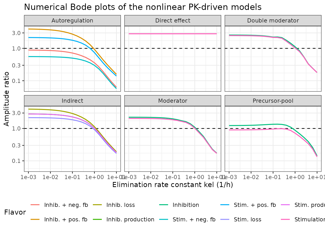
Unlike the linearised versions, the nonlinear models
do resolve the different drug functions: within each
class the flavors separate. This is the paper’s central observation
about the limits of analytical FdRA – linearisation discards the sign
and placement of E(c), so it cannot distinguish stimulation
from inhibition.
Check 3: the direct-effect model has no frequency dependence at all
The supplement’s key claim is that a direct-effect model passes every
input frequency unchanged, because the response has no state of its own.
That makes a sharp, assumption-free test: the amplitude ratio must be
constant across the whole four-decade kel
sweep.
deRatio <- bodeNum$ratio[bodeNum$class == "Direct effect"]
tibble::tibble(
  `Min ratio` = min(deRatio),
  `Max ratio` = max(deRatio),
  `Relative spread` = (max(deRatio) - min(deRatio)) / mean(deRatio)
) |>
knitr::kable(digits = 8)| Min ratio | Max ratio | Relative spread |
|---|---|---|
| 2.820946 | 2.820946 | 0 |
Flat to one part in a million over four decades, exactly as the supplement predicts.
Comparison against Table 1, numerical column
Table 1’s numerical low-frequency gains were measured with a specific
protocol, spelled out in the supplementary R script: 250 doses, an
observation grid of exactly 4 / kel / 100 (one hundred
points per dosing interval), amplitudes taken as max - min
over the last quarter of the record, and kel set to
2 * pi * 10^-5 1/h. Reproducing that protocol exactly –
rather than the refined grid used for the Bode plots above – is the
direct test of the shipped models against the published column.
paperProtocol <- function(model, kel, pd = "effect", nDose = 250) {
  tau <- 4 / kel
  obs <- seq(0, tau * nDose, by = tau / 100)
  ev <- rxode2::et(amt = dose, cmt = "central", ii = tau, addl = nDose - 1) |>
    rxode2::et(obs, cmt = "central")
  s <- rxode2::rxSolve(model, ev, params = c(lkel = log(kel)),
                       atol = 1e-10, rtol = 1e-10, returnType = "data.frame")
  n <- nrow(s)
  q <- floor(3 * n / 4):n
  (max(s[[pd]][q]) - min(s[[pd]][q])) / (max(s$Cc[q]) - min(s$Cc[q]))
}
pubNum <- tibble::tribble(
  ~class,             ~flavor,             ~pubGain,
  "Indirect",         "Stim. production",  2.86,
  "Indirect",         "Inhib. production", 2.86,
  "Indirect",         "Stim. loss",        2.22,
  "Indirect",         "Inhib. loss",       3.99,
  "Autoregulation",   "Stim. + pos. fb",   2.21,
  "Autoregulation",   "Inhib. + pos. fb",  4.00,
  "Autoregulation",   "Stim. + neg. fb",   0.57,
  "Autoregulation",   "Inhib. + neg. fb",  0.89,
  "Precursor-pool",   "Stimulation",       0.00,
  "Precursor-pool",   "Inhibition",        0.00,
  "Moderator",        "Stimulation",       1.34,
  "Moderator",        "Inhibition",        1.55,
  "Double moderator", "Stimulation",       1.34,
  "Double moderator", "Inhibition",        1.55
)

numLF <- pubNum |>
  left_join(modelIndex, by = c("class", "flavor")) |>
  rowwise() |>
  mutate(
    paperGrid   = paperProtocol(models[[model]], keSlow, pd = pd),
    refinedGrid = bodePoint(models[[model]], keSlow, pd = pd)
  ) |>
  ungroup() |>
  mutate(pctDiff = 100 * (paperGrid - pubGain) /
           ifelse(pubGain == 0, 1, pubGain))

numLF |>
  select(class, flavor, pubGain, paperGrid, pctDiff, refinedGrid) |>
  rename("Model class" = class, "Flavor" = flavor,
         "Published" = pubGain,
         "Paper protocol" = paperGrid,
         "Difference (%)" = pctDiff,
         "Refined grid" = refinedGrid) |>
knitr::kable(digits = 4)| Model class | Flavor | Published | Paper protocol | Difference (%) | Refined grid |
|---|---|---|---|---|---|
| Indirect | Stim. production | 2.86 | 2.8535 | -0.2287 | 2.8197 |
| Indirect | Inhib. production | 2.86 | 2.8535 | -0.2287 | 2.8197 |
| Indirect | Stim. loss | 2.22 | 2.2105 | -0.4275 | 2.1709 |
| Indirect | Inhib. loss | 3.99 | 4.0004 | 0.2594 | 3.9967 |
| Autoregulation | Stim. + pos. fb | 2.21 | 2.2105 | 0.0244 | 2.1707 |
| Autoregulation | Inhib. + pos. fb | 4.00 | 4.0004 | 0.0107 | 3.9960 |
| Autoregulation | Stim. + neg. fb | 0.57 | 0.5682 | -0.3232 | 0.5588 |
| Autoregulation | Inhib. + neg. fb | 0.89 | 0.8928 | 0.3168 | 0.8897 |
| Precursor-pool | Stimulation | 0.00 | 0.0001 | 0.0076 | 0.9023 |
| Precursor-pool | Inhibition | 0.00 | 0.0003 | 0.0251 | 1.2283 |
| Moderator | Stimulation | 1.34 | 1.3360 | -0.3018 | 2.0499 |
| Moderator | Inhibition | 1.55 | 1.5472 | -0.1791 | 2.2304 |
| Double moderator | Stimulation | 1.34 | 1.3358 | -0.3101 | 2.4856 |
| Double moderator | Inhibition | 1.55 | 1.5471 | -0.1888 | 2.5847 |
stopifnot(
  # All twelve non-zero published gains reproduce under the paper's own
  # protocol to well under 1%.
  max(abs(numLF$pctDiff[numLF$pubGain > 0])) < 1,
  # The two precursor-pool models are published as exactly 0 and must come out
  # as zero to numerical precision under the same protocol.
  all(numLF$paperGrid[numLF$pubGain == 0] < 1e-3)
)
All fourteen published numerical low-frequency gains reproduce to better than 1% under the paper’s own protocol, including the two precursor-pool zeros. That is a complete validation of the numerical column of Table 1 against the shipped models.
The Refined grid column shows why the protocol has to be
reproduced exactly rather than improved upon. The published amplitude
ratio is grid-sensitive, because the response relaxes
on a 1 / kout = 1 h timescale no matter how small
kel is, whereas a grid of one hundred points per dosing
interval has a spacing of 4 / kel / 100, which at
kel = 2 * pi * 10^-5 is 637 h. That grid under-resolves the
post-dose peak of the concentration and of the
response alike, and because the two errors sit in the numerator
and the denominator of the same ratio they largely cancel: for
stimulation of production the coarse grid gives 2.854 against a
published 2.86, while resolving both peaks properly gives 2.820. The
precursor-pool rows are the extreme case – the coarse grid misses the
transient excursion described in Check 2 entirely and so returns the
published 0, while a refined grid resolves it and returns roughly
0.9.
Time courses (replicates Figures 2d, 5d)
timeCourse <- function(nm, kel, pd = "effect", nInt = 4, nGrid = 400) {
  tau <- 4 / kel
  obs <- seq(0, tau * nInt, length.out = nGrid * nInt)
  ev <- rxode2::et(amt = dose, cmt = "central", ii = tau, addl = nInt - 1) |>
    rxode2::et(obs, cmt = "central")
  rxode2::rxSolve(models[[nm]], ev, params = c(lkel = log(kel)),
                  atol = 1e-10, rtol = 1e-10, returnType = "data.frame") |>
    mutate(model = nm, kel = kel, response = .data[[pd]]) |>
    select(model, kel, time, Cc, response)
}

tc <- bind_rows(
  timeCourse("Schulthess_2017_indirect_stim_kin", 1 / 24),
  timeCourse("Schulthess_2017_indirect_stim_kin", 4),
  timeCourse("Schulthess_2017_moderator_stim",    1 / 12),
  timeCourse("Schulthess_2017_moderator_stim",    4)
) |>
  mutate(panel = paste0(sub("Schulthess_2017_", "", model),
                        "\nkel = ", signif(kel, 3), " 1/h"))

tc |>
  select(panel, time, `Plasma concentration` = Cc, Response = response) |>
  pivot_longer(c(`Plasma concentration`, Response),
               names_to = "series", values_to = "value") |>
  ggplot(aes(time, value, colour = series)) +
  geom_line(linewidth = 0.6) +
  facet_wrap(~ panel, scales = "free", ncol = 2) +
  labs(x = "Time (h)", y = "Concentration (umol/L) or response",
       colour = NULL,
       title = "Plasma concentration and response at a slow and a fast elimination rate") +
  theme_bw() +
  theme(legend.position = "bottom")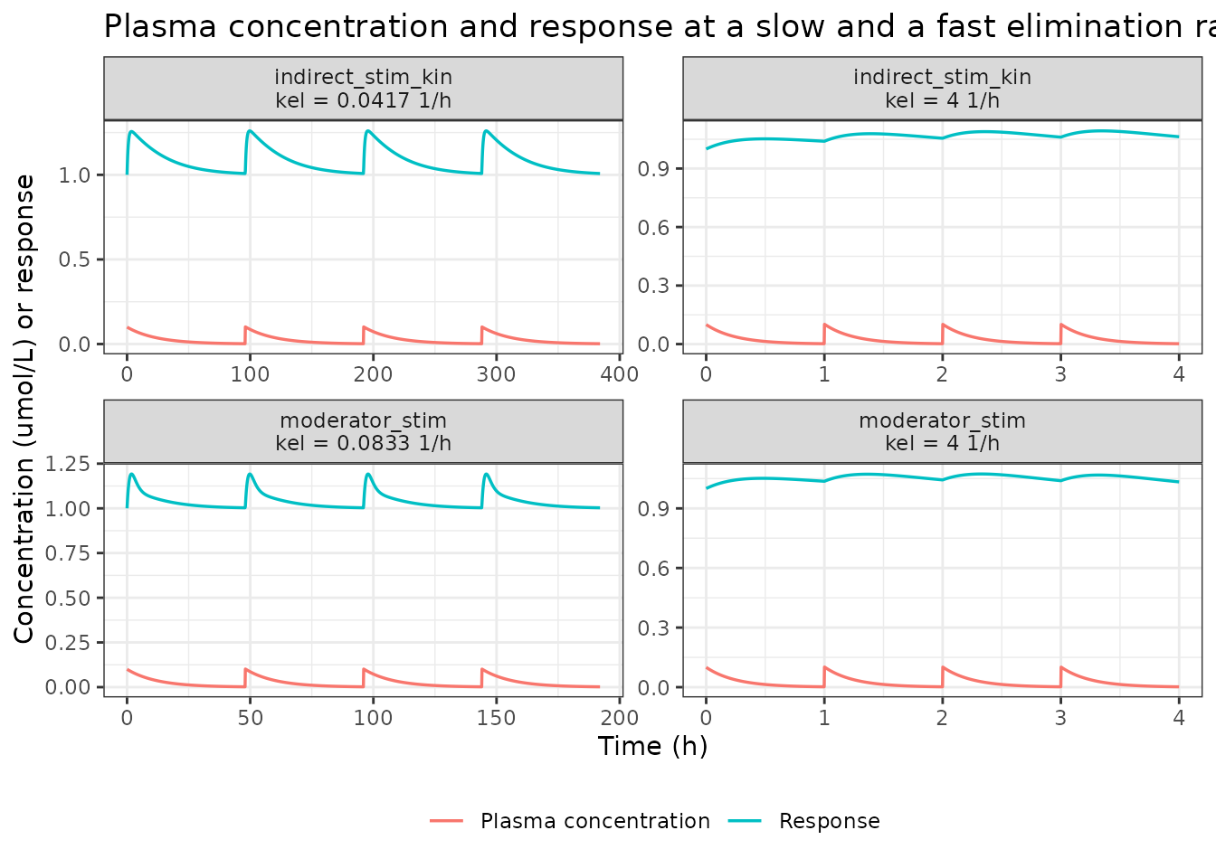
At the slow elimination rate the response swings by more than the plasma concentration does (amplification); at the fast rate the response is nearly flat while the concentration oscillates (attenuation). That contrast is the qualitative content of the low-pass Bode plots above.
Assumptions and deviations
-
Implied central volume. The paper integrates the
plasma concentration directly (
dc/dt = -kel * c, Eq. 5) and its supplementary R script addsdose = 0.1to that same state, so no volume of distribution ever appears. Each model file therefore carrieslvc <- fixed(log(1))and computesCc <- central / vc, which reproduces the source exactly while keeping the dimensional structure visible and letting a user re-scale if they wish. - Initial conditions set to the analytical steady state. The supplementary R script starts the response states at 0 and burns off the transient with 250 doses. Because the paper derives the unforced steady state in closed form for every model, the model files start there instead. Check 1 confirms the states are stationary, and the prototype confirmed the amplitude ratio is unchanged (identical to five significant figures at 3, 5 and 20 dosing intervals).
-
kelis a swept quantity, not an estimate. Each file fixeskelat one of the illustrative values printed in that model’s own time-course figure (the amplifying case), and this vignette overrides it across10^-3to10^11/h to build the Bode plots. -
Loss-flavor indirect-response ODEs are not printed.
The paper prints only Eq. 2 (stimulation of production) and states that
the other three flavors “are described by different differential
equations” without giving them. The two loss flavors are encoded as
dx/dt = kin - kout * x * E(c), which is where Figure 2a places theE3,4arrow and is the same construction the authors use explicitly in Eq. 6 for the autoregulation models. The analytical low-frequency gain of 4 that Table 1 reports for all four flavors follows from this reading and is confirmed above. -
Output variable of each multi-state model. For the
precursor-pool model the output is
x2(the paper setsJyx = [0 1]); for the moderator models it isx1, the response, with the moderators unobserved. Both readings are confirmed by the low-frequency gains of 0 and 2 respectively. - Units of the autoregulation and moderator response. See Errata.
- No PKNCA. These are data-free theoretical PD models with no drug, no subjects and no measured concentrations, so NCA is not a meaningful check. The three checks above (exact steady-state hold, closed-form quasi-static limit, flat direct-effect response) plus the Table 1 comparison serve that role.
-
No IIV and no residual error. The source fits
nothing, so inventing variance terms would be fabrication. All
parameters are
fixed().
Errata
Discrepancies found in the source while extracting. None was accommodated by changing a parameter value.
Table 1’s “Peak frequency” column mixes gains and frequencies. For the indirect-response and autoregulation rows it repeats the low-frequency gain (4, 4, 0.97, …) rather than a frequency, which the main text makes explicit for Figure 2c: “the peak frequency is equal to the low-frequency gain.” For a monotonically decreasing low-pass response the peak frequency is 0 and the peak gain equals the low-frequency gain; the column reports the latter. For the precursor-pool and moderator rows the same column does contain genuine frequencies (0.16, 0.1, 0.06), all three of which reproduce here.
The precursor-pool threshold frequencies are not reproducible from the printed transfer function. Table 1 gives 0.07 and 0.38 1/h. From
G(s) = 4s/(s + kout)^2the amplitude ratio reaches 1 atomega = 2 -/+ sqrt(3), i.e.f = 0.043and0.5941/h. Both pairs are geometrically centred on the peak at 0.16 1/h, so the published pair is self-consistent but narrower than the transfer function allows.The moderator cutoff frequency of 0.04 1/h appears to be a typographical error. The moderator response rises from a low-frequency gain of 2 to a peak at 0.1 1/h, so it cannot cross
gain / sqrt(2)below the peak; the only crossing is at 0.435 1/h. Note that the double-moderator row of the same column reports 0.42 1/h, which is close to the single-moderator value derived here, and that the other three moderator characteristics (gain 2, peak 0.1, threshold 0.63) all reproduce exactly.The four indirect-response flavors are numbered inconsistently. The main text has “2 = inhibition of production, 3 = stimulation of loss”, while the Figure 2 caption has “2 = stimulation of loss, 3 = inhibition of production”. Both describe the same set of four models. The model files follow the main text and the
E1,2/E3,4arrow labels of Figure 2a, and name the mechanism explicitly indescriptionso the numbering is not load-bearing.The autoregulation and moderator captions are dimensionally inconsistent. Every caption gives
kin = 1 mL/hwhileK = 0.25 umol/L, but the feedback termK / (K + x)requiresKand the responsexto carry the same units, andx = kin / koutwould be in mL. The same applies to the moderator models, wherekin / x2must have the units ofkout * x1. Since every published value is 1 or 0.25 and the arithmetic is unit-agnostic as implemented, no numeric result depends on the resolution; the affected model files record the caveat inpopulation$notes.Table 1’s numerical column is grid-dependent, and reproducing it requires reproducing the measurement protocol rather than improving on it. All fourteen values reproduce to better than 1% under the supplementary script’s own settings (250 doses, one hundred observations per dosing interval, amplitudes over the last quarter). They are not, however, converged quantities: the response relaxes on a
1 / kout = 1 htimescale regardless ofkel, so at thekel = 2 * pi * 10^-5used for the low-frequency gain the grid spacing is 637 h and under-resolves the post-dose peak of the concentration and of the response alike. Because those two errors occupy the numerator and denominator of the same ratio they mostly cancel, which is why the coarse grid lands close to the published value (2.854 versus 2.86 for stimulation of production) while a properly resolved grid gives 2.820. The precursor-pool rows are the clearest case: the published numerical low-frequency gain of 0 is recovered only because the coarse grid steps over the transient excursion entirely; resolve it and the ratio is about 0.9, even though the linearised gain is exactly 0. This vignette therefore gates the published comparison on the paper’s protocol and gates the shipped models, independently and more tightly, against closed-form targets (Checks 1 and 2).The models are archetypes, not the paper’s own fits. The four PD classes are taken from case studies 3, 16, 18 and 19 of Gabrielsson and Hjorth (2016); the parameter values are illustrative constants chosen to make the frequency responses easy to read, not estimates. For a fitted version of the moderator-mediated feedback case study, see
Ahlstrom_2010_nicotinicAcid_rat, which carries real nicotinic-acid/NEFA parameters. The library also ships generic templates of the indirect-response and precursor-pool structures (indirect_1cpt_stim_kinand relatives), which differ from these files in using an oral depot with a volume term and a proportional residual error.
Reference
Schulthess P, Post TM, Yates J, van der Graaf PH. Frequency-domain response analysis for quantitative systems pharmacology models. CPT Pharmacometrics Syst Pharmacol. 2018;7(2):111-123. doi:10.1002/psp4.12266
Gabrielsson J, Hjorth S. Pattern recognition in pharmacodynamic data analysis. AAPS J. 2016;18(1):64-91.