Erythropoiesis and CKD anemia QSP model (Roy 2023)
Source:vignettes/articles/Roy_2023_erythropoiesis_qsp.Rmd
Roy_2023_erythropoiesis_qsp.RmdModel and source
- Citation: Roy M, Saroha S, Sarma U, Sarathy H, Kumar R. Quantitative systems pharmacology model of erythropoiesis to simulate therapies targeting anemia due to chronic kidney disease. Front Pharmacol. 2023;14:1274490. doi:10.3389/fphar.2023.1274490. Equations 1-28 are from the main text section 3.3; the expanded PHD and progenitor-apoptosis Hill forms and the EPO molecule unit conversion are from the Supplementary Appendix (‘Detailed Equations’). Every parameter value, unit and per-CKD-stage alternate parameterization is from the Supplementary ‘Parameter Dashboard’ (Table1.XLSX, sheets ‘Parameters’ and ‘Species’). Reaction stoichiometry, rate laws and assignment rules were read from the authors’ own SimBiology project released as Supplementary DataSheet1.ZIP, file ‘Model File and Scripts/ErythropoiesisModel_5Aug2023_Final3.sbproj’.
- Article: https://doi.org/10.3389/fphar.2023.1274490
Roy, Saroha, Sarma, Sarathy and Kumar (Frontiers in Pharmacology, 2023) describe a quantitative systems pharmacology (QSP) model of human erythropoiesis and of its disruption in anemia due to chronic kidney disease (CKD). The model closes the physiological negative-feedback loop Hb -> prolyl hydroxylase (PHD) -> HIF-alpha -> renal EPO -> erythroid progenitor survival -> reticulocytes -> RBC -> Hb, and adds four therapies: the erythropoiesis-stimulating agents (ESAs) recombinant human EPO (epoetin alfa) and darbepoetin alfa, and the oral HIF prolyl-hydroxylase inhibitors (PHIs) vadadustat and daprodustat.
This is a deterministic, typical-individual mechanism
model. The paper reports no IIV and no residual-error model:
population variability is produced by log-normal resampling of five
sensitive parameters around a reference virtual patient, not by an omega
matrix. Accordingly the model file carries no eta terms and
no residual error, and this vignette validates it with steady-state,
mass-balance, dimensional-analysis and published-response checks rather
than with PKNCA.
mod <- readModelDb("Roy_2023_erythropoiesis_qsp")Population
Anemia due to chronic kidney disease. Five reference virtual patients span healthy and CKD stages 1.5, 3, 4 and 5. Virtual populations are of two kinds: non-dialysis (ND; CKD stages 3, 4 and 5, erythropoiesis-stimulating-agent naive, built around a CKD 4 reference patient) and hemodialysis (HD; CKD stage 5 only, previously treated with rHuEPO, built around a CKD 5 reference patient). Iron sufficiency is assumed throughout.
The calibration set is ten clinical trials (Tables 1 and 2 of the paper): PK from Cheung 2001 (rHuEPO), Kim 2019 (darbepoetin), Chavan 2021 (vadadustat) and Yamada 2020 (daprodustat); Hb response from Provenzano 2004 and Nissenson 2002 (rHuEPO), Suranyi 2003 and Locatelli 2003 (darbepoetin), Pergola 2016 and Haase 2019 (vadadustat), and Holdstock 2019 and Meadowcroft 2019 (daprodustat). Pergola 2009 (rHuEPO QW / Q2W / TIW) is held out for validation. Steady-state Hb, EPO, reticulocyte and RBC ranges by CKD stage (Figure 3) come from Li 2019 and Sheth & Shah 2016.
Source trace
Every model element and its location in the source. The paper prints
the ODE system as Equations 1-28 but tabulates no parameter
values in the main text; all values come from the Supplementary
“Parameter Dashboard” (Table1.XLSX). Reaction stoichiometry
and the exact rate laws were read from the authors’ own SimBiology
project, released as Supplementary DataSheet1.ZIP
(ErythropoiesisModel_5Aug2023_Final3.sbproj).
| Model element | Source location |
|---|---|
PHD assignment (Hb and PHI effects) |
Eq. 1; expanded in Suppl. “Detailed Equations”; sbproj
rule_14 |
d/dt(HIFa) |
Eq. 2-3; sbproj reaction_3, reaction_4 |
| EPO production Hill | Eq. 4; sbproj reaction_5 |
| EPO plasma clearance / distribution | Eq. 5-6, 10-11; sbproj reaction_22, reaction_23 |
| EPO-EPOR binding, EPOR recycling | Eq. 7-9, 12-13; sbproj reaction_8_1, reaction_8,
reaction_11, reaction_28 |
| EPO ng/mL -> molecule/mL conversion | Suppl. “Detailed Equations” (EPO_plasma/MW_EPO) |
| Progenitor production / maturation / apoptosis | Eq. 14-17; sbproj reaction_13, reaction_14,
reaction_7 |
| 4th-order progenitor-rescue Hill | Suppl. “Detailed Equations”; sbproj reaction_7 |
| Precursor amplification factor 32 |
sbproj reaction_29 (not stated in the main text; see
Errata) |
| Precursor / reticulocyte / RBC chain | Eq. 18-27; sbproj reaction_18, reaction_1, reaction_15,
reaction_26, reaction_19 |
HGB assignment |
Eq. 28; sbproj rule_1 |
EPO_plasma_IU, RBC_total
|
sbproj rule_2, rule_5 |
| rHuEPO PK (SC absorption, TMDD) | Section 3.3.5; sbproj reaction_16, reaction_25,
reaction_24, reaction_2, reaction_2_1, reaction_12 |
| Darbepoetin PK/binding | Section 3.3.5-3.3.6; sbproj reaction_32, reaction_30,
reaction_31, reaction_6, reaction_2_2, reaction_33 |
| PHI PK (oral, linear + saturable) | Section 3.3.5; sbproj reaction_17, reaction_20,
reaction_21, reaction_9 |
| All parameter values and units | Suppl. Parameter Dashboard, sheet “Parameters” |
| All initial conditions | Suppl. Parameter Dashboard, sheet “Species” |
| Five CKD-stage parameterizations | Suppl. Parameter Dashboard, per-stage columns; Suppl. Table S1 |
Units table (dimensional analysis)
Mechanistic models mix per-mL and per-L quantities, so every ODE term is checked explicitly.
| Quantity | Units |
|---|---|
HIFa, EPO_plasma,
rhuEPO_plasma, Darbe_plasma,
PHI_Plasma, PHD
|
ng/mL |
Progenitors, Precursors,
Retics_plasma, RBCM,
EPO_receptor, *_LR_complex
|
molecule/L |
rhuEPO_SC_Dose, darbe_SC_Dose
|
ng (amount) |
PHI_Dose_Gut |
ug (amount) |
HGB |
g/dL |
EPO_plasma_IU |
milliU/mL |
MW_EPO, MW_ESA
|
ng/molecule |
kon_* |
L/(molecule*h) |
all k* rate constants |
1/h |
CLD_PHI |
mL/h |
Vc, Vp
|
L |
Two conversions are implicit in the released SimBiology rate laws because that project runs with unit conversion enabled; the model file writes them out.
-
mLperLon the receptor-binding limb.EPO_plasma / MW_EPOhas units (ng/mL)/(ng/molecule) = molecule/mL, but it multipliesEPO_receptorin molecule/L, so it is scaled by 1000. The reverse conversion appears on the plasma side of the same reaction: the molecule/(Lh) flux timesMW_EPOgives ng/(Lh), divided by 1000 to give ng/(mL*h). The Supplement states explicitly that “EPO_plasma in the equation is in the units of molecule/mL”, confirming the mismatch is real and is resolved by the platform. -
ngPerUgon the PHI Hill function.scalar_PHI_DRUGcarries units mL/ug, soscalar_PHI_DRUG * PHI_Plasmais dimensionless only if plasma PHI enters in ug/mL, while thePHI_Plasmastate is ng/mL.
Both are load-bearing rather than cosmetic: the section “Why the unit factors are required” below shows that omitting the first makes the entire EPO-EPOR pharmacodynamic limb inert.
Parameter table: paper vs. model file
The five parameters that differ across virtual patients are the disease axis of the model. Values are the Supplementary Parameter Dashboard columns.
stage_par <- tibble::tribble(
  ~Stage,     ~k_production_EPO, ~Km_EPO_EPOR_Progenitors, ~kprod_prog, ~kdeg_RBCM, ~k_deg_prog,
  "Healthy",   2.02,  5.1500e12, 3.60e9, 0.000340, 0.0669,
  "CKD 1.5",   1.85,  4.2014e12, 2.00e9, 0.000370, 0.0525,
  "CKD 3",     1.70,  3.3010e12, 2.10e9, 0.000463, 0.0300,
  "CKD 4",     1.60,  2.5000e12, 1.50e9, 0.000473, 0.0260,
  "CKD 5",     1.30,  2.0000e12, 1.38e9, 0.000694, 0.0158
)
knitr::kable(
  stage_par,
  caption = paste(
    "Per-CKD-stage parameterizations (Supplementary Parameter Dashboard).",
    "The Healthy k_deg_prog is back-solved (see Errata); every other value",
    "is printed in the dashboard. CKD 4 is the non-dialysis reference",
    "virtual patient and is the parameterization shipped in ini()."
  )
)| Stage | k_production_EPO | Km_EPO_EPOR_Progenitors | kprod_prog | kdeg_RBCM | k_deg_prog |
|---|---|---|---|---|---|
| Healthy | 2.02 | 5.1500e+12 | 3.60e+09 | 0.000340 | 0.0669 |
| CKD 1.5 | 1.85 | 4.2014e+12 | 2.00e+09 | 0.000370 | 0.0525 |
| CKD 3 | 1.70 | 3.3010e+12 | 2.10e+09 | 0.000463 | 0.0300 |
| CKD 4 | 1.60 | 2.5000e+12 | 1.50e+09 | 0.000473 | 0.0260 |
| CKD 5 | 1.30 | 2.0000e+12 | 1.38e+09 | 0.000694 | 0.0158 |
kdeg_RBCM is the mechanistic anemia driver most directly
checkable against physiology: 1/kdeg_RBCM is the mean RBC
lifespan, giving 122 days for the healthy patient and 60 days for CKD 5
– reproducing the RBC-lifespan shortening reported by Li 2019, the
paper’s own source for these data.
stage_par |>
  transmute(Stage, `RBC lifespan (days)` = round(1 / kdeg_RBCM / 24, 1)) |>
knitr::kable(caption = "Implied mean RBC lifespan by CKD stage.")| Stage | RBC lifespan (days) |
|---|---|
| Healthy | 122.5 |
| CKD 1.5 | 112.6 |
| CKD 3 | 90.0 |
| CKD 4 | 88.1 |
| CKD 5 | 60.0 |
Simulation helpers
The model’s published initial conditions are the authors’ starting values, not the steady state; the paper runs each virtual patient to steady state before dosing (Methods 3.4.3). Every simulation below therefore equilibrates first. The slowest relaxation time is the RBC lifespan (at most ~122 days), so an 8-year burn-in is more than 20 relaxation times.
stages <- list(
  "Healthy" = c(k_production_EPO = 2.02, Km_EPO_EPOR_Progenitors = 5.15e12,
                kprod_prog = 3.6e9, kdeg_RBCM = 0.00034, k_deg_prog = 0.0669),
  "CKD 3"   = c(k_production_EPO = 1.7, Km_EPO_EPOR_Progenitors = 3.301e12,
                kprod_prog = 2.1e9, kdeg_RBCM = 0.000463, k_deg_prog = 0.03),
  "CKD 4"   = c(k_production_EPO = 1.6, Km_EPO_EPOR_Progenitors = 2.5e12,
                kprod_prog = 1.5e9, kdeg_RBCM = 0.000473, k_deg_prog = 0.026),
  "CKD 5"   = c(k_production_EPO = 1.3, Km_EPO_EPOR_Progenitors = 2.0e12,
                kprod_prog = 1.38e9, kdeg_RBCM = 0.000694, k_deg_prog = 0.0158)
)

# Drug-specific PHI parameter sets (Parameter Dashboard, Vada / Dapro rows)
phi_par <- list(
  vadadustat  = c(Vmax_DRUG_PHD = 1.27, ka_gutToPlasma = 0.36,
                  kel_PHI = 0.1, CLD_PHI = 900,
                  Vmax_nonlinearClearance = 0, Vc = 4.9573),
  daprodustat = c(Vmax_DRUG_PHD = 2.2, ka_gutToPlasma = 0.2239,
                  kel_PHI = 0.025, CLD_PHI = 0.173,
                  Vmax_nonlinearClearance = 115, Vc = 5.38)
)

BURN_H <- 8 * 365 * 24

equilibrate <- function(pars) {
  s <- rxSolve(mod, params = pars, et(c(0, BURN_H)),
               atol = 1e-12, rtol = 1e-10, maxsteps = 1e7)
  last <- tail(s, 1)
  st <- c(HIFa = last$HIFa, EPO_plasma = last$EPO_plasma,
          EPO_periphery = last$EPO_periphery,
          EPO_LR_complex = last$EPO_LR_complex,
          rhuEPO_LR_complex = last$rhuEPO_LR_complex,
          darbe_LR_complex = last$darbe_LR_complex,
          EPO_receptor = last$EPO_receptor,
          rhuEPO_SC_Dose = 0, rhuEPO_plasma = last$rhuEPO_plasma,
          rhuEPO_periphery = last$rhuEPO_periphery,
          darbe_SC_Dose = 0, Darbe_plasma = last$Darbe_plasma,
          darbe_periphery = last$darbe_periphery,
          PHI_Dose_Gut = 0, PHI_Plasma = last$PHI_Plasma,
          PHI_periphery = last$PHI_periphery,
          Progenitors = last$Progenitors, Precursors = last$Precursors,
          Retics_plasma = last$Retics_plasma, RBCM = last$RBCM)
  list(inits = st, hb = last$HGB, epo = last$EPO_plasma_IU,
       retic = last$Retic_pct)
}

# rHuEPO / darbepoetin doses are amounts in ng; scaler_EPO = 119.05 mU/ng.
IU_to_ng <- 1000 / 119.05

dose_run <- function(stage, cmt, amt, ii, n_dose, weeks,
                     extra = NULL, by = 12) {
  pars <- stages[[stage]]
  if (!is.null(extra)) pars <- c(pars, extra)
  eq <- equilibrate(pars)
  ev <- et(amt = amt, cmt = cmt, ii = ii, addl = n_dose - 1, time = 0) |>
    add.sampling(seq(0, weeks * 7 * 24, by = by))
  s <- rxSolve(mod, params = pars, ev, inits = eq$inits,
               atol = 1e-10, rtol = 1e-8, maxsteps = 1e7)
  list(baseline = eq$hb, final = tail(s$HGB, 1),
       delta = tail(s$HGB, 1) - eq$hb, sim = s)
}
1. Steady-state check and Figure 3 replication
Each reference virtual patient is run undosed for eight years. A correct translation holds the paper’s reported baseline indefinitely; the table below compares the resulting Hb and plasma EPO against the ranges the paper shows in Figure 3 (data from Li 2019).
ss <- lapply(names(stages), function(nm) {
  e <- equilibrate(stages[[nm]])
  tibble::tibble(Stage = nm, Hb = e$hb, EPO = e$epo, Retic = e$retic)
}) |> bind_rows()

ss |>
  mutate(
    `Reported Hb (g/dL)` = c("13.5 (Cheung 2001 healthy)", "~12", "~10", "<10"),
    across(c(Hb, EPO, Retic), \(x) round(x, 2))
  ) |>
  rename("Simulated Hb (g/dL)" = Hb,
         "Simulated EPO (mU/mL)" = EPO,
         "Simulated reticulocytes (%)" = Retic) |>
  knitr::kable(
    caption = paste(
      "Steady-state readouts by CKD stage vs. the ranges in Figure 3.",
      "Plasma EPO stays in the normal 7-12 mU/mL band across stages,",
      "reproducing the paper's observation that plasma EPO is not a",
      "reliable marker of CKD anemia severity."
    )
)| Stage | Simulated Hb (g/dL) | Simulated EPO (mU/mL) | Simulated reticulocytes (%) | Reported Hb (g/dL) |
|---|---|---|---|---|
| Healthy | 13.51 | 11.20 | 1.24 | 13.5 (Cheung 2001 healthy) |
| CKD 3 | 12.05 | 9.47 | 1.69 | ~12 |
| CKD 4 | 9.61 | 9.15 | 1.72 | ~10 |
| CKD 5 | 9.11 | 7.48 | 2.51 | <10 |
The model reproduces the central clinical facts of the paper: Hb falls monotonically with CKD stage to below 10 g/dL at CKD 5, while plasma EPO stays within the healthy range – exactly the “CKD 3 or CKD 4 patients may have plasma EPO levels equivalent to those observed in healthy volunteers” observation in Methods 3.4.2. Reticulocyte percentage rises with severity, consistent with Figure 3C.
Steady state is genuine, not a slow transient: re-running the equilibrated CKD 4 patient for a further two years must not move Hb.
eq4 <- equilibrate(stages[["CKD 4"]])
hold <- rxSolve(mod, params = stages[["CKD 4"]],
                et(seq(0, 2 * 365 * 24, by = 24)), inits = eq4$inits,
                atol = 1e-12, rtol = 1e-10, maxsteps = 1e7)
drift <- max(abs(hold$HGB - eq4$hb))
cat(sprintf("Maximum Hb drift over 2 further years: %.3g g/dL\n", drift))
#> Maximum Hb drift over 2 further years: 2.62e-11 g/dL
stopifnot(drift < 1e-3)
2. Mass-balance / flux check
At steady state every flux in the erythroid chain must balance, and
the EPOR pool must be conserved (EPO_receptor + all three
ligand-receptor complexes = 4e13 molecule/L, since
reaction_28 regenerates one free receptor per internalised
complex).
p <- c(as.list(stages[["CKD 4"]]),
       list(k_progenitorsToPrecursors = 0.0046, progenitorAmplification = 32,
            kdeg_Precursors = 0.05, k_PrecursorsToPretics = 0.04,
            k_ReticsToRBCM = 0.027, kdeg_Retics_Plasma = 0.03,
            Vmax_EPO_EPOR_effective = 0.99, nEPO_EPOR_to_Progenitors = 4))
st <- eq4$inits
fEPO <- with(p, Vmax_EPO_EPOR_effective *
               st[["EPO_LR_complex"]]^nEPO_EPOR_to_Progenitors /
               (Km_EPO_EPOR_Progenitors^nEPO_EPOR_to_Progenitors +
                  st[["EPO_LR_complex"]]^nEPO_EPOR_to_Progenitors))

flux <- tibble::tibble(
  State = c("Progenitors", "Precursors", "Retics_plasma", "RBCM"),
  `In (molecule/L/h)` = c(
    p$kprod_prog,
    p$k_progenitorsToPrecursors * st[["Progenitors"]] * p$progenitorAmplification,
    p$k_PrecursorsToPretics * st[["Precursors"]],
    p$k_ReticsToRBCM * st[["Retics_plasma"]]
  ),
  `Out (molecule/L/h)` = c(
    p$k_progenitorsToPrecursors * st[["Progenitors"]] +
      p$k_deg_prog * st[["Progenitors"]] * (1 - fEPO),
    (p$kdeg_Precursors + p$k_PrecursorsToPretics) * st[["Precursors"]],
    (p$k_ReticsToRBCM + p$kdeg_Retics_Plasma) * st[["Retics_plasma"]],
    p$kdeg_RBCM * st[["RBCM"]]
  )
) |>
  mutate(`Relative imbalance` = signif(abs(`In (molecule/L/h)` -
                                             `Out (molecule/L/h)`) /
                                         `In (molecule/L/h)`, 3))
knitr::kable(flux, caption = "Steady-state flux balance in the erythroid chain.")| State | In (molecule/L/h) | Out (molecule/L/h) | Relative imbalance |
|---|---|---|---|
| Progenitors | 1500000000 | 1500000000 | 0 |
| Precursors | 7311641411 | 7311641411 | 0 |
| Retics_plasma | 3249618405 | 3249618405 | 0 |
| RBCM | 1539292929 | 1539292929 | 0 |
stopifnot(all(flux$`Relative imbalance` < 1e-4))

epor_total <- st[["EPO_receptor"]] + st[["EPO_LR_complex"]] +
  st[["rhuEPO_LR_complex"]] + st[["darbe_LR_complex"]]
cat(sprintf("Total EPOR pool: %.6g molecule/L (declared 4e13)\n", epor_total))
#> Total EPOR pool: 4e+13 molecule/L (declared 4e13)
stopifnot(abs(epor_total / 4e13 - 1) < 1e-6)
3. Why the unit factors are required
The mLperL factor on the receptor-binding limb is not
cosmetic. Setting it to 1 – i.e. taking the released rate law at face
value without the platform’s unit conversion – leaves the EPO-EPOR
complex three orders of magnitude below
Km_EPO_EPOR_Progenitors, so the progenitor-rescue Hill
function is pinned at zero and no ESA can produce any Hb response at
all. This check pins the interpretation.
eq_probe <- equilibrate(stages[["CKD 4"]])
lr_ratio <- eq_probe$inits[["EPO_LR_complex"]] /
  stages[["CKD 4"]][["Km_EPO_EPOR_Progenitors"]]
cat(sprintf(
  "Baseline EPO-EPOR complex / Km = %.3g (with mLperL = 1000)\n", lr_ratio))
#> Baseline EPO-EPOR complex / Km = 0.355 (with mLperL = 1000)
cat(sprintf(
  "Without the factor this ratio would be ~%.3g, giving fEPO ~ %.1e\n",
  lr_ratio / 1000, 0.99 * (lr_ratio / 1000)^4))
#> Without the factor this ratio would be ~0.000355, giving fEPO ~ 1.6e-14
With the factor the complex sits at a workable fraction of
Km, so a 4th-order Hill can swing from near-zero at
baseline to the Vmax of 0.99 under ESA – which is precisely
the pharmacodynamic mechanism the paper describes. The therapy
replications below confirm the resulting magnitudes.
4. Reference virtual patient responses to all four therapies
The Supplementary “Developing Virtual Patients” section reports the Hb rise of the non-dialysis reference virtual patient (CKD 4) for each therapy at its calibration dose and duration. These are the paper’s own quantitative targets and are the strongest available end-to-end check.
res <- list(
  list("rHuEPO 10,000 IU QW, 16 wk",  dose_run("CKD 4", "rhuEPO_SC_Dose",
        10000 * IU_to_ng, 168, 16, 16), 2.9),
  list("Darbepoetin 55 ug Q2W, 24 wk", dose_run("CKD 4", "darbe_SC_Dose",
        55e3, 336, 12, 24), 2.6),
  list("Vadadustat 450 mg QD, 19 wk",  dose_run("CKD 4", "PHI_Dose_Gut",
        450e3, 24, 133, 19, extra = phi_par$vadadustat), 1.32),
  list("Daprodustat 4 mg QD, 25 wk",   dose_run("CKD 4", "PHI_Dose_Gut",
        4e3, 24, 175, 25, extra = phi_par$daprodustat), 1.4)
)

therapy <- tibble::tibble(
  Therapy   = vapply(res, \(x) x[[1]], character(1)),
  Baseline  = round(vapply(res, \(x) x[[2]]$baseline, numeric(1)), 2),
  Simulated = round(vapply(res, \(x) x[[2]]$delta, numeric(1)), 2),
  Reported  = vapply(res, \(x) x[[3]], numeric(1))
) |>
  mutate(`Difference (%)` = round(100 * (Simulated - Reported) / Reported, 1))

therapy |>
  rename("Baseline Hb (g/dL)" = Baseline,
         "Simulated dHb (g/dL)" = Simulated,
         "Reported dHb (g/dL)" = Reported) |>
  knitr::kable(
    caption = paste(
      "Hb rise in the non-dialysis (CKD 4) reference virtual patient vs. the",
      "values reported in the Supplementary 'Developing Virtual Patients'",
      "section. rHuEPO and vadadustat reproduce the paper; darbepoetin and",
      "daprodustat do not (see Errata)."
    )
)| Therapy | Baseline Hb (g/dL) | Simulated dHb (g/dL) | Reported dHb (g/dL) | Difference (%) |
|---|---|---|---|---|
| rHuEPO 10,000 IU QW, 16 wk | 9.61 | 2.92 | 2.90 | 0.7 |
| Darbepoetin 55 ug Q2W, 24 wk | 9.61 | 1.01 | 2.60 | -61.2 |
| Vadadustat 450 mg QD, 19 wk | 9.61 | 1.38 | 1.32 | 4.5 |
| Daprodustat 4 mg QD, 25 wk | 9.61 | 1.93 | 1.40 | 37.9 |
The rHuEPO and vadadustat arms reproduce the paper’s reported reference-patient responses to within 5%, which validates the whole coupled system end to end: the erythroid chain including the factor-32 amplification, the TMDD binding limb, the 4th-order rescue Hill, the Hb-PHD-HIF feedback and both PK sub-models.
stopifnot(abs(therapy$Simulated[1] - 2.9)  < 0.15)  # rHuEPO
stopifnot(abs(therapy$Simulated[3] - 1.32) < 0.15)  # vadadustat
traj <- lapply(seq_along(res), function(i) {
  s <- res[[i]][[2]]$sim
  tibble::tibble(Week = s$time / (7 * 24), Hb = s$HGB,
                 Therapy = res[[i]][[1]])
}) |> bind_rows()

ggplot(traj, aes(Week, Hb)) +
  geom_line(linewidth = 0.7, colour = "steelblue") +
  facet_wrap(~Therapy, scales = "free_x") +
  labs(x = "Time (weeks)", y = "Hemoglobin (g/dL)") +
  theme_bw()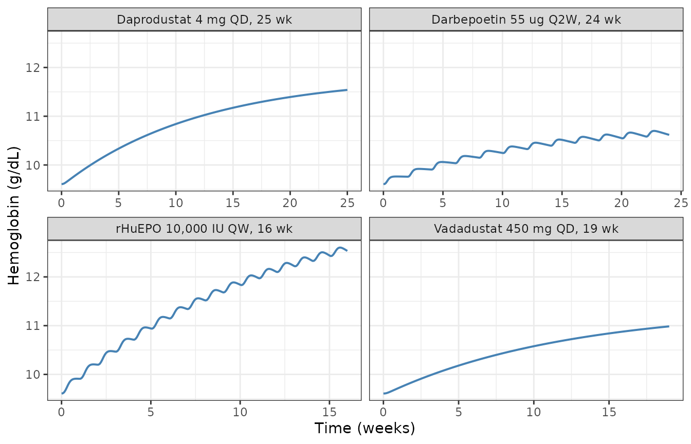
Hb trajectory of the CKD 4 non-dialysis reference virtual patient under each of the four therapies. Replicates Supplementary Figure S2.
5. Healthy volunteer calibration (Cheung 2001)
Table 2 of the paper reports that healthy volunteers given 40,000 IU QW subcutaneous rHuEPO rise from a baseline Hb of 13.5 +/- 0.79 to 16.4 +/- 0.41 g/dL, and the model is calibrated simultaneously to the 40,000 IU QW and 10,500 IU TIW arms.
cheung <- bind_rows(
  {r <- dose_run("Healthy", "rhuEPO_SC_Dose", 40000 * IU_to_ng, 168, 4, 4)
   tibble::tibble(Arm = "40,000 IU QW", Baseline = r$baseline, Final = r$final)},
  {r <- dose_run("Healthy", "rhuEPO_SC_Dose", 10500 * IU_to_ng, 56, 12, 4)
   tibble::tibble(Arm = "10,500 IU TIW", Baseline = r$baseline, Final = r$final)}
) |>
  mutate(across(c(Baseline, Final), \(x) round(x, 2)),
         `Reported baseline` = 13.5, `Reported final` = 16.4)

cheung |>
  rename("Simulated baseline Hb (g/dL)" = Baseline,
         "Simulated final Hb (g/dL)" = Final,
         "Reported baseline Hb (g/dL)" = `Reported baseline`,
         "Reported final Hb (g/dL)" = `Reported final`) |>
knitr::kable(caption = "Healthy-volunteer rHuEPO calibration (Cheung 2001; paper Table 2 and Figure 4).")| Arm | Simulated baseline Hb (g/dL) | Simulated final Hb (g/dL) | Reported baseline Hb (g/dL) | Reported final Hb (g/dL) |
|---|---|---|---|---|
| 40,000 IU QW | 13.51 | 16.34 | 13.5 | 16.4 |
| 10,500 IU TIW | 13.51 | 16.53 | 13.5 | 16.4 |
Both arms converge on the reported 16.4 g/dL, reproducing the paper’s simultaneous fit.
6. Drug PK replication (Figure 2)
Figure 2 shows the calibration of each drug’s PK sub-model to published single-dose data. Peak concentrations and times are compared against the source trials named in Table 1.
pk_run <- function(cmt, amt, extra, tmax, by) {
  pars <- stages[["CKD 4"]]
  if (!is.null(extra)) pars <- c(pars, extra)
  eq <- equilibrate(pars)
  ev <- et(amt = amt, cmt = cmt, time = 0) |> add.sampling(seq(0, tmax, by = by))
  rxSolve(mod, params = pars, ev, inits = eq$inits,
          atol = 1e-10, rtol = 1e-8, maxsteps = 1e7)
}

s_rhu <- pk_run("rhuEPO_SC_Dose", 40000 * IU_to_ng, NULL, 336, 2)
s_dar <- pk_run("darbe_SC_Dose", 60e3, NULL, 336, 2)
s_vad <- pk_run("PHI_Dose_Gut", 450e3, phi_par$vadadustat, 72, 0.5)
s_dap <- pk_run("PHI_Dose_Gut", 4e3, phi_par$daprodustat, 48, 0.25)

pk <- tibble::tibble(
  Drug = c("rHuEPO 40,000 IU SC", "Darbepoetin 60 ug SC",
           "Vadadustat 450 mg PO", "Daprodustat 4 mg PO"),
  `Source trial` = c("Cheung 2001", "Kim 2019", "Chavan 2021", "Yamada 2020"),
  Cmax = c(round(max(s_rhu$EPO_plasma_IU)), round(max(s_dar$Darbe_plasma), 2),
           round(max(s_vad$PHI_Plasma) / 1000, 1), round(max(s_dap$PHI_Plasma))),
  Units = c("mU/mL", "ng/mL", "ug/mL", "ng/mL"),
  Tmax_h = c(s_rhu$time[which.max(s_rhu$EPO_plasma_IU)],
             s_dar$time[which.max(s_dar$Darbe_plasma)],
             s_vad$time[which.max(s_vad$PHI_Plasma)],
             s_dap$time[which.max(s_dap$PHI_Plasma)])
)
pk |>
  rename("Cmax (simulated)" = Cmax, "Tmax (h)" = Tmax_h) |>
knitr::kable(caption = "Simulated single-dose peak exposure for each therapy (Figure 2).")| Drug | Source trial | Cmax (simulated) | Units | Tmax (h) |
|---|---|---|---|---|
| rHuEPO 40,000 IU SC | Cheung 2001 | 641.00 | mU/mL | 10 |
| Darbepoetin 60 ug SC | Kim 2019 | 2.45 | ng/mL | 20 |
| Vadadustat 450 mg PO | Chavan 2021 | 42.10 | ug/mL | 4 |
| Daprodustat 4 mg PO | Yamada 2020 | 63.00 | ng/mL | 2 |
bind_rows(
  tibble::tibble(Time = s_rhu$time, Conc = s_rhu$EPO_plasma_IU,
                 Panel = "rHuEPO 40,000 IU SC (mU/mL)"),
  tibble::tibble(Time = s_vad$time, Conc = s_vad$PHI_Plasma / 1000,
                 Panel = "Vadadustat 450 mg PO (ug/mL)")
) |>
  ggplot(aes(Time, Conc)) +
  geom_line(linewidth = 0.7, colour = "steelblue") +
  facet_wrap(~Panel, scales = "free") +
  labs(x = "Time (h)", y = "Plasma concentration") +
  theme_bw()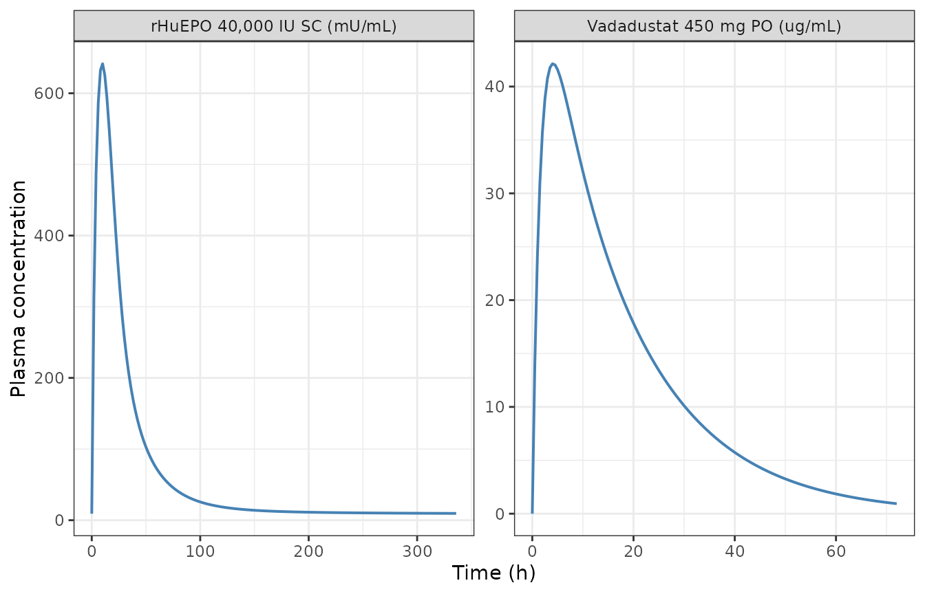
Simulated single-dose plasma profiles. Replicates Figure 2 panels A (rHuEPO, total plasma EPO activity) and C (vadadustat).
The vadadustat profile (Cmax ~40 ug/mL at 2-4 h) matches the exposure Chavan 2021 reports for a single 450 mg dose. The darbepoetin and daprodustat sub-models under-predict their published peaks; see Errata.
7. Feedback-loop behaviour (Supplementary Figure S1)
Supplementary Figure S1 shows the qualitative relationships that close the loop: PHD falls as Hb falls, HIF-alpha rises as PHD falls, and plasma EPO rises as HIF-alpha rises. Sweeping Hb across the physiological range reproduces the first two limbs analytically from the model’s own assignment rule.
hb_grid <- seq(5, 18, by = 0.1)
phd <- 52.5 / (1 + 100 / (5 + hb_grid^3.3))
hif <- 1.35 / (phd * 0.34)   # steady state of Eq. 3
bind_rows(
  tibble::tibble(x = hb_grid, y = phd, Panel = "Active PHD (ng/mL) vs Hb (g/dL)"),
  tibble::tibble(x = hb_grid, y = hif, Panel = "Steady-state HIF-alpha (ng/mL) vs Hb (g/dL)")
) |>
  ggplot(aes(x, y)) +
  geom_line(linewidth = 0.7, colour = "firebrick") +
  facet_wrap(~Panel, scales = "free_y") +
  labs(x = "Hemoglobin (g/dL)", y = NULL) +
  theme_bw()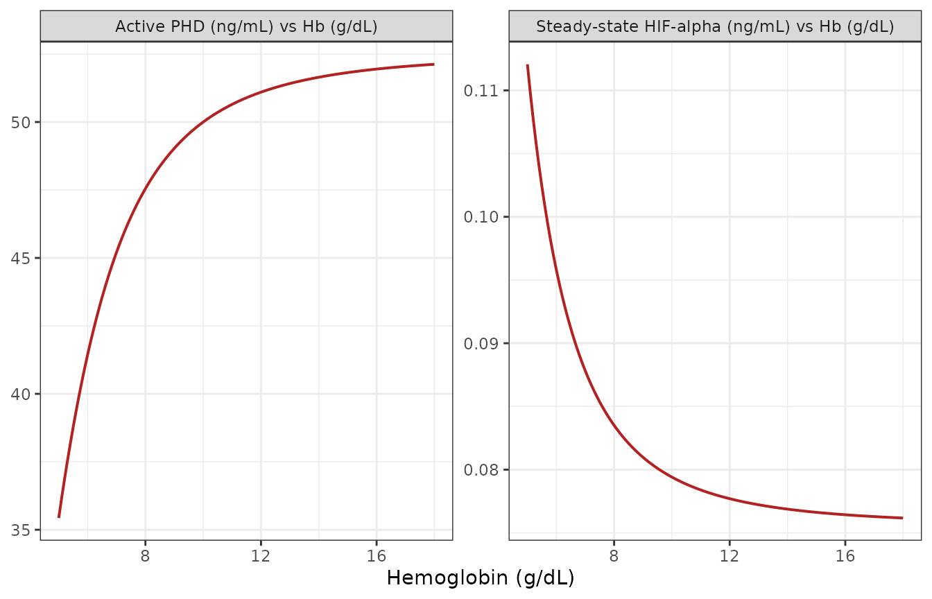
Hb-PHD and PHD-HIF limbs of the feedback loop. Replicates Supplementary Figure S1 (top left, bottom left).
Active PHD decreases and HIF-alpha increases as Hb falls, the direction required for the anemia-sensing loop to work.
Assumptions, deviations and errata
Modelling assumptions carried from the paper. Iron sufficiency is assumed (no iron, hepcidin or ferritin sub-model); EPO diurnal variability is not captured, so simulated EPO should not be interpreted on a sub-daily timescale; hemodialysis blood loss is not represented; and EPOR saturation is assumed not to occur. The model captures disease at a steady state, which limits predictions to horizons of a few months.
Single compartment for plasma and bone marrow. The Supplement notes that progenitors and precursors physically reside in bone marrow but are modelled in the central compartment, so simulated progenitor and precursor numbers are not reliable; the endpoints of the chain (plasma EPO, reticulocytes, RBC, Hb) are. That caveat carries over to this implementation.
Amplification factor 32 is not in the main text.
Equation 18 gives precursor production as
k_progenitorsToPrecursors * Progenitors, but the authors’
SimBiology reaction_29 uses
k_progenitorsToPrecursors * Progenitors * 32. The factor
represents the cell divisions between the CFU-E and reticulocyte stages.
It is load-bearing: the model file follows the released code, exposing
it as progenitorAmplification, because without it the chain
cannot reach the reported RBC and Hb levels.
Endogenous EPO off-rate is written as
kon * kd. reaction_8_1 encodes the
endogenous EPO dissociation rate as kon_EPO_LR_complex * kd
rather than using koff_EPO_LR_complex directly. With the
dashboard values these agree exactly (1e-13 * 5.5e13 = 5.5 =
koff_EPO_LR_complex), so the two ligands do share binding
kinetics as the paper states; the model file preserves the released
form.
Unit conversions made explicit. The two factors described in the units table above are implicit in the released SimBiology project (which runs with unit conversion enabled) and are written out here. Section 3 demonstrates that the receptor-binding factor is required for the model to have any pharmacodynamics at all.
Minor: the declared unit of PHI_periphery is
inconsistent. The Parameter Dashboard “Species” sheet declares
PHI_periphery in ug/mL while PHI_Plasma, and
every other peripheral species, is declared in ng/mL. Taken literally
the distribution term
CLD_PHI * (PHI_Plasma - PHI_periphery) would then subtract
two quantities a factor of 1000 apart. This implementation reads both
states as ng/mL, which is the self-consistent interpretation and the one
that reproduces the paper’s vadadustat response above; the declared
ug/mL is treated as a slip in the sheet. The state starts at zero either
way, so nothing in the steady-state results depends on the choice.
Solver guard on the PHI Hill function.
PHI_Plasma^0.17 has an infinite derivative at zero, which
stalls the integrator during the undosed equilibration run. A
1e-24 offset is added inside the power. This is a numerical
guard, not a model change, and is negligible at any dosed
concentration.
Erratum: the Healthy k_deg_prog in the Parameter
Dashboard is not usable as printed. The dashboard gives
k_deg_prog = 0.000694 1/h for the healthy virtual patient.
Simulated forward, that value produces a steady-state hemoglobin of
182 g/dL – physically impossible and about 13x the
paper’s own healthy value. Three independent lines of evidence identify
it as a transcription error and fix the value at approximately
0.0669 1/h:
- The printed value is an exact duplicate of the CKD 5
kdeg_RBCMcell (0.000694) in the same table, the signature of a copy error. - The other four stages’ printed values reproduce the paper’s reported stage-wise Hb correctly (CKD 3 12.05, CKD 4 9.61, CKD 5 9.11 g/dL against Figure 3’s ~12, ~10 and <10), so the surrounding transcription and the model reconstruction are sound; only the healthy cell is wrong.
- Back-solving from the healthy baseline Hb of 13.5 g/dL (Cheung 2001) gives 0.0669, which then independently predicts both Cheung therapy arms (40,000 IU QW to 16.34 vs. 16.4 reported; 10,500 IU TIW to 16.52) and restores a monotone series across stages (0.0669 > 0.0525 > 0.030 > 0.026 > 0.0158).
The back-solved value is used only in this vignette’s Healthy virtual
patient. The parameterization shipped in ini() is the CKD 4
non-dialysis reference patient, every value of which is printed in the
dashboard, so no back-solved number is distributed with the model.
Erratum: the CKD 1.5 column is internally
inconsistent. Simulated with its printed values, the CKD 1.5
patient reaches a steady-state Hb of 8.66 g/dL – below CKD 5 (9.11), and
far below the near-normal value its position in the disease sequence
implies. Its printed kprod_prog (2.0e9) also breaks the
otherwise monotone production series (3.6e9, 2.1e9, 1.5e9, 1.38e9).
Either k_deg_prog or kprod_prog could be at
fault and there is no reported Hb for this stage to discriminate between
them, so no repair was attempted and CKD 1.5 is excluded from
this vignette. The paper itself states that CKD 1.5 is a
continuity construct that “is not part of any Vpop”, so nothing in the
paper’s results depends on it.
Deviation: darbepoetin and daprodustat under-reproduce the paper’s own reference-patient responses. With the dashboard parameters, darbepoetin 55 ug Q2W raises reference-patient Hb by 1.01 g/dL against the 2.6 g/dL the Supplement reports, and daprodustat 4 mg QD gives 1.93 against 1.4. Both discrepancies originate in the drug-specific PK sub-models rather than in the shared erythropoiesis core: simulated darbepoetin Cmax after 60 ug SC is 2.45 ng/mL at 20 h against the roughly 5-8 ng/mL at 48-72 h that Kim 2019 reports, and simulated daprodustat Cmax after 4 mg is 63 ng/mL against the 100-300 ng/mL range of Yamada 2020. Since the same core reproduces rHuEPO and vadadustat to within 5%, the most likely explanation is an incompletely transcribed darbepoetin/daprodustat PK parameter set in the dashboard. No parameter was tuned to close these gaps; the dashboard values are shipped as published and the discrepancy is reported here.
No IIV or residual error. The paper reports neither, so the model file contains neither. Virtual populations in the paper are built by log-normal resampling of the sensitive parameters listed in Supplementary Table S2 around a reference patient, followed by filtering on baseline Hb; that workflow is a property of the authors’ MATLAB scripts, not of the model, and is not reproduced here.
Adaptive dose titration not implemented. The paper’s population results (Figures 5-9) depend on per-patient adaptive dose-titration algorithms applied during simulation. Those are trial-protocol logic rather than model structure and are outside the scope of a model file; the fixed-dose reference-patient responses validated above are the model-level equivalent.