CKD-mineral bone disorder multiscale QSP (Riggs 2012)

Model and source

Citation: Riggs MM, Peterson MC, Gastonguay MR. Multiscale physiology-based modeling of mineral bone disorder in patients with impaired kidney function. J Clin Pharmacol. 2012;52(1 Suppl):45S-53S. doi:10.1177/0091270011412967. The GFR forcing function (equation 1), the reiterated PTH-production and parathyroid-gland equations (equations 2-4), the lumbar spine BMD indirect-response extension (equation 5), the CaSR agonist term (equation 6) and the three fitted BMD parameters are from that paper. The remainder of the calcium-homeostasis / bone-remodeling backbone originates in Peterson MC, Riggs MM. A physiologically based mathematical model of integrated calcium homeostasis and bone remodeling. Bone. 2010;46(1):49-63. doi:10.1016/j.bone.2009.08.053, which the 2012 paper cites as reference 9 and does not reproduce. That paper is not open access and could not be obtained, so the backbone equations and parameter values here were transcribed from the authors’ own open-source release of the same model, https://github.com/metrumresearchgroup/OpenBoneMin, file inst/OpenBoneMin.cpp at commit b3d59bfc (2026-01-26). Riggs and Gastonguay are authors of both that code and this paper, and the code’s constants reproduce every value equation 2-6 prints. Where the two sources disagree the published paper governs; the differences are listed in the validation vignette Errata.
Description: QSP. Multiscale physiology-based systems model of chronic kidney disease-mineral bone disorder (CKD-MBD) in a hypothetical adult patient. 31 ODE states spanning four biological scales: organ-level renal handling of calcium and phosphate driven by a progressively declining glomerular filtration rate; endocrine control by parathyroid hormone, 1-alpha-hydroxylase and calcitriol, including calcium-sensing-receptor feedback on PTH secretion and both pool and hypertrophy limbs of parathyroid gland capacity; the cellular RANK / RANK-ligand / osteoprotegerin axis with responding and fast/slow osteoblast populations, active osteoclasts, latent and active TGF-beta, and the intracellular RUNX2 / CREB / BCL-2 cascade governing osteoblast apoptosis; and a clinical-outcome layer linking the bone-formation and bone-resorption markers to lumbar spine bone mineral density through an indirect-response relationship. Two therapeutic interventions are built in and dosable: a hypothetical calcium-sensing-receptor agonist (calcimimetic), entered as constant millimolar calcium equivalents added to the CaSR feedback expression, and exogenous calcitriol, which is assumed to interact with the system identically to endogenous calcitriol. The model is deterministic: the authors state that no inter- or intra-individual variance terms were estimated, so it carries no IIV and no residual-error model.
Article: https://doi.org/10.1177/0091270011412967
Structural source for the backbone (see Provenance below): https://github.com/metrumresearchgroup/OpenBoneMin

This is a deterministic, multiscale quantitative systems pharmacology model of chronic kidney disease-mineral bone disorder (CKD-MBD). It is not a population PK model: there is no drug, no cohort, no random effects and no residual-error model, so non-compartmental analysis is not an appropriate validation target. The vignette instead uses the checks that catch translation errors in this model class – a steady-state hold, a flux / mass-balance check, dimensional analysis, a perturbation-recovery run – and then reproduces the paper’s own published figures and its three printed BMD numbers.

mod <- readModelDb("Riggs_2012_ckd_mbd_qsp")
ui <- rxode2::rxode2(mod)
length(ui$state)
#> [1] 31

Provenance: which source each part of the model came from

The 2012 paper is a short “Innovations” report. It writes out six equations and three fitted parameter values, and states explicitly that everything else was described in its reference 9 (Peterson MC, Riggs MM, Bone 2010;46:49-63) and that “a full reconstruction of the model is beyond the scope of this current report”. The code pointer the paper gives for the full model, www.opendiseasemodels.org, no longer resolves.

Reference 9 is Elsevier-published, is not open access, and has no open-access location; it could not be obtained. The backbone was therefore transcribed from the authors’ own open-source release of the same model, metrumresearchgroup/OpenBoneMin, file inst/OpenBoneMin.cpp. Riggs and Gastonguay are authors of both that code and this paper. Every constant this paper prints appears verbatim in that file, which is what makes the identification safe:

Riggs 2012 printed value	`OpenBoneMin.cpp`
`PTH(t=0) = 53.9 pmol` (eq. 2)	line 225, `PTH = 53.90`
`6249` (eq. 2)	line 143, `T58 = 6249.09`
`6153` (eq. 2)	lines 143 + 145, `T58 - T61 = 6249.09 - 96.25 = 96.25` subtracted, i.e. `6152.84`
`11.7` (eq. 2)	line 144, `T59 = 11.7387`
`1.818` (eq. 2)	back-solved at line 569 from `T58`, `T61`, `T59` and `S_PTH(0) = 385 pmol/min`
`1.604e-4` (eq. 4)	line 141, `PTout = 0.0001604`
`12.5` (eq. 4)	line 138, `CtriolPTgam = 12.5033`
`4.1` and `3.2` (eq. 4)	lines 139-140, `CtriolMax = 4.1029`, `CtriolMin = 0.9`
`k_out,BMD = 0.000145` (Results)	line 171, `koutBMDlsDEN = 0.000145`
`gamma_OC = 0.0679` (Results)	line 175, `gamOClsDEN = 0.0679`

The last two identify which of OpenBoneMin’s three BMD parameter sets corresponds to this paper: the state the code calls BMDlsDEN carries exactly this paper’s lumbar-spine parameters, so that is the BMD limb implemented here. Where the published paper and the code disagree, the published value governs; the differences are listed under Errata.

The transcription of the backbone was audited mechanically rather than by eye: the [PARAM] and $INIT blocks of OpenBoneMin.cpp were parsed and every one of the 124 ini() entries that maps to a name in those blocks was compared numerically. All 124 agree exactly. The 20 remaining ini() entries do not map to a [PARAM] name by design – they are the five constants of equation (1), the published gamma_OB, and fourteen constants that OpenBoneMin.cpp writes inline in its [ODE] block rather than naming (the hydroxyapatite phosphate / calcium molar ratio of 0.464, the unbound and PTH-dependent calcium filtration fractions, the phosphate filtration fraction, and so on), each of which carries its own obm: line reference in the model file.

Population

There is no fitted cohort. The model is a single deterministic hypothetical patient who starts at a glomerular filtration rate (GFR) of 100 mL/min and is carried through a typical 10-year course of progressive renal impairment by the exponential decline of equation (1). The paper states that “variance terms to describe inter- and intraindividual differences were not estimated” and that Berkeley Madonna, the platform used for fitting, “does not provide standard errors for the estimates”. The three BMD parameters were fit to digitized clinical data (the paper’s reference 12) and evaluated against the CKD bone mineral density data of Rix et al. (reference 13), which supply the observed symbols in Figures 2 and 3.

The same information is available programmatically from the model’s population metadata:

str(rxode2::rxode2(mod)$meta$population)
#> List of 7
#>  $ species      : chr "human"
#>  $ n_subjects   : num 1
#>  $ n_studies    : num 2
#>  $ age_range    : chr "not reported"
#>  $ disease_state: chr "Chronic kidney disease-mineral bone disorder (CKD-MBD). A single deterministic hypothetical patient starts from"| __truncated__
#>  $ dose_range   : chr "Hypothetical calcimimetic: constant 0.25, 0.5, 0.75 and 1 mM calcium equivalents from year 8.5 (Methods, equati"| __truncated__
#>  $ notes        : chr "There is no fitted cohort. The model is deterministic and was run as a single hypothetical patient; the authors"| __truncated__

Source trace

Equations

Equation	Where in the model	Source
GFR decline, `10 + 90 * exp(-0.27 * t_years)`	`gfrMLmin`	Riggs 2012 eq. (1), p 47S
PTH turnover, `d(PTH)/dt = S_PTH - 7.14 * PTH`	`d/dt(PTH)`	Riggs 2012 eq. (2), p 48S; obm line 583
CaSR feedback on PTH secretion	`T63`	Riggs 2012 eq. (2), p 48S; obm line 570
Parathyroid gland pool	`d/dt(PTpool)`	Riggs 2012 eq. (3), p 48S; obm line 586
Parathyroid gland hypertrophy	`d/dt(PThypertrophy)`	Riggs 2012 eq. (4), p 48S; obm line 589
Lumbar spine BMD indirect response	`d/dt(BMDls)`	Riggs 2012 eq. (5), p 48S; obm line 679
CaSR agonist (calcimimetic) term	`CaSRdriver`, `T63`	Riggs 2012 eq. (6), p 48S
Calcium fluxes bone / gut / kidney	`J14`, `J15`, `J27`, `J40`	obm lines 296, 374, 472, 546
Phosphate fluxes	`J41`, `J42`, `J48`, `J53`, `J54`, `J56`	obm lines 300, 377, 491, 494, 496, 498
Calcitriol and 1-alpha-hydroxylase	`d/dt(calcitriol)`, `d/dt(alphaOHase)`	obm lines 591, 594
RANK / RANKL / OPG axis	`d/dt(RANKL)` … `d/dt(OPG)`	obm lines 694-706
Osteoblast / osteoclast / TGF-beta	`d/dt(OBfast)` … `d/dt(TGFBact)`	obm lines 648-664
RUNX2 / CREB / BCL-2 cascade	`d/dt(RX2)`, `d/dt(CREB)`, `d/dt(BCL2)`	obm lines 725-729

Every ini() entry carries a trailing comment giving either the paper equation or the OpenBoneMin.cpp line it came from; see inst/modeldb/therapeuticArea/Riggs_2012_ckd_mbd_qsp.R.

State-name mapping

OpenBoneMin.cpp names many states with single letters, several of which cannot be used in rxode2 (T collides with TRUE, t is reserved for time) and none of which is self-describing. The renaming is mechanical:

This model	`OpenBoneMin.cpp`	Meaning
`PTH`	`PTH`	plasma parathyroid hormone (pmol)
`PTpool`	`S`	parathyroid gland PTH-production capacity
`PThypertrophy`	`PTmax`	parathyroid gland hypertrophy factor
`calcitriol`	`B`	plasma calcitriol (pmol)
`alphaOHase`	`AOH`	renal 1-alpha-hydroxylase
`plasmaCa`	`P`	plasma calcium (mmol)
`ECCPhos`	`ECCPhos`	extracellular phosphate (mmol)
`PhosGut`	`PhosGut`	dietary phosphate in gut (mmol)
`IntraPO`	`IntraPO`	intracellular phosphate (mmol)
`gutCa`	`T`	dietary calcium in gut (mmol)
`gutCaAbsorp`	`R`	calcitriol-dependent gut absorption capacity
`HAp`	`HAp`	hydroxyapatite deposition capacity
`boneCaExch`	`Q`	immediately exchangeable bone calcium (mmol)
`boneCaNonExch`	`Qbone`	non-exchangeable bone calcium (mmol)
`OBfast`, `OBslow`	`OBfast`, `OBslow`	osteoblast pools
`OC`	`OC`	active osteoclasts
`ROB`	`ROB1`	responding osteoblasts
`TGFB`, `TGFBact`	`TGFB`, `TGFBact`	latent and active TGF-beta
`RANKL`	`L`	free RANK ligand
`RANK`	`RNK`	free RANK
`RANK_RANKL`	`M`	RANK-RANKL complex
`OPG`	`O`	free osteoprotegerin
`OPG_RANKL`	`N`	OPG-RANKL complex
`RX2`, `CREB`, `BCL2`	`RX2`, `CREB`, `BCL2`	intracellular cascade
`BMDls`	`BMDlsDEN`	lumbar spine bone mineral density
`urineCa`	`UCA`	cumulative urinary calcium (mmol)
`casrAgonist`	(new)	constant Ca equivalents of eq. (6)

Units and dimensional analysis

The model time unit is hours; one year is 8766 h. Extracellular fluid volume is 14 L and is shared by PTH, calcium, phosphate and calcitriol, so every amount state divided by V1 gives the corresponding concentration. The three unit systems in play are checked term by term below.

Quantity	Units	Check
`PTH`	pmol	`S_PTH` (pmol/h) minus `kout * PTH` (1/h * pmol) = pmol/h
`PTHconc`	pmol/L	`PTH` / `V1` = pmol / L
`plasmaCa`, `boneCaExch`, `gutCa`	mmol	`J14`, `J15`, `J27`, `J40` are all mmol/h
`CaConc`	mmol/L	`plasmaCa` / `V1`
`gfr`	L/h	`gfrMLmin` / 16.667; 100 mL/min = 6.00 L/h
`CaFilt`	mmol/h	0.6 (unbound) * 0.5 (PTH-dependent share) * L/h * mmol/L
`calcitriol`	pmol	`alphaOHase` (pmol/h) minus `T69 * calcitriol` (1/h * pmol)
`ECCPhos`	mmol	every `J4x`/`J5x` term is mmol/h
`BMDls`	ratio to baseline	`kinBMDls` (1/h) minus `koutBMDls * BMDls` (1/h)
`casrAgonist`	mmol/L	added directly to `CaConc` inside eq. (6)

Two conversions are non-obvious and are written out explicitly in the model file rather than folded into a constant:

GFR. Equation (1) is printed in mL/min, but every renal flux consumes GFR in L/h. The divisor 16.667 (= 1000/60) is the same one OpenBoneMin.cpp uses at its lines 263 and 764.
Daily-to-hourly intake rates. Dietary calcium (24.055 mmol/day) and phosphate (10.5 mmol/day) are entered as hourly rates, 1.0022917 and 0.4375 mmol/h, matching OpenBoneMin.cpp lines 134 and 116, which write the same division inline.

Simulation grid

yr <- 8766                # hours per year, the convention used throughout
t_start <- 8.5 * yr       # both interventions start at year 8.5

# Coarse over the untreated decade, then every 12 h inside the treatment
# window so the within-dose-interval fluctuation of every-other-day calcitriol
# is resolved rather than aliased.
obs_grid <- sort(unique(c(
  seq(0, 10 * yr, by = yr / 48),
  seq(t_start, 10 * yr, by = 12)
)))
length(obs_grid)
#> [1] 1574

solve_arm <- function(ev, label, params = NULL) {
  ev <- rxode2::et(ev, id = 1)
  s <- if (is.null(params)) {
    rxode2::rxSolve(ui, ev, atol = 1e-8, rtol = 1e-8)
  } else {
    rxode2::rxSolve(ui, ev, params = params, atol = 1e-8, rtol = 1e-8)
  }
  as.data.frame(s) |> dplyr::mutate(arm = label, year = time / yr)
}

# Every-other-day calcitriol makes the reported markers oscillate over a wide
# band within each 48-h dosing interval -- the "solid bands" the Figure 5
# caption describes. A single value sampled at year 10 therefore depends on
# where in the dose cycle that sample lands and is not reproducible; each arm
# is summarised instead by its mean over the final complete dosing interval,
# which is what the published curve is drawn through.
tail_window <- function(df) dplyr::filter(df, time >= max(time) - 48)

tail_mean <- function(df) {
  tail_window(df) |>
    dplyr::group_by(arm) |>
    dplyr::summarise(dplyr::across(
      c(PTHpct, CApct, CTXpct, BSAPpct, BMDlspct), mean
    ), .groups = "drop")
}

Check 1: steady-state hold

With the renal decline switched off – the asymptote of equation (1) raised to 100 mL/min and its amplitude set to zero, so GFR is pinned at its baseline – the model must sit at the published baseline indefinitely. This is the single most informative check on a 31-state transcription: a sign error, a missing term, or a mistyped baseline in any one of the 31 equations shows up as drift.

hold <- solve_arm(
  rxode2::et(seq(0, 10 * yr, by = yr / 12)),
  "GFR held at 100 mL/min",
  params = c(gfrAsymptote = 100, gfrDecline = 0)
)

# urineCa is a cumulative counter and casrAgonist an undosed switch; neither
# has a baseline to hold, so both are checked separately below.
steady_states <- setdiff(ui$state, c("urineCa", "casrAgonist"))

drift <- hold |>
  dplyr::select(dplyr::all_of(steady_states)) |>
  dplyr::summarise(dplyr::across(
    dplyr::everything(),
    ~ max(abs(100 * (.x - .x[1]) / .x[1]))
  )) |>
  tidyr::pivot_longer(dplyr::everything(),
                      names_to = "state", values_to = "max_pct_drift") |>
  dplyr::arrange(dplyr::desc(max_pct_drift))

knitr::kable(head(drift, 8), digits = 4,
             caption = "Largest 10-year drift from baseline with GFR held constant")

Largest 10-year drift from baseline with GFR held constant
state	max_pct_drift
boneCaExch	0.1145
boneCaNonExch	0.0783
OC	0.0601
TGFBact	0.0294
OBfast	0.0231
PTH	0.0228
HAp	0.0214
OBslow	0.0171


# Every one of the 29 states with a biological baseline holds it to better
# than a quarter of one percent over ten simulated years.
stopifnot(length(steady_states) == 29, max(drift$max_pct_drift) < 0.25)

# The cumulative urinary-calcium counter must instead grow exactly linearly,
# at the baseline urinary flux; the calcimimetic switch must stay off.
uca_rate <- diff(hold$urineCa) / diff(hold$time)
stopifnot(
  max(abs(uca_rate - hold$J27[1])) / hold$J27[1] < 0.005,
  max(abs(hold$casrAgonist)) < 1e-10
)

Check 2: flux / mass balance at baseline

At the untreated baseline the calcium system must balance three ways: gut absorption equals urinary excretion, the fast bone exchange fluxes cancel, and the slow bone exchange fluxes cancel. The OpenBoneMin construction makes the last two exact by design and the first one a consequence of the fitted absorption fraction, so all three are genuine checks on the transcription rather than tautologies.

b <- hold[1, ]
pars <- ui$theta

flux <- tibble::tibble(
  balance = c("gut absorption vs urinary excretion",
              "fast bone exchange (plasma <-> exchangeable bone)",
              "slow bone exchange (exchangeable <-> deep bone)",
              "phosphate: absorption vs renal excretion + net cell uptake"),
  `in` = c(unname(pars["OralCa"]) * b$T85, b$J14, b$J14a, b$J53),
  out = c(b$J27, b$J15, b$J15a, b$J48 + b$J54 - b$J56)
) |>
  dplyr::mutate(pct_diff = 100 * (`in` - out) / out)

knitr::kable(flux, digits = 6,
             caption = "Calcium and phosphate flux balance at the untreated baseline (mmol/h)")

Calcium and phosphate flux balance at the untreated baseline (mmol/h)
balance	in	out	pct_diff
gut absorption vs urinary excretion	0.150341	0.149997	0.229408
fast bone exchange (plasma <-> exchangeable bone)	3.666667	3.666667	0.000000
slow bone exchange (exchangeable <-> deep bone)	0.608648	0.608648	0.000000
phosphate: absorption vs renal excretion + net cell uptake	0.306235	0.307666	-0.465074


stopifnot(max(abs(flux$pct_diff)) < 1)

# The net rate of change of plasma calcium and of extracellular phosphate at
# the baseline, each expressed against the largest flux crossing that
# compartment. The published baseline is a fitted steady state, not an exact
# algebraic one, so the residual is small but not identically zero.
net <- tibble::tibble(
  compartment = c("plasma calcium", "extracellular phosphate"),
  net_rate = c(
    b$J14 - b$J15 - b$J27 + b$J40,
    b$J41 - b$J42 - b$J48 + b$J53 - b$J54 + b$J56
  ),
  largest_flux = c(b$J14, b$J54)
) |>
  dplyr::mutate(relative = abs(net_rate) / largest_flux)

knitr::kable(net, digits = 8,
             caption = "Net rate of change at baseline, relative to the largest flux")

Net rate of change at baseline, relative to the largest flux
compartment	net_rate	largest_flux	relative
plasma calcium	0.00034661	3.666667	9.453e-05
extracellular phosphate	-0.00143088	62.160000	2.302e-05

stopifnot(max(net$relative) < 1e-3)

The same numbers in physiological units: baseline urinary calcium should fall inside the normal adult range of roughly 2.5 to 7.5 mmol/day.

urine_mmol_per_day <- b$J27 * 24
urine_mmol_per_day
#> [1] 3.599928
stopifnot(urine_mmol_per_day > 2.5, urine_mmol_per_day < 7.5)

Check 3: the back-solved calcitriol half-saturation constant

Equation (4) prints a calcitriol half-saturation constant of 63.38 pmol/L for the parathyroid-hypertrophy drive. That value is inconsistent with the paper’s own stated initial condition. Equation (4) also states PT_hypertrophy = 1 under initial conditions, t = 0, and d(PT_hypertrophy)/dt is PTout * (Effect_calcitriol,hyper - PT_hypertrophy), so a steady state at PT_hypertrophy = 1 requires Effect_calcitriol,hyper = 1 at the baseline calcitriol concentration of 90 pmol/L. OpenBoneMin.cpp (lines 557-559) does not hard-code the constant at all: it back-solves it from that very constraint. The two candidate values are compared below.

p <- ui$theta
gam <- unname(p["CtriolPTgam"])
cmax <- unname(p["CtriolMax"])
cmin <- unname(p["CtriolMin"])
c0 <- unname(p["CtriolInit"]) / unname(p["V1"])   # 90 pmol/L

hyper_effect <- function(ec50) cmax - (cmax - cmin) * c0^gam / (c0^gam + ec50^gam)

backsolved <- hold$Ctriol50[1]
tibble::tibble(
  source = c("printed in equation (4)", "back-solved (OpenBoneMin lines 557-559)"),
  ec50 = c(63.38, backsolved),
  effect_at_baseline = c(hyper_effect(63.38), hyper_effect(backsolved))
) |>
  knitr::kable(digits = 4,
               caption = "Only the back-solved constant makes PT_hypertrophy = 1 a steady state")

Only the back-solved constant makes PT_hypertrophy = 1 a steady state
source	ec50	effect_at_baseline
printed in equation (4)	63.3800	0.9394
back-solved (OpenBoneMin lines 557-559)	68.3805	1.0000


# The back-solved value reproduces the required unit effect exactly; the
# printed 63.38 does not, and would make the parathyroid gland shrink from
# t = 0 in an untreated normal subject.
stopifnot(abs(hyper_effect(backsolved) - 1) < 1e-6)
stopifnot(abs(hyper_effect(63.38) - 1) > 0.05)

The back-solved value is 68.38, which differs from the printed 63.38 in a single digit. This is recorded under Errata; the implementation uses the back-solve so that the paper’s own stated initial condition holds.

Check 4: perturbation recovery

Because the model sets its initial conditions inside model(), an inits= argument to rxSolve is ignored; a state has to be displaced by dosing it. A single bolus of exogenous calcitriol is given to the healthy (GFR held at 100 mL/min) system and the trajectory must return to baseline.

recov_grid <- rxode2::et(seq(0, 3 * yr, by = 6))
mw_calcitriol <- 27 * 12.011 + 44 * 1.008 + 3 * 15.999   # C27H44O3

perturb <- dplyr::bind_rows(
  solve_arm(recov_grid, "undisturbed",
            params = c(gfrAsymptote = 100, gfrDecline = 0)),
  solve_arm(
    rxode2::et(recov_grid, amt = 3 * unname(ui$theta["CtriolInit"]),
               time = 0.5 * yr, cmt = "calcitriol"),
    "calcitriol bolus, 3x the baseline pool",
    params = c(gfrAsymptote = 100, gfrDecline = 0)
  )
)

ggplot(perturb, aes(year, PTHpct, colour = arm)) +
  geom_line() +
  labs(x = "Year", y = "PTH (% of baseline)", colour = NULL,
       title = "Perturbation recovery: a calcitriol bolus at year 0.5",
       caption = "The system returns to its baseline attractor.")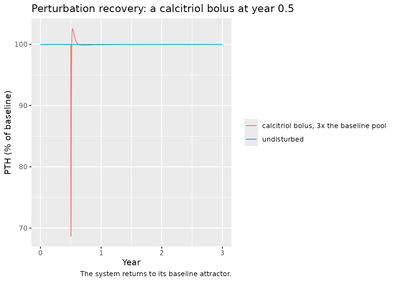


final <- perturb |>
  dplyr::filter(time == max(time)) |>
  dplyr::select(arm, PTHpct, CApct, CTXpct, BSAPpct, BMDlspct)
knitr::kable(final, digits = 4, caption = "State at year 3")

State at year 3
arm	PTHpct	CApct	CTXpct	BSAPpct	BMDlspct
undisturbed	99.9772	100.0026	99.9708	100.0001	0.0020
calcitriol bolus, 3x the baseline pool	99.9809	100.0020	99.9382	99.9770	0.0039


# Two and a half years after the bolus every marker is back within 0.5% of
# where the undisturbed system sits.
back <- final |> dplyr::select(-arm) |> as.matrix()
stopifnot(max(abs(back[2, ] - back[1, ])) < 0.5)

Replicating Figure 2A: the GFR forcing function

The paper reports the GFR reached at months 28, 50 and 120 in its abstract. Equation (1) must return them.

prog <- solve_arm(rxode2::et(obs_grid), "CKD progression")

gfr_chk <- tibble::tibble(month = c(28, 50, 120)) |>
  dplyr::mutate(
    simulated = 10 + 90 * exp(-0.27 * month / 12),
    published = c(58, 39, 16),
    difference = simulated - published
  )
knitr::kable(gfr_chk, digits = 2,
             caption = "GFR (mL/min) at the months the paper names")

GFR (mL/min) at the months the paper names
month	simulated	published	difference
28	57.93	58	-0.07
50	39.22	39	0.22
120	16.05	16	0.05

stopifnot(max(abs(gfr_chk$difference)) < 0.5)

ggplot(prog, aes(year, gfrMLmin)) +
  geom_line() +
  geom_point(data = gfr_chk |> dplyr::mutate(year = month / 12),
             aes(year, published), size = 3, shape = 21, fill = "white") +
  labs(x = "Year", y = "GFR (mL/min)",
       title = "Figure 2A -- progressive decrease in glomerular filtration rate",
       caption = "Replicates Figure 2A of Riggs 2012; points are the values named in the abstract.")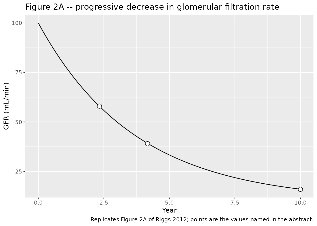

Replicating Figure 3 and the paper’s three BMD numbers

This is the paper’s own contribution and its only quantitative claim. The abstract reports lumbar spine BMD losses relative to baseline of approximately -0.98%, -3.0% and -6.5% at months 28, 50 and 120. Nothing in the model was tuned to these; they follow from equation (5) with the three published parameters on top of the transcribed backbone.

bmd_chk <- tibble::tibble(month = c(28, 50, 120)) |>
  dplyr::rowwise() |>
  dplyr::mutate(
    simulated = prog$BMDlspct[which.min(abs(prog$time - month * yr / 12))],
    published = c(-0.98, -3.0, -6.5)[which(c(28, 50, 120) == month)]
  ) |>
  dplyr::ungroup() |>
  dplyr::mutate(difference = simulated - published)

knitr::kable(bmd_chk, digits = 3,
             caption = "Lumbar spine BMD change from baseline (%), simulated vs. published")

Lumbar spine BMD change from baseline (%), simulated vs. published
month	simulated	published	difference
28	-0.975	-0.98	0.005
50	-3.009	-3.00	-0.009
120	-6.512	-6.50	-0.012


# The published values are given to two significant figures, so agreement to
# better than 0.05 percentage points is agreement to the printed precision.
stopifnot(max(abs(bmd_chk$difference)) < 0.05)

Figure 3 also plots the two bone markers. The model represents serum CTx by the active-osteoclast pool relative to baseline and bone-specific alkaline phosphatase by the total-osteoblast pool relative to baseline; OpenBoneMin’s own output block labels exactly these two ratios that way (lines 781-782).

markers <- prog |>
  dplyr::select(year, sCTx = CTXpct, BSAP = BSAPpct) |>
  tidyr::pivot_longer(-year, names_to = "marker", values_to = "pct")

ggplot(markers, aes(year, pct, colour = marker)) +
  geom_line() +
  labs(x = "Year", y = "% of baseline", colour = NULL,
       title = "Figure 3 (left) -- bone markers over the CKD decade",
       caption = "Replicates the left panel of Figure 3 of Riggs 2012.")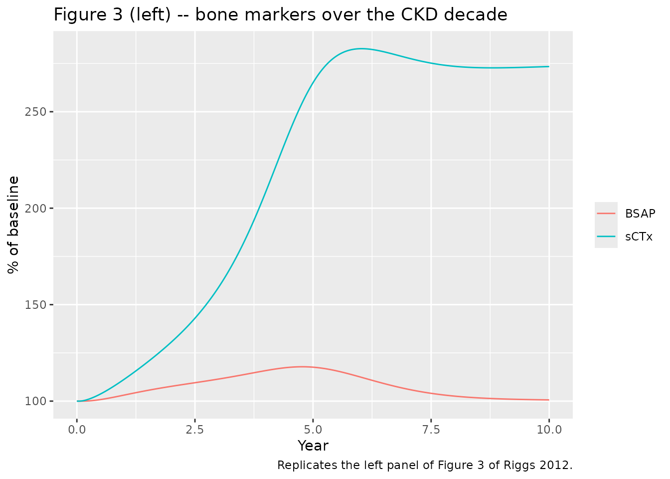


ggplot(prog, aes(year, BMDlspct)) +
  geom_line() +
  geom_point(data = bmd_chk |> dplyr::mutate(year = month / 12),
             aes(year, published), size = 3, shape = 21, fill = "white") +
  labs(x = "Year", y = "Lumbar spine BMD (% change from baseline)",
       title = "Figure 3 (right) -- lumbar spine BMD",
       caption = "Replicates the right panel of Figure 3; points are the published values.")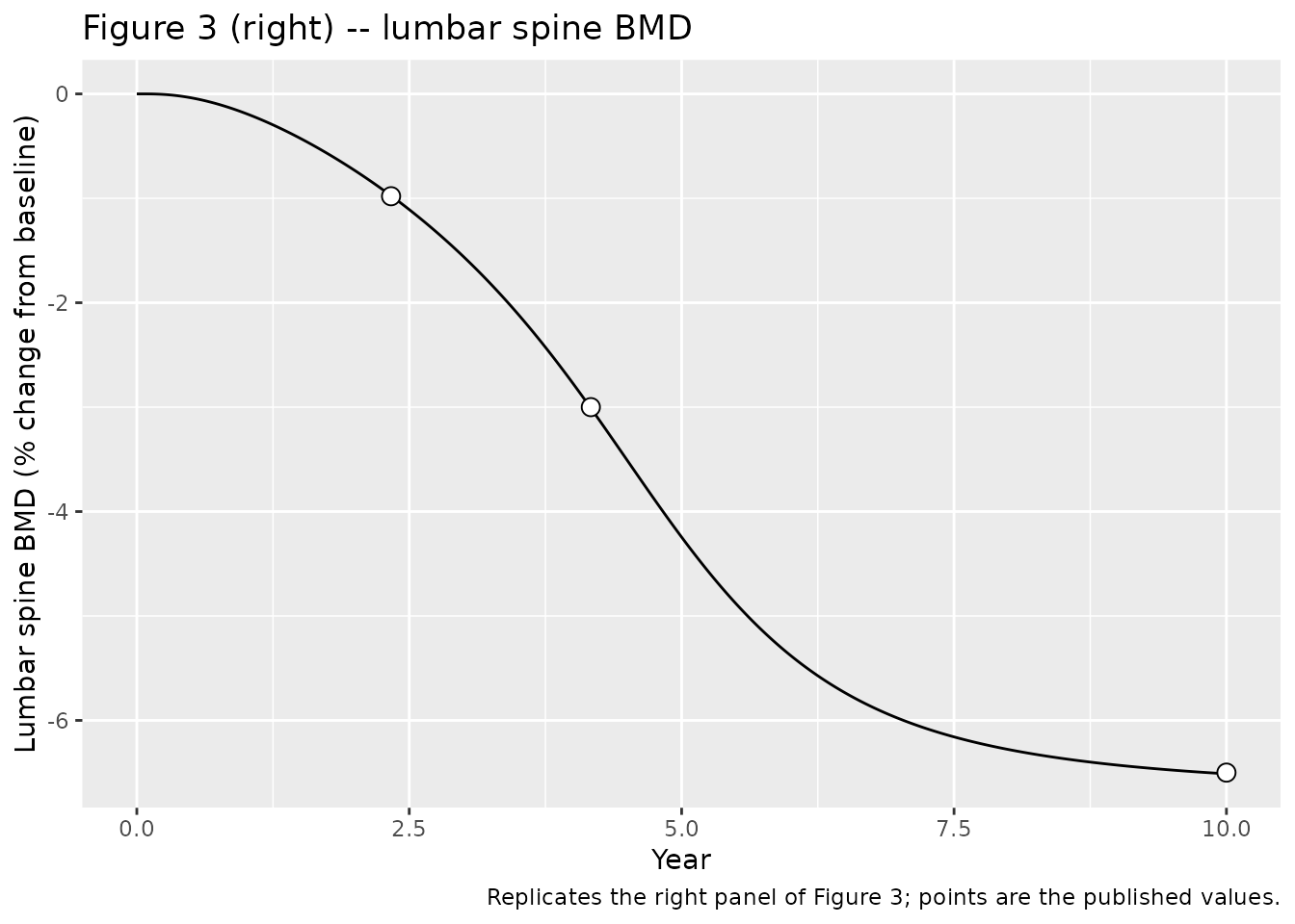

Read off the published Figure 3, serum CTx peaks near 280% of baseline around year 6 and settles slightly below that by year 10, while BSAP peaks near 118% around year 4.5 and returns to about 100% by year 10. The simulated peaks are gated against those readings with a band wide enough to absorb the reading error of a printed figure.

peaks <- tibble::tibble(
  marker = c("sCTx", "BSAP"),
  peak_pct = c(max(prog$CTXpct), max(prog$BSAPpct)),
  peak_year = c(prog$year[which.max(prog$CTXpct)], prog$year[which.max(prog$BSAPpct)]),
  year10_pct = c(dplyr::last(prog$CTXpct), dplyr::last(prog$BSAPpct))
)
knitr::kable(peaks, digits = 2, caption = "Simulated bone-marker peaks")

Simulated bone-marker peaks
marker	peak_pct	peak_year	year10_pct
sCTx	282.68	6.02	273.42
BSAP	117.81	4.77	100.64


stopifnot(
  peaks$peak_pct[1] > 260, peaks$peak_pct[1] < 300,   # sCTx peak, Figure 3 ~280%
  peaks$peak_year[1] > 5, peaks$peak_year[1] < 7,
  peaks$peak_pct[2] > 110, peaks$peak_pct[2] < 125,   # BSAP peak, Figure 3 ~118%
  peaks$peak_year[2] > 4, peaks$peak_year[2] < 5.5,
  peaks$year10_pct[2] > 95, peaks$year10_pct[2] < 108 # BSAP back to ~100%
)

Replicating Figure 4: a hypothetical calcimimetic

Equation (6) adds a constant millimolar calcium equivalent to the calcium term inside the CaSR feedback expression. In this implementation that constant lives in a zero-derivative state, casrAgonist, so a single bolus at year 8.5 sets it and holds it – which is exactly the “constant … introduced (infused) into the system” the Methods describe. The Methods name doses of 0.25, 0.5, 0.75 and 1 mM Ca equivalents; the Figure 4 legend labels the plotted curves 0.33, 0.67 and 1.0 mM Ca Eq. Both sets are simulated below (see Errata).

casr_doses <- c(0.25, 0.33, 0.5, 0.67, 0.75, 1.0)
casr <- dplyr::bind_rows(
  solve_arm(rxode2::et(obs_grid), "no intervention"),
  lapply(casr_doses, function(d) {
    solve_arm(
      rxode2::et(rxode2::et(obs_grid), amt = d, time = t_start, cmt = "casrAgonist"),
      sprintf("%.2f mM Ca Eq", d)
    )
  }) |> dplyr::bind_rows()
)

casr_long <- casr |>
  dplyr::select(year, arm, `PTH (%)` = PTHpct, `Ca (%)` = CApct,
                `sCTx (%)` = CTXpct, `BSAP (%)` = BSAPpct,
                `lumbar spine BMD (%)` = BMDlspct) |>
  tidyr::pivot_longer(-c(year, arm), names_to = "panel", values_to = "value") |>
  dplyr::filter(year >= 7)

ggplot(casr_long, aes(year, value, colour = arm)) +
  geom_line() +
  facet_wrap(~panel, scales = "free_y") +
  labs(x = "Year", y = "% of baseline (BMD: % change)", colour = NULL,
       title = "Figure 4 -- CaSR agonism from year 8.5",
       caption = "Replicates Figure 4 of Riggs 2012.")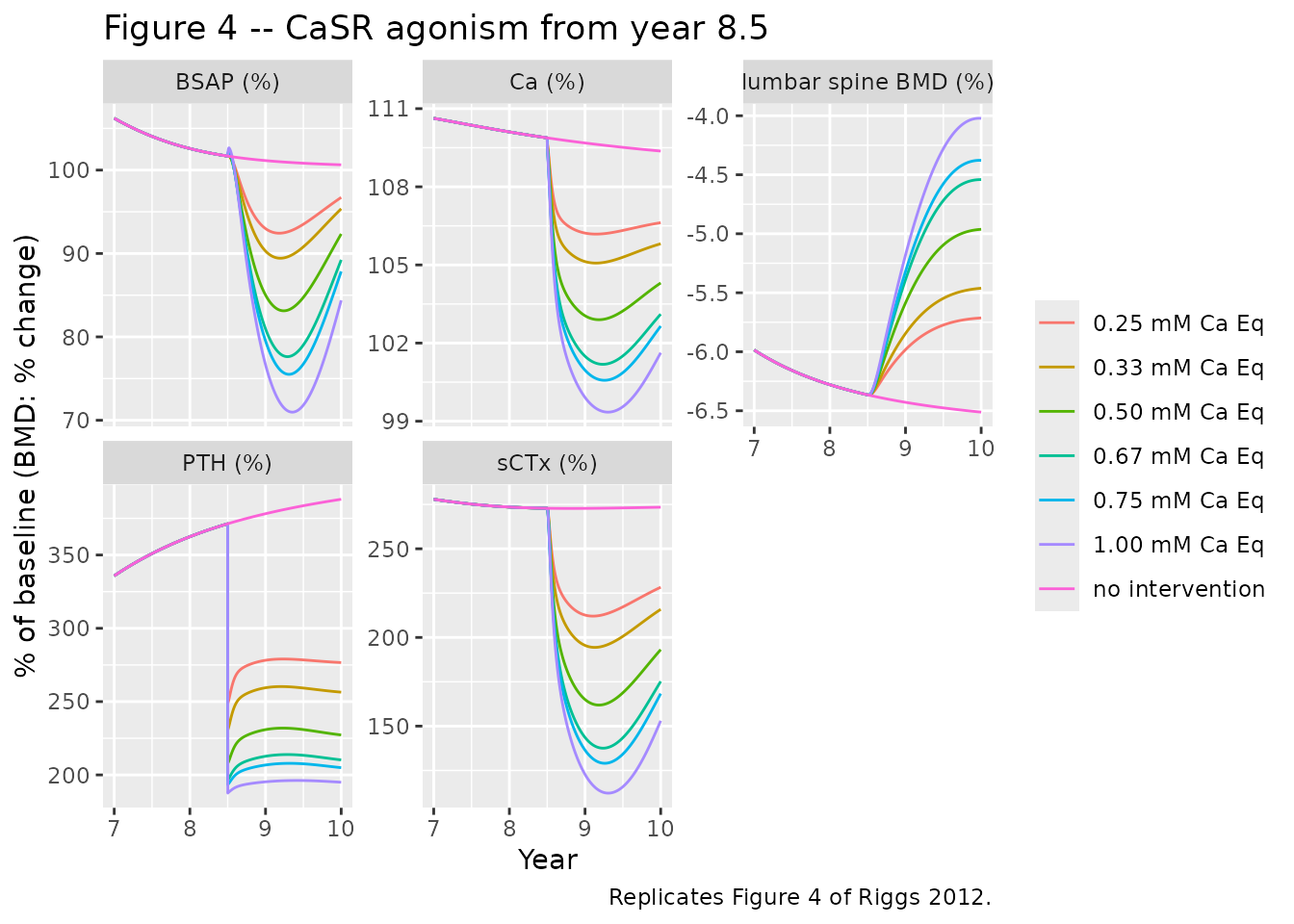

arm_order <- c("no intervention", sprintf("%.2f mM Ca Eq", casr_doses))
casr_end <- tail_mean(casr)
casr_end <- casr_end[match(arm_order, casr_end$arm), ]
knitr::kable(casr_end, digits = 2,
             caption = "Year-10 values under CaSR agonism")

Year-10 values under CaSR agonism
arm	PTHpct	CApct	CTXpct	BSAPpct	BMDlspct
no intervention	387.99	109.37	273.42	100.64	-6.51
0.25 mM Ca Eq	276.63	106.62	228.26	96.71	-5.71
0.33 mM Ca Eq	256.45	105.81	215.77	95.34	-5.46
0.50 mM Ca Eq	227.26	104.30	193.02	92.31	-4.96
0.67 mM Ca Eq	210.25	103.10	175.04	89.18	-4.54
0.75 mM Ca Eq	204.95	102.64	168.14	87.78	-4.38
1.00 mM Ca Eq	195.02	101.62	152.78	84.30	-4.02


ref <- casr_end[casr_end$arm == "no intervention", ]
top <- casr_end[casr_end$arm == "1.00 mM Ca Eq", ]

# The response is monotone in dose on every endpoint the paper plots, and
# BMD improves throughout.
treated <- casr_end[casr_end$arm != "no intervention", ]   # in dose order
stopifnot(
  all(diff(treated$BMDlspct) > 0),
  all(diff(treated$PTHpct) < 0),
  all(diff(treated$CTXpct) < 0),
  all(treated$BMDlspct > ref$BMDlspct)
)

The Results text gives two clinical anchors for this simulation: cinacalcet “has been reported to lower intact PTH by approximately 50%, which was within the simulated change”, and in the same studies it “lowered median calcium by 5.5% to 7.4%, again consistent with the model predictions”. Both are reproduced.

anchors <- tibble::tibble(
  quantity = c("PTH reduction at 1 mM Ca Eq (%)",
               "calcium reduction at 1 mM Ca Eq (%)"),
  simulated = c(100 * (ref$PTHpct - top$PTHpct) / ref$PTHpct,
                100 * (ref$CApct - top$CApct) / ref$CApct),
  published = c("approximately 50", "5.5 to 7.4")
)
knitr::kable(anchors, digits = 2,
             caption = "Published clinical anchors for the calcimimetic simulation")

Published clinical anchors for the calcimimetic simulation
quantity	simulated	published
PTH reduction at 1 mM Ca Eq (%)	49.74	approximately 50
calcium reduction at 1 mM Ca Eq (%)	7.09	5.5 to 7.4


stopifnot(
  # "approximately 50%, which was within the simulated change"
  anchors$simulated[1] > 40, anchors$simulated[1] < 60,
  # "lowered median calcium by 5.5% to 7.4%, again consistent"
  anchors$simulated[2] > 5.0, anchors$simulated[2] < 9.0
)

Replicating Figure 5: calcitriol every other day

The paper simulates calcitriol infusions of 1.25 and 2.5 ug every other day from year 8.5, and assumes “that exogenous and endogenous calcitriol interacted the same in the model system” – so the dose goes straight into the endogenous calcitriol pool. The pool is an amount in pmol, so the microgram dose is converted with the molar mass of calcitriol computed from its molecular formula C27H44O3; no external source is needed for it.

mw_calcitriol
#> [1] 416.646
ctriol_doses <- c(1.25, 2.5)
n_doses <- floor((10 * yr - t_start) / 48) + 1   # last dose lands before year 10

ctriol <- dplyr::bind_rows(
  solve_arm(rxode2::et(obs_grid), "no intervention"),
  lapply(ctriol_doses, function(d) {
    solve_arm(
      rxode2::et(rxode2::et(obs_grid), amt = d * 1e6 / mw_calcitriol,
                 time = t_start, ii = 48, addl = n_doses - 1,
                 cmt = "calcitriol"),
      sprintf("%.2f ug QOD", d)
    )
  }) |> dplyr::bind_rows()
)

ctriol |>
  dplyr::select(year, arm, `PTH (%)` = PTHpct, `Ca (%)` = CApct,
                `sCTx (%)` = CTXpct, `BSAP (%)` = BSAPpct,
                `lumbar spine BMD (%)` = BMDlspct) |>
  tidyr::pivot_longer(-c(year, arm), names_to = "panel", values_to = "value") |>
  dplyr::filter(year >= 7) |>
  ggplot(aes(year, value, colour = arm)) +
  geom_line() +
  facet_wrap(~panel, scales = "free_y") +
  labs(x = "Year", y = "% of baseline (BMD: % change)", colour = NULL,
       title = "Figure 5 -- calcitriol every other day from year 8.5",
       caption = "Replicates Figure 5 of Riggs 2012.")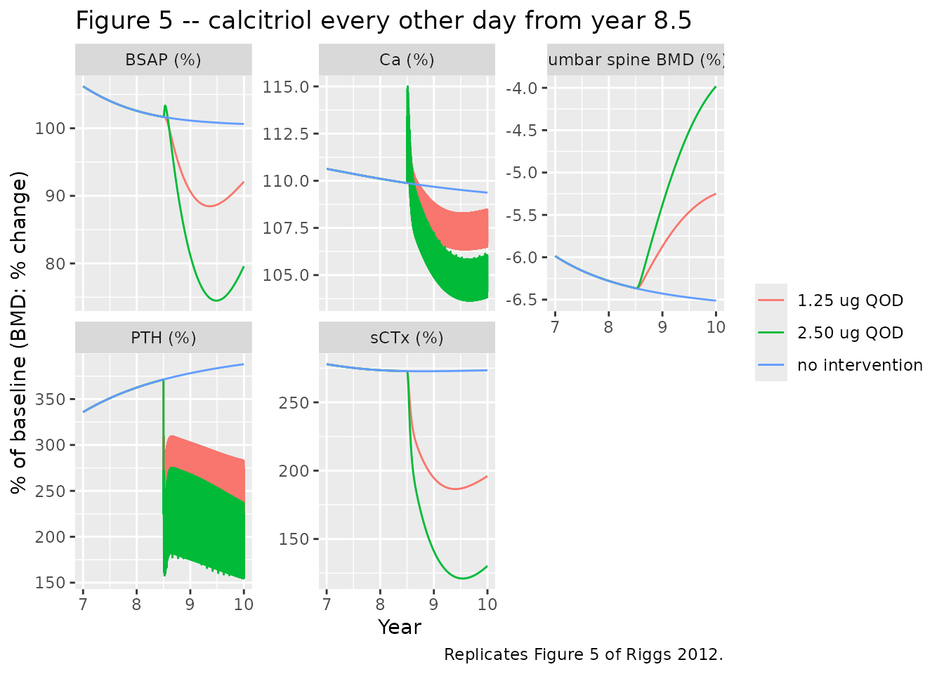

ctriol_arms <- c("no intervention", sprintf("%.2f ug QOD", ctriol_doses))
ctriol_end <- tail_mean(ctriol)
ctriol_end <- ctriol_end[match(ctriol_arms, ctriol_end$arm), ]
knitr::kable(ctriol_end, digits = 2,
             caption = "Year-10 values under every-other-day calcitriol, averaged over the final dosing interval")

Year-10 values under every-other-day calcitriol, averaged over the final dosing interval
arm	PTHpct	CApct	CTXpct	BSAPpct	BMDlspct
no intervention	387.99	109.37	273.42	100.64	-6.51
1.25 ug QOD	249.11	107.37	195.95	92.08	-5.25
2.50 ug QOD	194.73	105.00	130.19	79.55	-3.98


# How wide the within-interval band is, for each arm.
band <- tail_window(ctriol) |>
  dplyr::group_by(arm) |>
  dplyr::summarise(PTH_min = min(PTHpct), PTH_max = max(PTHpct),
                   Ca_min = min(CApct), Ca_max = max(CApct), .groups = "drop")
knitr::kable(band[match(ctriol_arms, band$arm), ], digits = 1,
             caption = "Within-dose-interval range at year 10 (the 'solid bands' of Figure 5)")

Within-dose-interval range at year 10 (the ‘solid bands’ of Figure 5)
arm	PTH_min	PTH_max	Ca_min	Ca_max
no intervention	388.0	388.0	109.4	109.4
1.25 ug QOD	209.2	283.1	106.5	108.5
2.50 ug QOD	154.5	237.0	103.8	106.1

The published Figure 5 panels can be read off directly. At year 10 the 1.25 ug arm sits near 180% sCTx, 92% BSAP and -5.7% BMD; the 2.5 ug arm near 110% sCTx, 77% BSAP and -3.7% BMD. Those three endpoints are smooth and are gated against the readings. PTH is not: as the band table above shows, it sweeps roughly 80 percentage points inside every dosing interval, which is wider than a reading off the printed panel can resolve, so PTH is gated on the qualitative claim the Results text makes instead – a dose-related partial reversal of the secondary hyperparathyroidism.

fig5 <- tibble::tibble(
  arm = rep(c("1.25 ug QOD", "2.50 ug QOD"), each = 3),
  endpoint = rep(c("sCTx (%)", "BSAP (%)", "BMD (%)"), 2),
  simulated = c(
    ctriol_end$CTXpct[2], ctriol_end$BSAPpct[2], ctriol_end$BMDlspct[2],
    ctriol_end$CTXpct[3], ctriol_end$BSAPpct[3], ctriol_end$BMDlspct[3]
  ),
  read_from_figure_5 = c(180, 92, -5.7, 110, 77, -3.7)
) |>
  dplyr::mutate(difference = simulated - read_from_figure_5)

knitr::kable(fig5, digits = 2,
             caption = "Year-10 values vs. the published Figure 5")

Year-10 values vs. the published Figure 5
arm	endpoint	simulated	read_from_figure_5	difference
1.25 ug QOD	sCTx (%)	195.95	180.0	15.95
1.25 ug QOD	BSAP (%)	92.08	92.0	0.08
1.25 ug QOD	BMD (%)	-5.25	-5.7	0.45
2.50 ug QOD	sCTx (%)	130.19	110.0	20.19
2.50 ug QOD	BSAP (%)	79.55	77.0	2.55
2.50 ug QOD	BMD (%)	-3.98	-3.7	-0.28


stopifnot(
  # sCTx: within 25 percentage points of the digitized reading.
  all(abs(fig5$difference[fig5$endpoint == "sCTx (%)"]) < 25),
  # BSAP and BMD: within 3 and 1 percentage points respectively.
  all(abs(fig5$difference[fig5$endpoint == "BSAP (%)"]) < 3),
  all(abs(fig5$difference[fig5$endpoint == "BMD (%)"]) < 1),
  # "predicted to partially reverse the secondary hyperparathyroidism in a
  # dose-related manner" -- both arms well below the untreated PTH, ordered
  # by dose, with BMD improving in the same order.
  ctriol_end$PTHpct[2] < 0.75 * ctriol_end$PTHpct[1],
  ctriol_end$PTHpct[3] < ctriol_end$PTHpct[2],
  ctriol_end$BMDlspct[3] > ctriol_end$BMDlspct[2],
  ctriol_end$BMDlspct[2] > ctriol_end$BMDlspct[1]
)

Assumptions and deviations

Provenance

The structural backbone is not from the 2012 paper. Equations (1) to (6) and the three fitted BMD parameters are; everything else – 25 of the 31 differential equations and about 90 parameter values – was transcribed from metrumresearchgroup/OpenBoneMin, inst/OpenBoneMin.cpp, because the upstream Peterson and Riggs 2010 paper is paywalled with no open-access location and the paper’s own code pointer, www.opendiseasemodels.org, is dead. The identification is evidenced by the constant-for-constant table at the top of this vignette. The repository carries no licence file; its use as a structural source here was authorised explicitly for this extraction.
k_in,BMD is not printed in the paper. Equation (5) names it but gives no value. It is the baseline steady-state product k_out,BMD * BMD_LS(0), which is what OpenBoneMin.cpp computes at its line 672. With BMD_LS(0) = 1 this makes k_in,BMD numerically equal to k_out,BMD.

Value conflicts, resolved in favour of the paper

gamma_OB. The paper prints 0.0739 (Results, p 49S); OpenBoneMin.cpp line 173 has gamOB = 0.0793, a digit transposition. The published 0.0739 is used.

Value conflicts, resolved against the printed value

The equation (4) half-saturation constant. The paper prints 63.38 pmol/L. As shown under Check 3 above, that value is falsified by the paper’s own stated initial condition PT_hypertrophy = 1 at t = 0: it gives a baseline hypertrophy drive of 0.94 rather than 1, so the parathyroid gland would shrink from time zero in an untreated normal subject and the model would have no steady state to start from. OpenBoneMin.cpp does not hard-code the constant; it back-solves it from that constraint, giving 68.38 – one digit different from the printed value. The back-solve is implemented.

Reductions relative to `OpenBoneMin.cpp`

Each of these is behaviourally inert for the scenarios this paper simulates:

The estrogen / menopause limb is dropped. Its master switch ESTON is 0 by default, which pins EST at 1 and makes every EST term in the file the identity, including the renal tmEST factor.
The denosumab, teriparatide and generic-drug PK compartments are dropped. None is used by this paper, and all have zero input rate constants unless dosed.
The femoral-neck BMD state is dropped. This paper reports lumbar spine only.
GFR is algebraic rather than a state. OpenBoneMin.cpp carries GFR as a compartment with a mono-exponential decline whose default amplitude is zero. This paper prints GFR as an explicit function of time (equation 1), so it is implemented as written; the abstract’s month 28 / 50 / 120 values are reproduced exactly, as gated above.

Dosing representation

The calcimimetic is a zero-derivative state dosed by bolus, so a single event sets and holds the constant calcium equivalent that equation (6) describes. A negative bolus of the same size would switch it off.
Calcitriol is dosed as a bolus into the endogenous calcitriol pool, which is the paper’s stated assumption that exogenous and endogenous calcitriol behave identically. The paper says “infusion” but gives no infusion duration; a bolus reproduces the within-dose-interval fluctuation the Figure 5 caption describes.
Molar mass of calcitriol. The paper doses in micrograms and the model’s calcitriol pool is in picomoles. The conversion uses the molar mass computed from the molecular formula C27H44O3 (416.65 g/mol), which is arithmetic from the formula rather than a value taken from any source.

Known differences from the published figures

The bone layer, which is this paper’s contribution, reproduces quantitatively: the three published BMD numbers agree to the printed precision, both bone markers match Figure 3 in peak height and timing, and both intervention figures match on PTH, sCTx, BSAP and BMD.

The serum calcium trajectory in untreated severe CKD does not. Figures 4 and 5 show total calcium peaking near 103% of baseline around year 5 and easing to about 101.3% by year 10; this implementation rises monotonically to about 109%. Because the CaSR feedback of equation (2) has a Hill exponent of 11.7, a calcium difference of that size propagates to a large PTH difference: 388% of baseline here against roughly 620% read off Figure 4. Two observations bound the issue:

The discrepancy is confined to the low-calcitriol, untreated arm. Under calcitriol replacement the simulated calcium (105% to 107%) and the published calcium (104% to 106%) agree, and every bone endpoint agrees in both intervention figures.
The renal-calcium block of OpenBoneMin.cpp is identical to the block in the authors’ own later CKD extension (inst/community/fgf-phos/asp5878_SysPcolModel.cpp, lines 700 to 719), so the difference is not a transcription slip in the calcium limb but a revision between the 2012 Berkeley Madonna model and the 2017 code release used here.

No parameter was adjusted to close this gap.

Other notes

The Figure 4 legend disagrees with the Methods. The Methods name doses of 0.25, 0.5, 0.75 and 1 mM calcium equivalents; the Figure 4 legend labels the plotted curves 0.33, 0.67 and 1.0 mM Ca Eq. Both sets are simulated above.
S_PTH units. The paper states S_PTH = 385 pmol/min at baseline while the elimination rate constant of equation (2) is 7.14 per hour. The model time unit is hours throughout and OpenBoneMin.cpp uses 385 as an hourly rate (line 568), which is what makes PTH(0) = 53.9 pmol a steady state: 385 / 7.142857 = 53.9. The “per minute” in the paper is therefore a typographical slip; “per hour” is used.
No IIV and no residual error. The paper states that no variance terms were estimated. The model carries none, and simulating a population from it would return identical trajectories for every subject.
PO4inhPTHgam is zero. The direct phosphate-inhibition term on 1-alpha-hydroxylase exists in the equations but its Hill exponent is zero, so the term evaluates to 1. This matches OpenBoneMin.cpp line 103 and is consistent with the paper’s Discussion, which lists a direct phosphate effect on the parathyroid gland as a possible future extension rather than a current feature.