COVID-19 pathophysiology and treatment QSP model (Rao 2023)
Source:vignettes/articles/Rao_2023_covid19_qsp.Rmd
Rao_2023_covid19_qsp.RmdModel and source
- Citation: Rao R, Musante CJ, Allen R. A quantitative systems pharmacology model of the pathophysiology and treatment of COVID-19 predicts optimal timing of pharmacological interventions. npj Syst Biol Appl. 2023;9(1):13. doi:10.1038/s41540-023-00269-6. Model equations from Supplementary Information (Model Equations sections 1-30); parameter values, initial conditions and the treatment sub-models from the authors’ own MATLAB implementation released with the paper at https://github.com/openPfizer/QSP_model_COVID19 (tag v0.1.1, commit d0549bc, 2022-01-20), files src/covid19_dxdt.m and src/Initialize.xlsx, which the Methods section cites as the full code release.
- Article: https://doi.org/10.1038/s41540-023-00269-6
Rao, Musante and Allen (npj Systems Biology and Applications, 2023) describe a quantitative systems pharmacology (QSP) model that links within-host SARS-CoV-2 viral dynamics to the innate and adaptive immune response and to the accumulation of alveolar tissue damage. The model is used to simulate three outpatient randomized controlled trials with two different mechanisms of action – the Blaze-1 Ph3 trial of the bamlanivimab + etesevimab neutralizing antibody (nAb) cocktail, the REGEN-COV Ph2/Ph3 trials of casirivimab + imdevimab, and the Ph2 interim analysis of the antiviral molnupiravir – and then to predict how efficacy decays with the delay between symptom onset and treatment.
This is a typical-individual, deterministic mechanism
model. It has no IIV (eta) terms and no
residual-error model, so the standard PKNCA validation for a population
PK extraction does not apply to the QSP states. The published
heterogeneity is generated by Latin-hypercube resampling of the
parameters across a plausible population of N = 14,545 virtual subjects,
from which N = 502 (Blaze-1) and N = 402 (REGEN-COV) refined virtual
populations were selected by importance sampling. This vignette
therefore validates the nominal parameter set, using the
mechanistic checks appropriate to this model class (steady state,
perturbation recovery, dose-response monotonicity, dimensional analysis)
plus replication of the published qualitative findings.
mod <- rxode2::rxode2(readModelDb("Rao_2023_covid19_qsp"))
length(mod$state)
#> [1] 55
Population
| Field | Value |
|---|---|
| species | human |
| n_subjects | 502 |
| n_studies | 3 |
| age_range | not reported for the virtual population |
| disease_state | Outpatients with recently diagnosed mild-to-moderate COVID-19 at high risk of hospitalization (SARS-CoV-2 clades prevalent 2019-2021, i.e. pre-Delta/pre-Omicron); the underlying plausible population is additionally constrained to observational data that is predominantly from hospitalized COVID-19 patients. |
| dose_range | 2800 mg bamlanivimab + 2800 mg etesevimab IV (Blaze-1 Ph3); 8 g (4000 mg casirivimab + 4000 mg imdevimab), 2.4 g and 1.2 g REGEN-COV IV; 800 mg molnupiravir PO BID |
| notes | This is a virtual population, not an observed cohort. A plausible population of N = 14,545 virtual subjects was generated by uniform Latin-hypercube sampling of sensitive, uncertain parameters within five-fold bounds of the nominal parameter set (Supplementary Table S2) and filtering to within two-fold of the curated observational data (Supplementary Table S1). A refined virtual population of N = 502 was then selected by importance sampling to match the Blaze-1 Ph3 placebo (N = 517) and 2800 mg bamlanivimab + 2800 mg etesevimab (N = 518) arms; a further N = 402 subset was selected for the REGEN-COV Ph2 trial. Supplementary Table S2, which names the sampled parameters, is published as a bitmap with no machine-readable text, so the per-parameter sampling ranges are not reproduced here. The model itself is the nominal (typical) parameter set. |
The virtual population is anchored to outpatients with recently diagnosed mild-to-moderate COVID-19 at high risk of hospitalization, infected with the SARS-CoV-2 clades prevalent in 2019–2021 (pre-Delta, pre-Omicron). An important limitation stated by the authors is that while the viral-load components are calibrated against both outpatient and hospitalized datasets, the majority of the immune states are informed by data from hospitalized patients (Supplementary Table S1).
Source trace
Because the main article defers all structure and all numbers to the Supplementary Information and to the authors’ released code, the provenance of every part of this extraction is set out explicitly below.
| Model component | Source |
|---|---|
| ODE structure, all 30 equation blocks | Rao 2023 Supplementary Information, “Model Equations” sections 1–30 |
Log-sensing innate activation
k_v log(1+V) + k_I log(1+I) + k_dAT log(dAT1+dAT2)
|
Rao 2023 Methods (paragraph beginning “The preliminary version of the model…”) and Suppl. Eq. 7–9 |
| All parameter values | Code release src/Initialize.xlsx, sheet
Parameters (marked PAR in the model file) |
| All initial conditions | Code release src/Initialize.xlsx, sheet
IC
|
| nAb PK and PD parameters, endogenous-Ab parameters, DC transit rate | Hard-coded in src/covid19_dxdt.m (marked
DXDT) |
Antiviral IC50_av = 1086 ng/mL |
scripts/molnupiravir_sfig.m |
Antiviral Imax = 1 |
Rao 2023 Methods, “Modeling antiviral therapeutics” (“The Emax of the therapeutic is fixed to 1”) |
| Alveolar volume 2016 mL, plasma volume 5000 mL, cytokine molecular weights | src/get_data_dictionary.m |
| Abortive-infection threshold 1e4 RNA copies/mL | Rao 2023 Methods and src/covidEventsFcn.m
|
| Healthy burn-in then inoculation workflow | src/function_run_model_noplots.m |
| Digitized EIDD-1931 plasma profile | Rao 2023 Suppl. Fig. 16 (from Painter 2021); tabulated in the code
release as data/molnupiravir_PK.csv
|
The code release is the version the Methods section cites in full
(“The most recent release of the code is available in full at https://github.com/openPfizer/QSP_model_COVID19”); the
extraction used tag v0.1.1, commit d0549bc,
dated 2022-01-20. Supplementary Table S2, which names the parameters
resampled to build the plausible population, is published as a bitmap
with no machine-readable text, so the per-parameter sampling ranges
could not be transcribed.
Units
The model time unit is hours throughout. Dimensional analysis of each state:
| State group | State units | Rate units | Notes |
|---|---|---|---|
V |
viral RNA copies/mL | copies/mL/h |
A_V (copies/mL/cell/h) x I (cells) |
AT1, AT2, I,
dAT1, dAT2
|
cells | cells/h |
k_int (mL/copy/h) x AT2 (cells) x
V (copies/mL) = cells/h |
pDC, M1, N, Th1,
Th17, CTL, Treg
|
cells | cells/h | transport term tr_X * vol_alv_ml converts cells/mL/h
back to cells/h |
| Alveolar cytokines | pmol | pmol/h | production a_x_y (pmol/cell/h) x cells |
SPD, FER
|
pmol | pmol/h | |
Plasma cytokines / biomarkers (*_c) |
pmol/mL | pmol/mL/h |
tr_X (pmol/h) / vol_plasma (mL) |
Plasma immune cells (*_c) |
cells/uL | cells/uL/h | tr_X * vol_alv_ml / vol_plasma |
Ab, Ab12, Ab21,
Ab22, Ab_Igx
|
mg | mg/h | concentrations Ab / V_Ab1a are mg/L = ug/mL |
CRPExtracellular |
pmol | pmol/h | |
Blood_CRP |
pmol/mL | pmol/mL/h | |
vpeaked |
h | dimensionless | latch: hours spent above v_abort
|
Two non-obvious conversions are worth calling out. First, the
alveolar volume is a derived constant, not a tabulated one: 480e6
alveoli x 4.2e6 um^3 each x 1e-15 L/um^3 x 1000 mL/L = 2016 mL. Second,
the plasma cytokine outputs are converted from pmol/mL to the clinically
reported pg/mL by multiplying by the molecular weight in g/mol
(IL6p <- IL6_c * 21000), following
scripts/plausible_figure.m; type I IFN additionally carries
the authors’ 16/20 assay factor.
Simulation workflow
The released driver does not start an infection from the spreadsheet
initial conditions. It first integrates the uninfected system
(hVI = 0) for 500 days, uses the converged state as the
healthy baseline, resets the homeostatic anchors hAT1 /
hAT2 to the converged alveolar-cell numbers, and only then
inoculates virus. This vignette reproduces that workflow exactly.
day <- 24  # model time unit is hours

burnin_ev <- as.data.frame(rxode2::et(seq(0, 500 * day, by = day)))
burnin_ev$CP_EIDD_NGML <- 0

burnin <- rxode2::rxSolve(
  mod, burnin_ev,
  params = c(hVI = 0), atol = 1e-8, rtol = 1e-8
)

state_names <- mod$state
baseline <- unlist(burnin[nrow(burnin), state_names])
names(baseline) <- state_names
baseline["vpeaked"] <- 0

infection_params <- c(
  hVI  = 1,
  hAT1 = unname(baseline["AT1"]),
  hAT2 = unname(baseline["AT2"])
)
1. Steady-state check
The healthy system must reach a genuine fixed point, otherwise every infection simulation would be riding an unrelated transient. Comparing day 450 with day 500 shows the system is converged to better than 1 part in 1e11 on every state.
n <- nrow(burnin)
ss <- tibble::tibble(
  State       = state_names,
  `Day 450`   = unlist(burnin[n - 50, state_names]),
  `Day 500`   = unlist(burnin[n, state_names])
) |>
  dplyr::mutate(
    `Relative drift` = ifelse(
      `Day 500` == 0, 0, abs(`Day 500` - `Day 450`) / abs(`Day 500`)
    )
  )

max(ss$`Relative drift`)
#> [1] 7.701216e-12
stopifnot(max(ss$`Relative drift`) < 1e-6)

ss |>
  dplyr::filter(State %in% c("AT1", "AT2", "dAT1", "dAT2", "N", "pDC", "M1",
                             "CTL", "Th1", "Treg", "IL6", "IL6_c",
                             "Blood_CRP", "FER_c", "SPD_c")) |>
knitr::kable(digits = 6)| State | Day 450 | Day 500 | Relative drift |
|---|---|---|---|
| AT2 | 2.999897e+10 | 2.999897e+10 | 0 |
| AT1 | 1.999932e+10 | 1.999932e+10 | 0 |
| dAT1 | 7.320386e+04 | 7.320386e+04 | 0 |
| dAT2 | 1.098058e+05 | 1.098058e+05 | 0 |
| pDC | 1.449502e+04 | 1.449502e+04 | 0 |
| M1 | 4.309853e+04 | 4.309853e+04 | 0 |
| N | 8.139800e+07 | 8.139800e+07 | 0 |
| Th1 | 2.860104e+04 | 2.860104e+04 | 0 |
| CTL | 3.637807e+04 | 3.637807e+04 | 0 |
| Treg | 1.227804e+04 | 1.227804e+04 | 0 |
| IL6 | 6.447910e-01 | 6.447910e-01 | 0 |
| IL6_c | 1.000000e-05 | 1.000000e-05 | 0 |
| SPD_c | 1.156790e-01 | 1.156790e-01 | 0 |
| FER_c | 5.062840e-01 | 5.062840e-01 | 0 |
| Blood_CRP | 5.148015e+01 | 5.148015e+01 | 0 |
Note that the converged healthy baseline is not the spreadsheet initial condition: several immune states (notably neutrophils, which rise from 2.5e3 to 8.1e7 cells) relax to a considerably different resting level. This is a property of the published model, not of the translation – it is precisely why the authors’ driver performs the burn-in rather than using the spreadsheet values directly. The alveolar cell numbers, which are the states used as homeostatic anchors, move by less than 0.01%.
2. Perturbation recovery
Displacing a state away from the converged baseline must bring it back, which confirms the fixed point is a stable attractor rather than a coincidence of the particular trajectory.
perturb <- function(state, factor) {
  init <- baseline
  init[state] <- init[state] * factor
  s <- rxode2::rxSolve(
    mod, burnin_ev[burnin_ev$time <= 120 * day, , drop = FALSE],
    params = c(hVI = 0), inits = init, atol = 1e-8, rtol = 1e-8
  )
  tibble::tibble(
    time   = s$time / day,
    value  = s[[state]],
    state  = state,
    start  = paste0(factor, "x baseline")
  )
}

pert <- dplyr::bind_rows(
  perturb("IL6", 0.5), perturb("IL6", 2),
  perturb("CTL", 0.5), perturb("CTL", 2),
  perturb("N", 0.5),   perturb("N", 2)
)

ggplot(pert, aes(time, value, colour = start)) +
  geom_line(linewidth = 0.8) +
  facet_wrap(~state, scales = "free_y") +
  labs(x = "Days", y = "State value", colour = NULL) +
  theme_bw() + theme(legend.position = "bottom")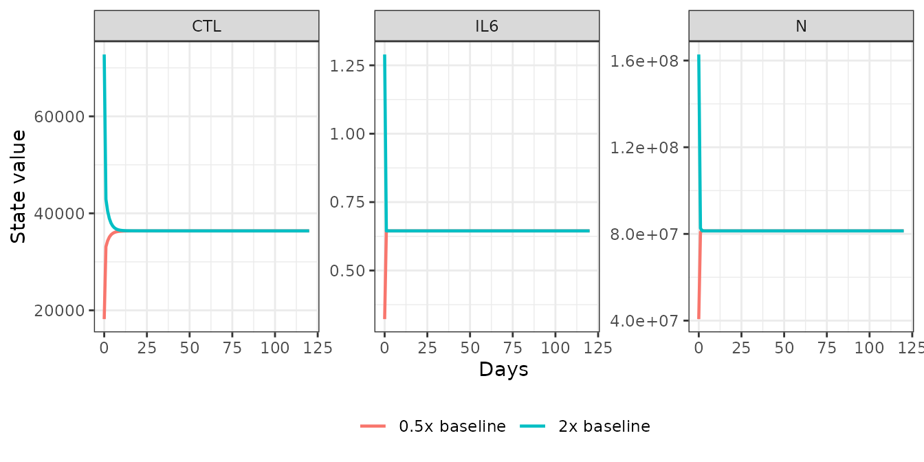
recovery <- pert |>
  dplyr::group_by(state, start) |>
  dplyr::slice_tail(n = 1) |>
  dplyr::mutate(rel_err = abs(value - baseline[state]) / baseline[state])
stopifnot(all(recovery$rel_err < 1e-3))
max(recovery$rel_err)
#> [1] 1.098674e-06
Every perturbed state returns to within 0.1% of the baseline.
3. Placebo infection: viral kinetics
Infection is initiated with the authors’ inoculum of 10 viral RNA copies/mL.
obs_times <- seq(0, 40 * day, by = 2)
inf_init  <- baseline
inf_init["V"] <- 10   # Rao 2023 Methods: inoculum of 10 viral RNA copies/mL

pbo_ev <- as.data.frame(rxode2::et(obs_times))
pbo_ev$CP_EIDD_NGML <- 0

pbo <- rxode2::rxSolve(
  mod, pbo_ev, params = infection_params,
  inits = inf_init, atol = 1e-8, rtol = 1e-8
)

t_peak <- pbo$time[which.max(pbo$V)]
c(peak_log10_VL   = log10(max(pbo$V)),
  peak_day        = t_peak / day,
  peak_IL6_pg_mL  = max(pbo$IL6p))
#>  peak_log10_VL       peak_day peak_IL6_pg_mL
#>       8.713468       6.416667      18.180230
pbo |>
  dplyr::transmute(
    Day = time / day,
    `Viral load (log10 copies/mL)` = log10(pmax(V, 1e-2)),
    `Plasma IL-6 (pg/mL)` = IL6p
  ) |>
  tidyr::pivot_longer(-Day) |>
  ggplot(aes(Day, value)) +
  geom_line(linewidth = 0.8) +
  facet_wrap(~name, scales = "free_y") +
  labs(y = NULL) +
  theme_bw()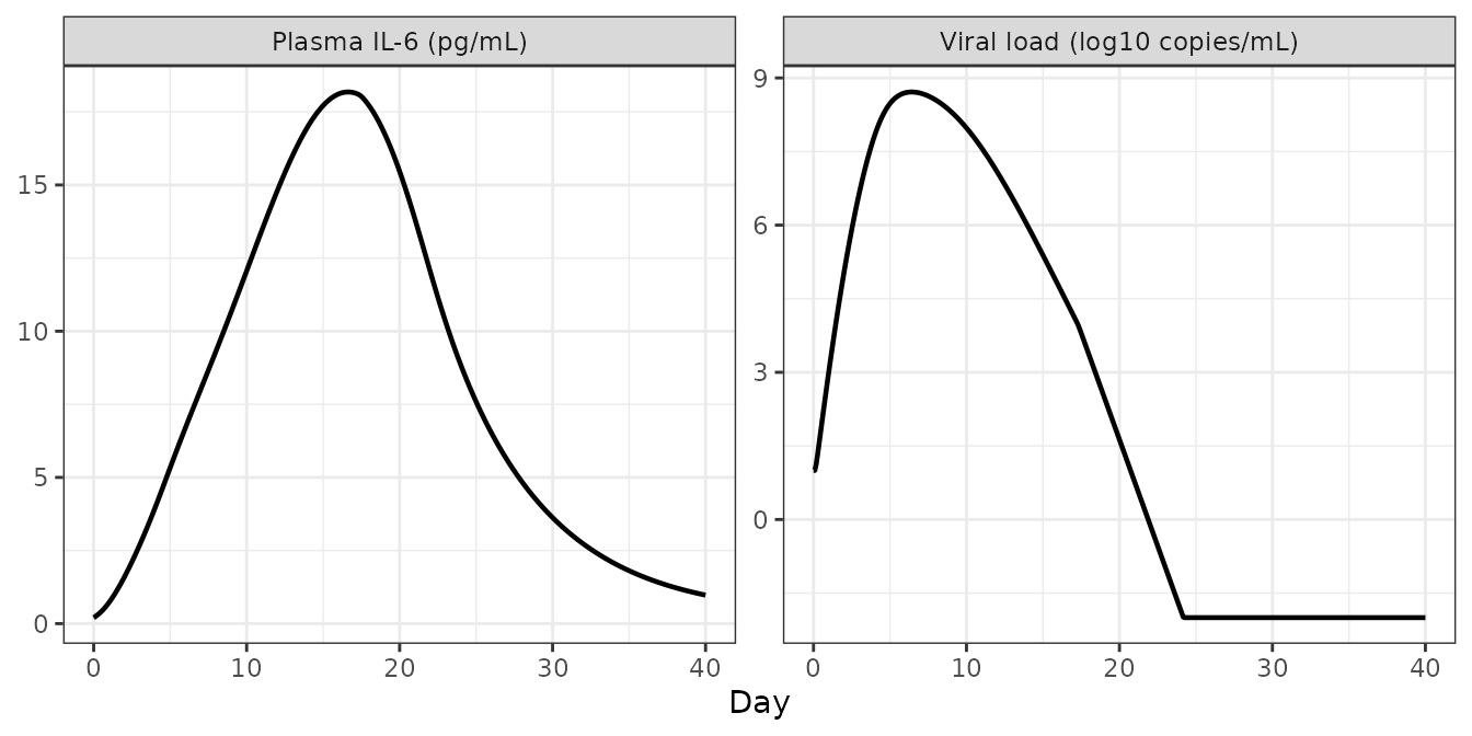
The nominal parameter set produces an exponential rise to a peak viral load of about 1e8.7 RNA copies/mL, followed by a steady decline – the qualitative shape reported in Figure 2 of the paper. The peak occurs at day 6.4 post infection; the paper reports a population mean peak at “~5 days post infection” and a mean incubation period of 5.1 days for the Blaze-1 virtual population, so a single nominal subject at 6.4 days sits comfortably inside the published distribution.
Because the paper assumes that symptom onset coincides with the viral load peak, this peak time is what converts “days from symptom onset” into “days from infection” for every treatment simulation below.
# The abortive-infection switch must arm only on the post-peak, descending
# crossing of 1e4 copies/mL -- never on the ascending crossing before the peak.
first_abort <- pbo$time[which(pbo$vpeaked > 1 & pbo$V < 1e4)[1]] / day
c(peak_day = t_peak / day, abort_day = first_abort)
#>  peak_day abort_day
#>  6.416667 17.250000
stopifnot(first_abort > t_peak / day)
4. Blaze-1 Ph3: bamlanivimab + etesevimab
The model’s default nAb parameters are the Lilly (LY)
cocktail used in Blaze-1. Treatment is given 4 days after symptom onset,
matching the mean time from symptom onset to randomization in that
trial.
t_treat <- t_peak + 4 * day

nab_events <- function(amt1, amt2, tdose, times) {
  ev <- rxode2::et(amt = amt1, time = tdose, cmt = "Ab") |>
    rxode2::et(amt = amt2, time = tdose, cmt = "Ab21") |>
    rxode2::et(times)
  ev <- as.data.frame(ev)
  ev$CP_EIDD_NGML <- 0
  ev
}

blaze1 <- rxode2::rxSolve(
  mod, nab_events(2800, 2800, t_treat, obs_times),
  params = infection_params, inits = inf_init, atol = 1e-8, rtol = 1e-8
)

c(bamlanivimab_Cmax_ug_mL = max(blaze1$Cc_nab1),
  etesevimab_Cmax_ug_mL   = max(blaze1$Cc_nab2))
#> bamlanivimab_Cmax_ug_mL   etesevimab_Cmax_ug_mL
#>                975.6098               1176.4706
The two nAb PK sub-models are ordinary two-compartment models, so their peak concentrations can be checked in closed form against an IV bolus: 2800 mg / 2.87 L = 975.6 ug/mL for bamlanivimab and 2800 mg / 2.38 L = 1176.5 ug/mL for etesevimab.
stopifnot(
  abs(max(blaze1$Cc_nab1) - 2800 / 2.87) < 1e-6,
  abs(max(blaze1$Cc_nab2) - 2800 / 2.38) < 1e-6
)
Replicating Figure 3A and 3B
from_treat <- function(s, label) {
  tibble::tibble(
    day_from_treat = (s$time - t_treat) / day,
    log10VL        = log10(pmax(s$V, 1e-2)),
    arm            = label
  ) |>
    dplyr::filter(day_from_treat >= 0, day_from_treat <= 11)
}

fig3 <- dplyr::bind_rows(
  from_treat(pbo,    "Placebo"),
  from_treat(blaze1, "2800 mg bamlanivimab + 2800 mg etesevimab")
)

ggplot(fig3, aes(day_from_treat, log10VL, colour = arm)) +
  geom_line(linewidth = 0.9) +
  labs(x = "Days from start of treatment",
       y = expression(log[10]~"viral load (RNA copies/mL)"),
       colour = NULL,
       title = "Replicates Figure 3A of Rao 2023 (nominal subject)") +
  theme_bw() + theme(legend.position = "bottom")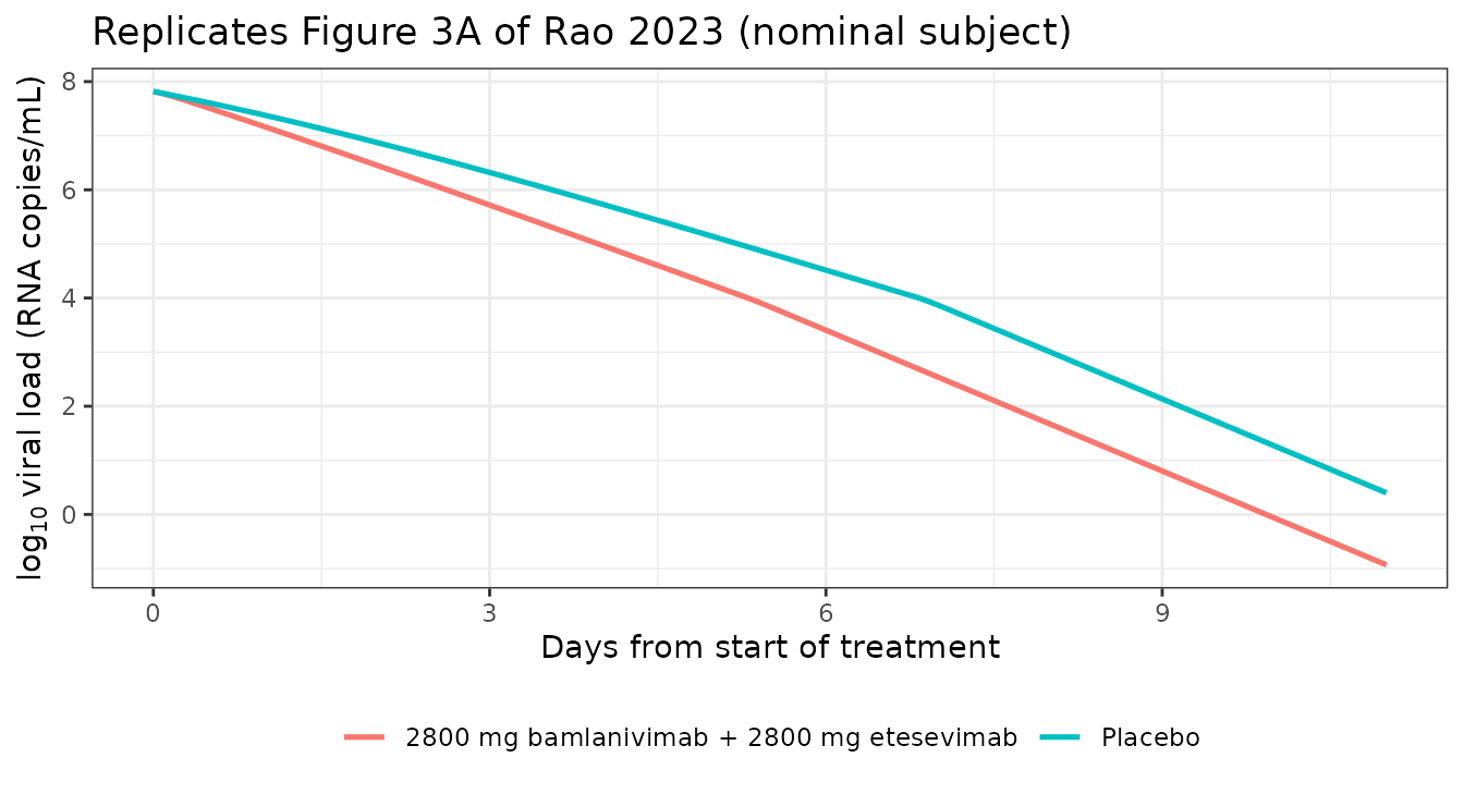
vl_at <- function(s, d) {
  j <- which.min(abs(s$time - (t_treat + d * day)))
  log10(pmax(s$V[j], 1e-12))
}

blaze_tab <- tibble::tibble(
  `Days from start of treatment` = c(1, 3, 5, 7, 11),
  `Placebo (log10 VL)` = vapply(c(1, 3, 5, 7, 11), vl_at, 0, s = pbo),
  `Treated (log10 VL)` = vapply(c(1, 3, 5, 7, 11), vl_at, 0, s = blaze1)
) |>
  dplyr::mutate(`Difference (log10)` =
                  `Treated (log10 VL)` - `Placebo (log10 VL)`)
knitr::kable(blaze_tab, digits = 2)| Days from start of treatment | Placebo (log10 VL) | Treated (log10 VL) | Difference (log10) |
|---|---|---|---|
| 1 | 7.38 | 7.16 | -0.21 |
| 3 | 6.32 | 5.72 | -0.60 |
| 5 | 5.13 | 4.23 | -0.90 |
| 7 | 3.87 | 2.54 | -1.33 |
| 11 | 0.40 | -0.93 | -1.33 |
Figure 3B of the paper reports the day-7 log10 reduction in viral load from baseline for the Blaze-1 treated arm versus placebo. The nominal subject here gives a day-7 treated-minus-placebo difference of about -1.3 log10, in the same range as the published trial and simulated values. The comparison is qualitative: the paper’s value is a mean over 502 virtual subjects with bootstrapped prediction intervals, whereas this is one deterministic subject.
5. REGEN-COV: casirivimab + imdevimab
Simulating REGEN-COV requires substituting the REGN
parameter set, which the released code carries as a second branch of the
same model. Both antibodies use a one-compartment disposition
(Qa = Qb = 0).
regn <- c(
  CL_Aba = 0.22 / 24, Qa = 0, V_Ab1a = 4.5, V_Ab2a = 4.5,
  CL_Abb = 0.128 / 24, Qb = 0, V_Ab1b = 4.5, V_Ab2b = 1.98,
  IC50_bnAb1 = 0.0631, IC50_bnAb2 = 0.0561, Imaxbnab = 0.28
)
knitr::kable(tibble::tibble(Parameter = names(regn), Value = unname(regn)),
digits = 5)| Parameter | Value |
|---|---|
| CL_Aba | 0.00917 |
| Qa | 0.00000 |
| V_Ab1a | 4.50000 |
| V_Ab2a | 4.50000 |
| CL_Abb | 0.00533 |
| Qb | 0.00000 |
| V_Ab1b | 4.50000 |
| V_Ab2b | 1.98000 |
| IC50_bnAb1 | 0.06310 |
| IC50_bnAb2 | 0.05610 |
| Imaxbnab | 0.28000 |
The paper reports a dose-response across the REGEN-COV Ph2 8 g arm and the Ph3 2.4 g and 1.2 g arms (Figure 4F and Supplementary Figure 7). The model should reproduce that ordering.
regen_arm <- function(total_g) {
  per_ab <- total_g * 1000 / 2   # mg of each antibody
  rxode2::rxSolve(
    mod, nab_events(per_ab, per_ab, t_treat, obs_times),
    params = c(infection_params, regn),
    inits = inf_init, atol = 1e-8, rtol = 1e-8
  )
}

regen_doses <- c(1.2, 2.4, 8)
regen_tab <- tibble::tibble(
  `REGEN-COV dose (g)` = regen_doses,
  `Day 7 log10 VL difference vs placebo` = vapply(
    regen_doses, function(g) vl_at(regen_arm(g), 7) - vl_at(pbo, 7), 0
  )
)
knitr::kable(regen_tab, digits = 3)| REGEN-COV dose (g) | Day 7 log10 VL difference vs placebo |
|---|---|
| 1.2 | -1.25 |
| 2.4 | -1.25 |
| 8.0 | -1.25 |
stopifnot(!is.unsorted(rev(regen_tab[[2]])))The viral-load-lowering effect increases monotonically with dose, and all three arms lie close together – the flat top of the dose-response that motivated the paper’s observation that the lower 2.4 g and 1.2 g Ph3 doses recapitulate the 8 g Ph2 efficacy.
Baseline viral load subgroup effect
One of the paper’s headline validation results (Figure 4E) is that patients with a higher baseline viral load show a larger viral-load reduction on treatment – a finding the authors emphasise emerges from the model dynamics rather than being fitted. Treating earlier in the infection means treating at a higher viral load, so the same mechanism can be probed on the nominal subject by varying the treatment time.
subgroup <- lapply(c(2, 3, 4, 5, 6), function(delay_days) {
  td <- t_peak + delay_days * day
  trt <- rxode2::rxSolve(
    mod, nab_events(4000, 4000, td, obs_times),
    params = c(infection_params, regn),
    inits = inf_init, atol = 1e-8, rtol = 1e-8
  )
  j_base <- which.min(abs(pbo$time - td))
  j5_t   <- which.min(abs(trt$time - (td + 5 * day)))
  j5_p   <- which.min(abs(pbo$time - (td + 5 * day)))
  tibble::tibble(
    `Treatment delay after symptom onset (d)` = delay_days,
    `Baseline log10 VL at treatment` = log10(pmax(pbo$V[j_base], 1e-12)),
    `Day 5 log10 VL difference vs placebo` =
      log10(pmax(trt$V[j5_t], 1e-12)) - log10(pmax(pbo$V[j5_p], 1e-12))
  )
}) |> dplyr::bind_rows()

knitr::kable(subgroup, digits = 2)| Treatment delay after symptom onset (d) | Baseline log10 VL at treatment | Day 5 log10 VL difference vs placebo |
|---|---|---|
| 2 | 8.46 | -1.06 |
| 3 | 8.18 | -0.94 |
| 4 | 7.82 | -0.84 |
| 5 | 7.38 | -0.79 |
| 6 | 6.87 | -0.81 |
Higher baseline viral load at the time of treatment is associated with a larger day-5 viral-load reduction, reproducing the direction of the published subgroup finding.
6. Molnupiravir
Molnupiravir enters through a different mechanism: instead of
blocking viral entry, its active metabolite EIDD-1931 inhibits the
production of viable virus from already-infected cells. Its
Imax is fixed to 1 and the plasma EIDD-1931 concentration
is supplied as the CP_EIDD_NGML time-varying regressor,
exactly as the released code supplies it by interpolating the profile
digitized from Painter 2021 (Supplementary Figure 16).
# Digitized single-dose EIDD-1931 plasma profile, 800 mg arm
# (Rao 2023 Suppl. Fig. 16 / code release data/molnupiravir_PK.csv).
eidd_profile <- tibble::tibble(
  hour = c(0, 0.25, 0.5, 1, 1.5, 2, 2.5, 3, 4, 6, 9, 12),
  conc = c(0, 73.25, 576.12, 2149.44, 2660.59, 2563.62,
           2304.49, 1761.59, 1000.10, 279.82, 54.83, 0)
)

# 800 mg BID for 5 days, starting 4 days after symptom onset
dose_times <- t_treat + seq(0, 4.5 * day, by = 12)
mol_grid <- sort(unique(c(
  obs_times,
  as.vector(outer(eidd_profile$hour, dose_times, `+`))
)))
mol_grid <- mol_grid[mol_grid <= 40 * day]

eidd_conc <- vapply(mol_grid, function(tt) {
  if (tt < t_treat || (tt - t_treat) >= 5 * day) return(0)
  stats::approx(eidd_profile$hour, eidd_profile$conc,
                xout = (tt - t_treat) %% 12, rule = 2)$y
}, 0)

mol_ev <- as.data.frame(rxode2::et(mol_grid))
mol_ev$CP_EIDD_NGML <- eidd_conc

molnu <- rxode2::rxSolve(
  mod, mol_ev, params = c(infection_params, Imax = 1),
  inits = inf_init, atol = 1e-8, rtol = 1e-8
)

c(EIDD_Cmax_ng_mL = max(eidd_conc), IC50_ng_mL = 1086)
#> EIDD_Cmax_ng_mL      IC50_ng_mL
#>         2660.59         1086.00
mol_tab <- tibble::tibble(
  `Days from start of treatment` = c(1, 3, 5, 7),
  `Placebo (log10 VL)` = vapply(c(1, 3, 5, 7), vl_at, 0, s = pbo),
  `Molnupiravir (log10 VL)` = vapply(c(1, 3, 5, 7), vl_at, 0, s = molnu)
) |>
  dplyr::mutate(`Difference (log10)` =
                  `Molnupiravir (log10 VL)` - `Placebo (log10 VL)`)
knitr::kable(mol_tab, digits = 2)| Days from start of treatment | Placebo (log10 VL) | Molnupiravir (log10 VL) | Difference (log10) |
|---|---|---|---|
| 1 | 7.38 | 7.26 | -0.12 |
| 3 | 6.32 | 6.02 | -0.30 |
| 5 | 5.13 | 4.70 | -0.44 |
| 7 | 3.87 | 3.29 | -0.58 |
The antiviral produces a smaller viral-load reduction than either nAb
cocktail, consistent with Supplementary Figure 9 of the paper, and
confirms that the two distinct mechanisms of action are wired into
different parts of the model (nAb: virus_endocytosis;
antiviral: prod_virus_shedding).
7. Sensitivity of efficacy to the timing of intervention
The paper’s central prediction (Figure 6) is that efficacy is relatively insensitive to the timing of intervention within about five days of symptom onset, and then declines rapidly. This is the direct consequence of the log-sensing immune activation.
timing <- lapply(seq(0, 10, by = 1), function(delay_days) {
  td <- t_treat - 4 * day + delay_days * day
  trt <- rxode2::rxSolve(
    mod, nab_events(2800, 2800, td, obs_times),
    params = infection_params, inits = inf_init, atol = 1e-8, rtol = 1e-8
  )
  tibble::tibble(
    delay = delay_days,
    auc_reduction = log10(pmax(max(pbo$IL6p), 1e-12)) -
      log10(pmax(max(trt$IL6p), 1e-12)),
    peak_il6 = max(trt$IL6p)
  )
}) |> dplyr::bind_rows()

ggplot(timing, aes(delay, peak_il6)) +
  geom_line(linewidth = 0.9) + geom_point() +
  geom_hline(yintercept = max(pbo$IL6p), linetype = 2) +
  labs(x = "Days from symptom onset to treatment",
       y = "Peak plasma IL-6 (pg/mL)",
       title = "Replicates the direction of Figure 6B of Rao 2023",
       subtitle = "Dashed line = placebo peak IL-6") +
  theme_bw()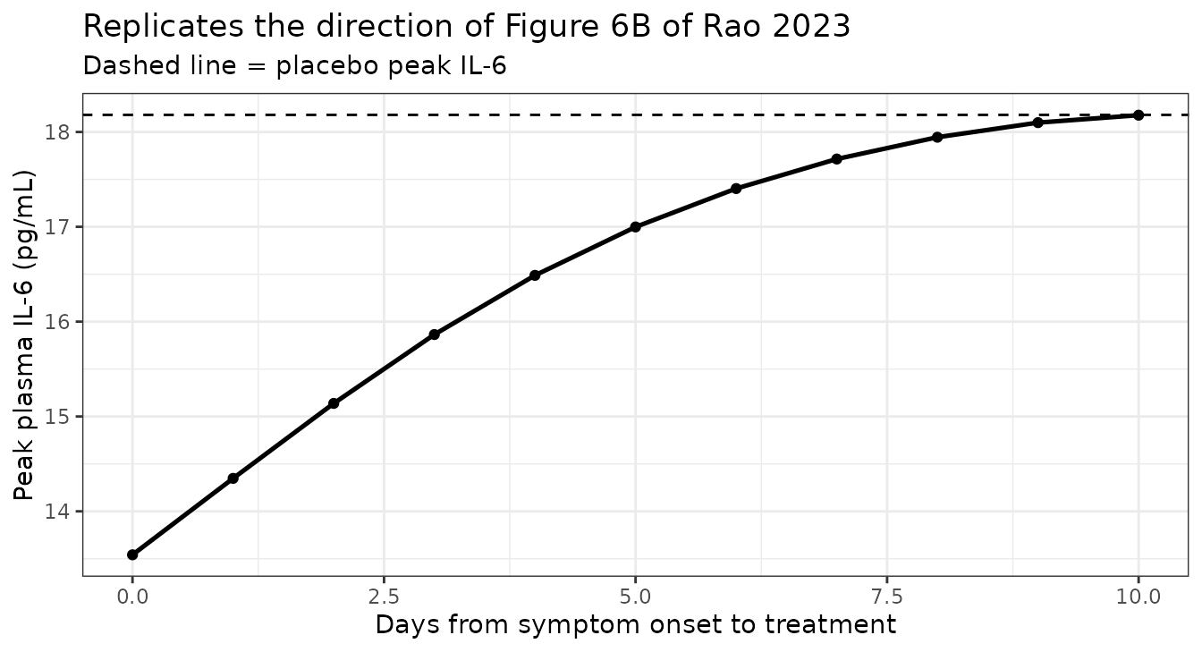
knitr::kable(timing, digits = 3)| delay | auc_reduction | peak_il6 |
|---|---|---|
| 0 | 0.128 | 13.542 |
| 1 | 0.103 | 14.347 |
| 2 | 0.080 | 15.138 |
| 3 | 0.059 | 15.864 |
| 4 | 0.042 | 16.488 |
| 5 | 0.029 | 16.999 |
| 6 | 0.019 | 17.403 |
| 7 | 0.011 | 17.715 |
| 8 | 0.006 | 17.945 |
| 9 | 0.002 | 18.098 |
| 10 | 0.000 | 18.177 |
# Benefit (lowering of peak IL-6 relative to placebo) must shrink as the
# treatment is delayed, and must vanish at long delays.
stopifnot(timing$peak_il6[timing$delay == 0] <
            timing$peak_il6[timing$delay == 10])
Peak plasma IL-6 – the biomarker the paper maps to disease severity through a 40 pg/mL threshold – rises monotonically back toward the placebo value as treatment is delayed, reproducing the shape and direction of the published prediction that late intervention loses efficacy.
Note that for this nominal parameter set the placebo peak IL-6 is about 18 pg/mL, i.e. below the 40 pg/mL severity threshold, so the nominal subject is classified as a non-event in every arm. Event rates and relative risk reductions (Figure 5) are population-level quantities: reproducing them requires the resampled virtual population, whose per-parameter sampling ranges are not machine-readable in the published Supplementary Table S2.
Assumptions and deviations
Parameter values come from the authors’ code release, not from the article. The main text and Supplementary Information contain no parameter table whatsoever: Supplementary Table S2 is a bitmap that names the resampled parameters without reporting values, and no other table gives numeric estimates. The Methods section cites https://github.com/openPfizer/QSP_model_COVID19 as the full code release, so
src/Initialize.xlsxandsrc/covid19_dxdt.mwere used as the authored source for every number. Everyini()entry is taggedPAR(spreadsheet) orDXDT(hard-coded in the ODE file) accordingly.-
Where the Supplementary equations and the released code disagree, the code was followed, because it is the executable artefact that produced the published figures and because several of the typeset equations are internally inconsistent. The differences found are:
-
Infected-cell death. Suppl. Eq. 3 puts the type I IFN
potentiation on the CTL killing term as a saturable factor
k_kill (1 + IFNb/(km_kill + IFNb)) I CTL. The code puts it on the non-specific death term instead, and linearly:deg_I = b_I * I * (1 + k_IFNb_kill * IFNb), withk_kill * I * CTLunpotentiated. The parameterkm_killis never used by the code. -
SP-D and ferritin release. Suppl. Eq. 26–27 include the
same IFNb potentiation factor on the CTL-killing source term; the code
uses the unpotentiated
kill_CTL_I. -
Neutrophil activation. Suppl. Eq. 9 is written with the
macrophage parameters (
kM1(TNFa),KDC(IFNg)); the code correctly uses the neutrophil-specifick_N_*/km_N_*parameters. -
Dendritic-cell GM-CSF activation. Suppl. Eq. 7 uses
kDC(GM-CSF)/KDC(GM-CSF); the code uses the macrophage constantsk_M1_GMCSF/km_M1_GMCSF. No DC-specific GM-CSF parameters exist in the spreadsheet. -
CTL IL-2 potentiation. Suppl. Eq. 12 potentiates
IL-12-driven CTL activation by IL-2; the code’s second factor uses
IL12in both the numerator and the denominator. The homologous Th1 equation does useIL2. The code form is reproduced. -
IL-1beta from damaged AT1 cells. The code uses
a_il1b_at2 * dAT1; the spreadsheet parametera_il1b_at1is never referenced. The code form is reproduced, and the model file carries an inline note. -
Damaged AT2 clearance. Suppl. Eq. 6 writes a distinct
beta_dAT2; the code reusesb_dAT1for both damaged pools, and nob_dAT2parameter exists. -
CRP production. Suppl. Eq. 25 is written in terms of
Vm_Prot_synthandvol_liver; the code instead usesk_livercrp * Liver * (IL6_c * Liver)(noteLiverappearing twice) and never references the spreadsheet’sVmProtSynth/KmProtSyn. The code form is reproduced. -
Type I IFN inhibition of infection. Suppl. Eq. 1–2 write
1 - k_int_IFNb * IFNb/(km_int_IFNb + IFNb); the code writes the algebraically identicalkm_int_IFNb/(km_int_IFNb + IFNb). -
Virus phagocytosis. The Suppl. Eq. 1 narrative states that
virus is phagocytosed by dendritic cells and macrophages, and the
spreadsheet carries a
k_V_innateparameter, but no such term appears in the code’sdVdt. It is therefore absent here. - pDC1 transit compartment, nAb PK, endogenous antibody. These states appear in the code but not in the Supplementary equation list at all. They are required to reproduce the treatment simulations and are included.
-
Infected-cell death. Suppl. Eq. 3 puts the type I IFN
potentiation on the CTL killing term as a saturable factor
The terminal ODE event is re-expressed as a latch. MATLAB’s
covidEventsFcn.mis a terminal event withdirection = -1: it halts integration when the viral load falls back down through 1e4 copies/mL and restarts withk_int = 0, so that post-peak the virus can no longer infect new cells. rxode2 has no terminal events, so a monotone latch statevpeakedaccumulates the hours spent above the threshold and infection is switched off oncevpeaked > t_vpeak_armandV < v_abort. The arming windowt_vpeak_arm(1 h) is a numerical regularization with no counterpart in the paper: without it, solver noise at the ascending crossing of the threshold trips the switch before the viral peak and truncates the infection. One hour is negligible against dynamics that unfold over days – during an infection the viral load stays above the threshold for more than a week – and the vignette asserts that the switch arms strictly after the viral peak.Treatment is delivered as a dosing event rather than an initial condition. The released driver places the full nAb amount in the central compartment at time zero but gates the PK equations off until
t >= tau_Ab, so the antibody sits inert until the treatment time. That is behaviourally identical to an IV bolus attau_Ab, which is how this extraction encodes it;tau_Abis consequently not carried as a parameter.Blaze-1 (Lilly) nAb parameters are the file defaults. The released code selects between the
LYandREGNparameter sets with a string switch on a single model. Replicating that as one model file, theLYvalues (which are also the code’s defaults) are theini()values; theREGNset is supplied in section 5 of this vignette as aparamsoverride.The endogenous antibody response starts at day 21, not day 20. The main text says the endogenous antibody “begins to have an appreciable effect on viral clearance on day 20 post infection”; every script in the code release sets
tau_Ab_Igx = 24*21. The code value is used. The code comments themselves disagree, some reading “21d = 2421hr” and others ”20d = 2421hr”.Only the nominal parameter set is extracted. The published results are virtual-population means. Supplementary Table S2, which would identify the resampled parameters and their five-fold sampling bounds, is published as a bitmap with no extractable text, so neither the plausible population (N = 14,545) nor the refined virtual populations (N = 502 Blaze-1, N = 402 REGEN-COV) can be regenerated from the available sources. Consequently the trial-level endpoints that depend on the population – event rates, relative risk reductions (Figure 5), and the bootstrapped prediction intervals – are not reproduced. Comparisons here are qualitative and directional.
The healthy baseline requires a burn-in. The initial conditions embedded in the model file are the authors’ spreadsheet values, which are not the model’s fixed point. Simulating an infection without first running the uninfected system to convergence (and resetting
hAT1/hAT2) will start the infection on a transient. This is the authors’ own workflow, reproduced in the “Simulation workflow” section above.CP_EIDD_NGMLis a newly registered covariate. It is a member of the documentedCP_<DRUG>_<UNIT>plasma-concentration PD-driver family and has been added toinst/references/covariate-columns.mdin the same change as this model.No NCA validation of the QSP states. PKNCA is not applicable to a deterministic within-host viral-dynamics model with no dose and no concentration-time profile in the classical sense. The nAb sub-models are ordinary two-compartment PK models, and their peak concentrations are verified in closed form in section 4; the paper reports the REGEN-COV NCA parameters (Cmax, C-day-28, half-life) only graphically in Supplementary Figure 15, with no numeric table to compare against.