T-cell engager target-mediated disposition (Penney 2025)
Source:vignettes/articles/Penney_2025_tce_tmdd.Rmd
Penney_2025_tce_tmdd.RmdModel and source
- Citation: Penney M, Ippolito A, Fevola E, Rata S, Brown L, Morentin Gutierrez P, Jones RDO. Predicting the Pharmacokinetics of T-Cell Engagers as a Function of Target-Mediated Drug Disposition. Clin Transl Sci. 2025;18(11):e70384. doi:10.1111/cts.70384. Structural siblings in this library: modellib(‘Betts_2019_pf_06671008_qsp’) and modellib(‘Poels_2025_elranatamab_qsp’).
- Description: QSP. Mechanistic target-mediated drug disposition (TMDD) model predicting the pharmacokinetics of T-cell engagers (TCEs) as a function of target engagement. A two-compartment linear disposition backbone carries mass-action binding of free drug to two independent targets - the CD3 activating receptor on circulating T cells and a tumor-associated antigen (TAA) - each with its own synthesis, internalisation and drug-complex internalisation. Total elimination is the sum of an intrinsic (non-target) clearance plus the two target-mediated routes, which is what makes TCE half-lives much shorter than their IgG-like format would suggest and breaks the usual monkey-to-human allometric ranking. Trimer (CD3 + TAA simultaneous) formation is deliberately omitted by the authors. Defaults are the paper’s generic HUMAN parameterisation in the CD3-binding-only configuration (bl_taa = 0), which is the configuration the authors themselves use for TCEs with no published TAA turnover data (DLL3, GPRC5D) and for Figure 2; set bl_taa / kint_taa / kd_taa to switch the TAA arm on, and thalf_intrinsic to 9 days for the cynomolgus monkey.
- Article: https://doi.org/10.1111/cts.70384
- Supplement: Data S1 (
CTS-18-e70384-s001.docx), Tables S1 / S2, published with the open-access article (PMC12597969).
T-cell engagers (TCEs) are built on IgG-like or albumin-binding formats that should give them half-lives of weeks, yet most clinical-stage TCEs show half-lives of a few days, and the usual “human half-life exceeds monkey half-life” ranking does not hold. Penney et al. explain both observations with target-mediated drug disposition: total elimination is the sum of an intrinsic (non-target) clearance plus target-mediated clearance through the CD3 arm and through the tumor-associated antigen (TAA) arm. Because CD3 and TAA cross-reactivity differ between cynomolgus monkey and human, the dominant elimination route can differ between species, which destroys the allometric correlation.
This vignette reproduces the paper’s generic mechanism results (Figure 2, the only fully-specified quantitative simulation in the paper) and documents two places where the source is internally inconsistent or silent.
Population
This is a prediction method, not a model fitted to a
subject-level dataset, so there is no subject count, no demographic
table, and no inter-individual variability. The generic disposition
parameters are stated assumptions (Sections 2.3, 2.6 and 2.7):
V_C = 40 mL/kg, V_P = 60 mL/kg, Q
= 10 x CL, and CL set from an assumed intrinsic terminal half-life of 15
days in human patients or 9 days in the cynomolgus monkey. The CD3
system parameters are generic literature values (Section 2.3).
The method was evaluated against 29 published clinical-stage TCEs (Table 1) spanning haematological and solid-tumour indications. Prediction accuracy (Table 2) was 18/22 within two-fold for the cynomolgus monkey and 16/18 within two-fold for human patients, versus 10/17 for allometric scaling alone.
The same information is available programmatically via
readModelDb("Penney_2025_tce_tmdd_qsp")()$population.
Source trace
Every ini() entry in
inst/modeldb/pharmacokinetics/Penney_2025_tce_tmdd_qsp.R
carries an in-file comment naming its origin. They are collected here
for review.
| Equation / parameter | Value | Source location |
|---|---|---|
d/dt(central) (free drug D_Free) |
n/a | Equation 1, Section 2.2 |
d/dt(target_cd3_central) (free CD3) |
n/a | Equation 2, Section 2.2 |
d/dt(drug_cd3_central) (drug-CD3 dimer) |
n/a | Equation 3, Section 2.2 |
d/dt(target) (free TAA) |
n/a | Equation 4, Section 2.2 |
d/dt(complex) (drug-TAA dimer) |
n/a | Equation 5, Section 2.2 |
d/dt(peripheral1) (peripheral drug
D_P) |
n/a | Equation 6, Section 2.2 |
CL = ln(2) * (V_C + V_P) / half-life |
derived | Section 2.2 |
k_off = k_on * K_D (both arms) |
derived | Section 2.3 |
lvc |
0.040 L/kg (40 mL/kg) | Sections 2.3, 2.6, 2.7 |
lvp |
0.060 L/kg (60 mL/kg) | Sections 2.3, 2.6, 2.7 |
thalf_intrinsic |
15 day (human); 9 day (cyno) | Sections 2.7 and 2.6 |
qclratio |
10 | Sections 2.3, 2.6, 2.7 |
kon |
86.4 /nM/day (= 1e6 /M/s) | Section 2.3 |
cd3_receptors |
50000 receptors/T cell | Section 2.3 |
tcell_blood |
1500 cells/uL | Section 2.3 |
kint_cd3 |
27.726 /day (= ln 2 / 36 min) | Section 2.3, resolved against the Section 3.2 output (see Errata) |
kd_cd3 |
10 nM | Section 3.2 (representative “first generation” affinity) |
bl_taa |
0 (TAA arm disabled) | Section 2.4 (per-antigen values not reported) |
kint_taa, kd_taa
|
placeholders, inert while bl_taa = 0
|
per-TCE K_D,TAA in Tables S1 / S2 |
Simulation scenarios
The model is deterministic - no eta terms and no
residual error - so there is no virtual cohort and no need for
zeroRe(). Each “subject” below is one scenario
from Figure 2.
mod <- readModelDb("Penney_2025_tce_tmdd_qsp")

# The paper doses in mg/kg but never states a molecular weight for its generic
# TCE, so mg/kg cannot be converted exactly. Doses are therefore given in
# nmol/kg; the mg/kg equivalents shown assume a 150 kDa IgG-like TCE. The
# "MW insensitivity" section below shows this choice does not affect the
# reproduced half-lives at the 0.01 mg/kg dose of Figure 2a.
mw_ref <- 150000                       # g/mol, assumed for LABELLING only
mgkg_to_nmolkg <- function(mgkg, mw = mw_ref) mgkg * 1e-3 / mw * 1e9

obs_grid <- seq(0, 60, by = 0.05)      # days

# Solve one scenario. `cmt = "central"` is the ODE state (never the observable
# name `Cc`); rxode2 returns Cc as a column at those rows automatically.
solve_scenario <- function(label, dose_nmol_kg, ...) {
  ev <- rxode2::et(amt = dose_nmol_kg, cmt = "central")
  ev <- rxode2::et(ev, obs_grid, cmt = "central")
  out <- rxode2::rxSolve(mod, ev, c(...),
                         atol = 1e-12, rtol = 1e-10, maxsteps = 1e6)
  out <- as.data.frame(out)
  # rxSolve omits `id` for a single subject.
  out$id <- 1L
  out$treatment <- label
  out
}

# Terminal half-life by log-linear regression over the last quarter of the
# profile -- well clear of the distribution and TMDD transients. The paper
# computes ln(2) / (-dD_Free/dt / D_Free); on the terminal phase the two agree.
terminal_half_life <- function(df) {
  # Keep Cc >= 1e-6 * Cmax before taking the last quarter: below that the ODE integrator has no relative accuracy left.
  d <- df[df$time > 0 & df$Cc >= 1e-6 * max(df$Cc), ]
  d <- d[d$time >= 0.75 * max(d$time), ]
  as.numeric(log(2) / -coef(stats::lm(log(Cc) ~ time, data = d))[2])
}
Replicate published figures
Figure 2a - half-life falls as CD3 affinity tightens
Figure 2a simulates a single 0.01 mg/kg IV bolus for CD3 affinities
from 1000 nM down to 1 nM in half-log steps, with the TAA arm off. The
paper quotes two of the resulting half-lives in Section 3.2: 15
days at K_D = 1000 nM (i.e. the intrinsic
half-life, because binding is too weak to matter) and 4.4
days at K_D = 10 nM.
kd_grid <- c(1000, 316, 100, 31.6, 10, 3.16, 1)
dose_2a <- mgkg_to_nmolkg(0.01)

sim_2a <- dplyr::bind_rows(lapply(kd_grid, function(kd) {
  solve_scenario(sprintf("%g nM", kd), dose_2a, kd_cd3 = kd)
}))

th_2a <- vapply(split(sim_2a, sim_2a$treatment), terminal_half_life, numeric(1))
th_2a <- th_2a[sprintf("%g nM", kd_grid)]

sim_2a |>
  mutate(treatment = factor(treatment, levels = sprintf("%g nM", kd_grid))) |>
  filter(time > 0) |>
  ggplot(aes(time, Cc, colour = treatment)) +
  geom_line() +
  scale_y_log10() +
  labs(x = "Time (days)", y = "Free TCE concentration (nM)",
       colour = expression(K[D]~"(CD3)"),
       title = "Figure 2a - CD3 affinity drives the observed half-life",
       caption = "Replicates Figure 2a of Penney 2025 (0.01 mg/kg IV bolus, TAA arm off).")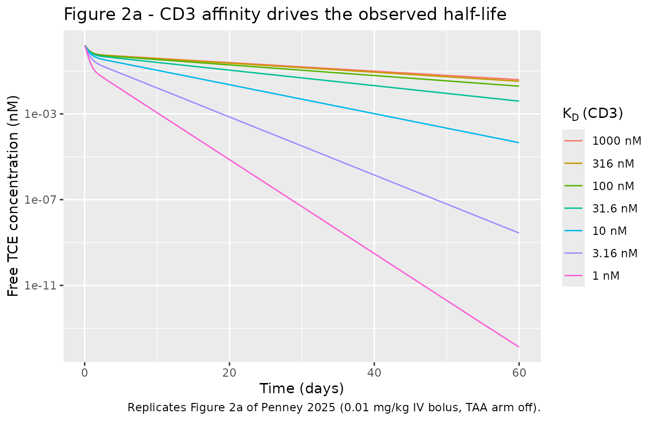
tibble::tibble(
  `K_D CD3 (nM)` = kd_grid,
  `Terminal half-life (day)` = round(as.numeric(th_2a), 2)
) |>
knitr::kable(caption = "Terminal half-life by CD3 affinity (compare Figure 2a legend).")| K_D CD3 (nM) | Terminal half-life (day) |
|---|---|
| 1000.00 | 15.12 |
| 316.00 | 14.26 |
| 100.00 | 12.12 |
| 31.60 | 8.32 |
| 10.00 | 4.45 |
| 3.16 | 2.22 |
| 1.00 | 1.37 |
The two half-lives the paper states in prose are reproduced:
th_1000 <- as.numeric(th_2a["1000 nM"])
th_10 <- as.numeric(th_2a["10 nM"])
stopifnot(
  # Paper: "For a low CD3 binding affinity of 1000 nM ... the TCE displays the
  # half-life of its intrinsic PK of 15 days." Deterministic model, so this is
  # a tight bound (achieved 15.12).
  abs(th_1000 - 15) < 0.5,
  # Paper: "With an affinity of 10 nM ... the half-life is reduced to 4.4 days."
  # Achieved 4.45.
  abs(th_10 - 4.4) < 0.3,
  # Monotone: tighter CD3 binding always shortens the half-life. Deterministic,
  # so step-by-step monotonicity is a legitimate assertion here.
  all(diff(as.numeric(th_2a)) < 0)
)
Figure 2b - raising the dose saturates CD3 and restores the intrinsic half-life
dose_mgkg <- c(0.01, 0.1, 1, 10)

sim_2b <- dplyr::bind_rows(lapply(dose_mgkg, function(d) {
  solve_scenario(sprintf("%g mg/kg", d), mgkg_to_nmolkg(d), kd_cd3 = 10)
}))

th_2b <- vapply(split(sim_2b, sim_2b$treatment), terminal_half_life, numeric(1))
th_2b <- th_2b[sprintf("%g mg/kg", dose_mgkg)]

sim_2b |>
  mutate(treatment = factor(treatment, levels = sprintf("%g mg/kg", dose_mgkg))) |>
  filter(time > 0) |>
  ggplot(aes(time, Cc, colour = treatment)) +
  geom_line() +
  scale_y_log10() +
  labs(x = "Time (days)", y = "Free TCE concentration (nM)", colour = "Dose",
       title = expression("Figure 2b - dose escalation at "*K[D]*"(CD3) = 10 nM"),
       caption = "Replicates Figure 2b of Penney 2025 (TAA arm off).")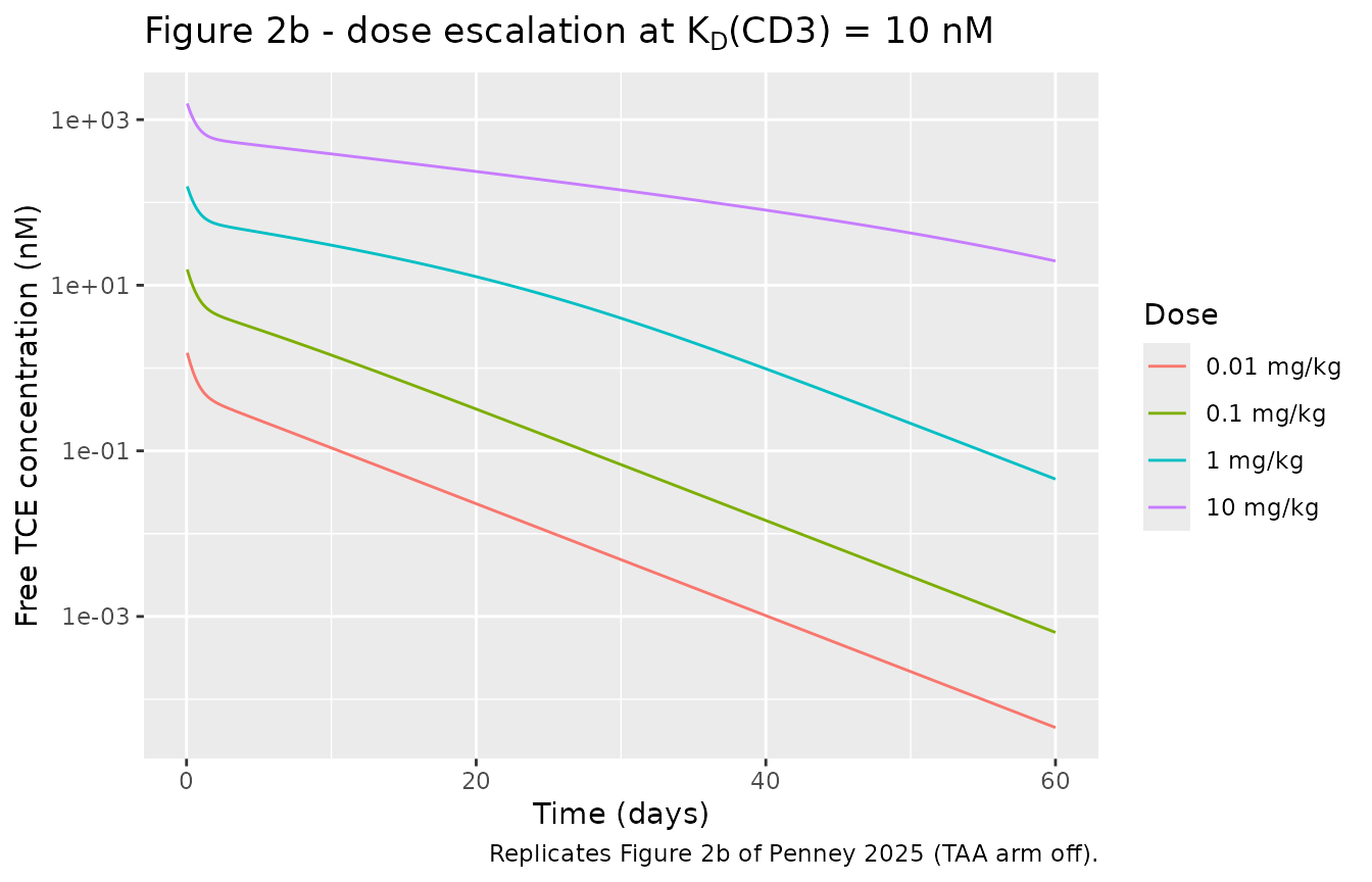
tibble::tibble(
  `Dose (mg/kg, 150 kDa)` = dose_mgkg,
  `Dose (nmol/kg)` = signif(mgkg_to_nmolkg(dose_mgkg), 3),
  `Terminal half-life (day)` = round(as.numeric(th_2b), 2)
) |>
knitr::kable(caption = "Terminal half-life by dose (compare Figure 2b legend).")| Dose (mg/kg, 150 kDa) | Dose (nmol/kg) | Terminal half-life (day) |
|---|---|---|
| 0.01 | 0.0667 | 4.45 |
| 0.10 | 0.6670 | 4.45 |
| 1.00 | 6.6700 | 4.49 |
| 10.00 | 66.7000 | 9.41 |
stopifnot(
  # "at doses below 0.1 mg/kg the PK is essentially linear" -- the 0.01 and
  # 0.1 mg/kg half-lives are indistinguishable.
  abs(as.numeric(th_2b["0.01 mg/kg"]) - as.numeric(th_2b["0.1 mg/kg"])) < 0.05,
  # "even 1 mg/kg showing a reduced half-life with these parameters" -- still
  # far below the 15-day intrinsic value.
  as.numeric(th_2b["1 mg/kg"]) < 7,
  # "Increasing the dose leads to the expected saturation of CD3 and a return
  # to the intrinsic half-life" -- by 10 mg/kg it has moved most of the way back.
  as.numeric(th_2b["10 mg/kg"]) > 7
)
Errata and source-resolution
The CD3 internalisation rate is printed two inconsistent ways
Section 2.3 states that “CD3 internalization rate has been measured by [35] at 1.4%/minute, equating to a half-life of about 36 min”. These two figures cannot both hold: a first-order rate of 0.014/min is a 49.5-minute exponential half-life, not 36 minutes (36 minutes is what 1.4%/min gives if depletion is read as linear, 50 / 1.4 = 35.7 min).
The paper’s own reported model output adjudicates. Only the 36-minute
half-life reading reproduces the quoted 4.4-day half-life at
K_D(CD3) = 10 nM; the 1.4%/min reading gives 5.4 days.
kint_36min <- log(2) / 36 * 1440      # 27.726 /day  -- the packaged default
kint_14pct <- 0.014 * 1440            # 20.160 /day

kint_cmp <- dplyr::bind_rows(lapply(
  list(c(lab = "ln(2)/36 min = 27.726 /day", k = kint_36min),
       c(lab = "1.4 %/min = 20.160 /day", k = kint_14pct)),
  function(x) {
    th <- terminal_half_life(
      solve_scenario(x[["lab"]], dose_2a, kd_cd3 = 10,
                     kint_cd3 = as.numeric(x[["k"]])))
    tibble::tibble(`Reading of the printed rate` = x[["lab"]],
                   `Predicted half-life (day)` = round(th, 2),
                   `Paper states (Section 3.2)` = 4.4)
  }))

knitr::kable(kint_cmp, caption = "Only the 36-minute reading reproduces the paper's own output.")| Reading of the printed rate | Predicted half-life (day) | Paper states (Section 3.2) |
|---|---|---|
| ln(2)/36 min = 27.726 /day | 4.45 | 4.4 |
| 1.4 %/min = 20.160 /day | 5.40 | 4.4 |
stopifnot(
  abs(kint_cmp$`Predicted half-life (day)`[1] - 4.4) < 0.3,   # 36-min reading
  kint_cmp$`Predicted half-life (day)`[2] > 5.0               # 1.4%/min reading
)
The packaged model therefore uses
kint_cd3 = 27.726 /day. This is a resolution of an internal
inconsistency in the source, not a tuned parameter: the value is the
paper’s own stated 36-minute half-life, and it was selected by the
paper’s own stated output, not by fitting anything.
No molecular weight is reported, and it does not matter here
The paper doses in mg/kg throughout but never states a molecular weight for its generic TCE, so mg/kg cannot be converted to molar exactly. At the 0.01 mg/kg dose of Figure 2a the system is in its dose-independent regime (the “fourth phase” of TMDD PK the paper cites), so the predicted half-life is identical across the whole plausible TCE size range - 50 kDa (an albumin-binding construct such as HPN328) to 150 kDa (an IgG-like construct).
mw_check <- vapply(c(50000, 150000), function(mw) {
  terminal_half_life(solve_scenario("mw", mgkg_to_nmolkg(0.01, mw), kd_cd3 = 10))
}, numeric(1))

tibble::tibble(
  `Assumed MW (kDa)` = c(50, 150),
  `0.01 mg/kg as nmol/kg` = signif(mgkg_to_nmolkg(0.01, c(50000, 150000)), 3),
  `Terminal half-life (day)` = round(mw_check, 3)
) |>
knitr::kable(caption = "The Figure 2a anchor is insensitive to the unreported molecular weight.")| Assumed MW (kDa) | 0.01 mg/kg as nmol/kg | Terminal half-life (day) |
|---|---|---|
| 50 | 0.2000 | 4.453 |
| 150 | 0.0667 | 4.453 |
The Figure 2b dose escalation is MW-dependent, because it deliberately leaves the linear regime; its mg/kg labels above assume 150 kDa and should be read as illustrative.
The TAA arm ships disabled because its parameters are not reported
The Table S2 caption states plainly that “actual calibration of the
TAA expression and turnover will not be shown for each TAA but a
reference to the data used will be declared”. The per-antigen TAA burden
(bl_taa) and turnover (kint_taa) are therefore
not recoverable from any published source, and no
non-zero default can be sourced. bl_taa ships at 0, which
disables the arm entirely - this is the authors’ own configuration
whenever TAA data are absent (Section 2.4: for DLL3 and GPRC5D “these
predictions are made for CD3-binding only”) and for Figure 2. Per-TCE
K_D,TAA values are published, in Tables S1 and
S2.
The arm is structurally complete and switches on when the user supplies the two missing values. The illustration below uses round numbers, not paper values.
taa_off <- terminal_half_life(solve_scenario("TAA off", dose_2a, kd_cd3 = 10))
taa_on  <- terminal_half_life(
  solve_scenario("TAA on", dose_2a, kd_cd3 = 10,
                 bl_taa = 0.5, kint_taa = 5, kd_taa = 1))

tibble::tibble(
  Configuration = c("CD3 only (packaged default)",
                    "CD3 + illustrative TAA arm (bl_taa = 0.5 nM, kint_taa = 5 /day)"),
  `Terminal half-life (day)` = round(c(taa_off, taa_on), 2)
) |>
knitr::kable(caption = "Adding a second target-mediated route shortens the half-life further.")| Configuration | Terminal half-life (day) |
|---|---|
| CD3 only (packaged default) | 4.45 |
| CD3 + illustrative TAA arm (bl_taa = 0.5 nM, kint_taa = 5 /day) | 1.40 |
# Mechanism check: a second elimination route can only shorten the half-life.
stopifnot(taa_on < taa_off)
PKNCA validation
PKNCA recomputes the terminal half-life independently of the log-linear fit used above, and supplies Cmax and AUC for the Figure 2a scenarios.
sim_nca <- sim_2a |>
  dplyr::filter(!is.na(Cc)) |>
  dplyr::select(id, time, Cc, treatment) |>
  # Per scenario, keep Cc >= 1e-6 * Cmax after the peak (and time zero): below that the ODE integrator has no relative accuracy left.
  dplyr::group_by(treatment, id) |>
  dplyr::filter(time == 0 | time <= time[which.max(Cc)] | Cc >= 1e-6 * max(Cc)) |>
  dplyr::ungroup()

# Guarantee a time = 0 row per (id, treatment). For an IV bolus into a
# concentration state the t = 0 record is already present, but the bind/distinct
# idiom is kept so the filter can never silently drop the AUC anchor.
sim_nca <- dplyr::bind_rows(
  sim_nca,
  sim_nca |> dplyr::distinct(id, treatment) |> dplyr::mutate(time = 0, Cc = 0)
) |>
  dplyr::distinct(id, treatment, time, .keep_all = TRUE) |>
  dplyr::arrange(treatment, id, time)

conc_obj <- PKNCA::PKNCAconc(sim_nca, Cc ~ time | treatment + id)

dose_df <- sim_2a |>
  dplyr::distinct(id, treatment) |>
  dplyr::mutate(time = 0, amt = dose_2a)

dose_obj <- PKNCA::PKNCAdose(dose_df, amt ~ time | treatment + id)

intervals <- data.frame(
  start = 0, end = Inf,
  cmax = TRUE, tmax = TRUE, aucinf.obs = TRUE, half.life = TRUE
)

nca_res <- PKNCA::pk.nca(PKNCA::PKNCAdata(conc_obj, dose_obj, intervals = intervals))
Comparison against the published half-lives
Penney et al. report only two numeric half-lives for the generic simulation (Section 3.2); the remaining Figure 2a values appear solely in the figure legend, which is a raster image, so they are not transcribed here.
published <- tibble::tribble(
  ~treatment,  ~half.life,
  "1000 nM",   15.0,
  "10 nM",      4.4
)

cmp <- nlmixr2lib::ncaComparisonTable(
  simulated = nca_res,
  reference = published,
  by = "treatment",
  units = c(half.life = "day", cmax = "nM", tmax = "day", aucinf.obs = "nM*day"),
  tolerance_pct = 20
)

knitr::kable(
  cmp,
  caption = "Simulated vs. published terminal half-life. * differs from reference by >20%."
)| NCA parameter | treatment | Reference | Simulated | % diff |
|---|---|---|---|---|
| t½ (day) | 1000 nM | 15 | 15.1 | +0.6% |
| t½ (day) | 10 nM | 4.4 | 4.45 | +1.1% |
No row is starred: both published half-lives are reproduced well inside 20%.
hl <- as.data.frame(nca_res)
hl <- hl[hl$PPTESTCD == "half.life", ]
hl_1000 <- hl$PPORRES[hl$treatment == "1000 nM"]
hl_10 <- hl$PPORRES[hl$treatment == "10 nM"]

# Guard against a lookup that silently matched nothing.
stopifnot(length(hl_1000) == 1L, length(hl_10) == 1L)

# PKNCA's terminal-slope selection must agree with the regression above.
stopifnot(
  abs(hl_1000 - th_1000) < 0.5,
  abs(hl_10 - th_10) < 0.5
)
Assumptions and deviations
-
kint_cd3resolves an internal inconsistency in the source. Section 2.3 prints “1.4%/minute” and “a half-life of about 36 min”, which disagree. The packaged value 27.726 /day isln(2) / 36 min, selected because it is the only reading that reproduces the paper’s own quoted 4.4-day output atK_D(CD3) = 10 nM (the 1.4%/min reading gives 5.4 days). See the Errata section for the demonstration. No parameter was tuned. -
The TAA arm ships disabled
(
bl_taa = 0). The authors state in the Table S2 caption that the calibrated per-antigen TAA expression and turnover are not reported, so no value can be sourced.kint_taaandkd_taaare inert placeholders whilebl_taa = 0, labelled as such. Per-TCEK_D,TAAvalues are available in Tables S1 and S2 for users switching the arm on. - No molecular weight is reported, so doses are in nmol/kg rather than mg/kg. The Figure 2a anchors are shown above to be insensitive to this over the 50-150 kDa range; the Figure 2b mg/kg labels assume 150 kDa and are illustrative only.
- Trimer formation is omitted, following the authors (Section 2.2): they implemented the Jiang trimer model and found “a negligble difference to the predicted half-life”, so it was dropped. The packaged model reproduces that choice rather than reinstating it.
-
The model is body-weight normalised (volumes in
L/kg, doses in nmol/kg) because the paper is. There is no
WTcovariate; scaling is implicit. -
The whole model is deterministic. The source
reports no residual-error model and no inter-individual variability, so
propSdisfixed(0)and there are noetaterms. The supplement does describe a virtual-population sensitivity analysis (lognormal draws on intrinsic half-life, CD3 and TAA expression and bothK_Dvalues, calibrated so 95% of values fall within three-fold of the mean); that is a sensitivity exercise rather than an estimated variance model, and it depends on the unreported GUCY2C TAA parameters, so it is not reproduced here. -
The cynomolgus-monkey configuration is the same
model with
thalf_intrinsic = 9days (Section 2.6) instead of 15. -
Per-TCE application is not reproduced. Reproducing
an individual TCE from Table S1 / S2 needs that molecule’s dose and
molecular weight, which the tables do not carry; only
K_Dvalues and observed / predicted half-lives are tabulated. -
target_cd3_centralis a new canonical compartment registered with this extraction (inst/references/compartment-names.md). Penney 2025 carries free CD3 as a dynamic turnover state, whereas its siblingsBetts_2019_pf_06671008_qspandPoels_2025_elranatamab_qspderive free CD3 algebraically from a T-cell density. It is named into the existing free-target family besidetarget_bonemarrowrather than as a barecd3_central, so that the free receptor pool stays distinct from the drug-bounddrug_cd3_centraldimer it binds to (maintainer decision, 2026-09-11).