Relative efficacy of biologic DMARDs in rheumatoid arthritis (Mandema 2011)
Source:vignettes/articles/Mandema_2011_biologicDMARDs_mbma.Rmd
Mandema_2011_biologicDMARDs_mbma.RmdModel and source
- Citation: Mandema JW, Salinger DH, Baumgartner SW, Gibbs MA. A dose-response meta-analysis for quantifying relative efficacy of biologics in rheumatoid arthritis. Clin Pharmacol Ther. 2011;90(6):828-835. doi:10.1038/clpt.2011.256. The model equations are in the Methods section ‘Analysis methodology’ (p. 834). The Supplementary Data is a list of the 50 included trials and contains no parameter estimates.
- Article: https://doi.org/10.1038/clpt.2011.256
- Supplement: a list of the 50 included trials with PubMed IDs. It contains no parameter estimates.
This is a model-based meta-analysis (MBMA), not a population PK model. It has no PK layer, no ODE states, no between-subject variability and no residual error model. The unit of prediction is a study arm, and the outputs are per-arm ACR responder probabilities.
Population
Mandema and colleagues pooled 50 randomized controlled trials in adults with rheumatoid arthritis (RA), covering 21,529 patients, nine biologic disease-modifying antirheumatic drugs (DMARDs) across five mechanisms of action, and methotrexate (MTX) as a tenth randomized treatment. All 50 trials reported ACR 20 responder rates; 49 reported ACR 50 and 45 reported ACR 70. Each trial contributed its response at its own pre-determined primary time point (34 trials at 22-30 weeks, 13 at 12-16 weeks, 4 at one year), which is why the model has no time axis.
Thirty-six trials enrolled patients with an inadequate response to MTX, nine enrolled MTX-naive patients, and five enrolled patients with an inadequate response to MTX and/or a prior anti-TNF. Forty trials were placebo-controlled. Only one of the 50 trials compared two biologics head to head (infliximab vs. abatacept), which is the whole motivation for the indirect comparison.
The same information is available programmatically from the model’s
population metadata
(readModelDb("Mandema_2011_biologicDMARDs_mbma")()$population
- readModelDb() returns the model function, so the
trailing () evaluates it).
pop <- readModelDb("Mandema_2011_biologicDMARDs_mbma")()$population
tibble::tibble(
  Field = c("Patients", "Trials", "Randomized treatments",
            "Trials reporting ACR 20 / 50 / 70", "Placebo-controlled trials"),
  Value = c(format(pop$n_subjects, big.mark = ","), pop$n_studies,
            pop$n_treatments,
            paste(pop$n_trials_acr20, pop$n_trials_acr50, pop$n_trials_acr70,
                  sep = " / "),
            pop$n_trials_placebo_ctl)
) |>
knitr::kable(caption = "Analysis data set (Mandema 2011 Table 1 and Results).")| Field | Value |
|---|---|
| Patients | 21,529 |
| Trials | 50 |
| Randomized treatments | 10 |
| Trials reporting ACR 20 / 50 / 70 | 50 / 49 / 45 |
| Placebo-controlled trials | 40 |
Model structure
Per-arm responder counts were assumed binomial, and the probability
that a patient in arm j of trial i attains ACR
endpoint k was modelled on the logit scale as a trial
placebo response plus a treatment effect (Mandema 2011 Methods,
p. 834):
with f the inverse logit. The placebo response is an ACR
50 fixed effect per trial plus logit-scale shifts for the other two
endpoints,
,
where
has mean
.
The treatment effect is an Emax function of the arm’s normalized
dose:
The single structural finding that organizes the whole paper is in that equation: Emax is a property of the mechanism of action and ED50 is a property of the drug. All five anti-TNFs share one dose-response shape and differ only in where their approved dose sits on it.
Three further terms complete the model:
- the three ACR endpoints share one ED50 and differ only by a multiplicative scaling of the treatment effect (the source tested “differences in Emax and/or ED50 between ACR 20, 50, and 70” and retained a difference in Emax only);
- initial combination therapy of a biologic with MTX is sub-additive, with ;
- covariates act on Emax as ; the only covariate retained was an East Asian trial-location indicator worth a 33% larger treatment effect.
Recovering the unpublished parameters
Mandema 2011 publishes its equations but no parameter
table, and its supplement is a trial list. Every value in
ini() was therefore recovered by inverting the paper’s own
printed results. This section reproduces that recovery; it is the part
of this vignette that most deserves a reviewer’s attention.
Step 1: the treatment effect at each drug’s starting dose
Table 2 gives the absolute difference from placebo in ACR 20/50/70 at each biologic’s suggested starting dose, for a typical placebo response of 24%, 8.6% and 2.7%. Because the model is a logit-scale shift, the treatment effect follows in closed form: .
logit  <- function(p) log(p / (1 - p))
ilogit <- function(x) 1 / (1 + exp(-x))

p0 <- c(acr20 = 0.240, acr50 = 0.086, acr70 = 0.027)   # Mandema 2011 p. 830

table2 <- tibble::tribble(
  ~drug,          ~dose, ~acr20, ~acr50, ~acr70,
  "anakinra",       100,   15.5,    9.5,    4.0,
  "golimumab",       50,   21.3,   13.9,    6.2,
  "tocilizumab",      4,   25.7,   17.7,    8.2,
  "abatacept",       10,   27.1,   18.9,    8.9,
  "infliximab",       3,   28.5,   20.3,    9.7,
  "adalimumab",      40,   29.2,   20.9,   10.0,
  "rituximab",     1000,   33.2,   25.0,   12.6,
  "etanercept",      25,   37.1,   29.3,   15.5,
  "certolizumab",   200,   40.4,   33.3,   18.4
)

geff <- table2 |>
  dplyr::mutate(
    g20 = logit(p0[["acr20"]] + acr20 / 100) - logit(p0[["acr20"]]),
    g50 = logit(p0[["acr50"]] + acr50 / 100) - logit(p0[["acr50"]]),
    g70 = logit(p0[["acr70"]] + acr70 / 100) - logit(p0[["acr70"]])
  )
Step 2: the endpoint scaling acts on Emax, not on ED50
If the endpoint difference acted on ED50, the ratio would vary with dose/ED50 - and the nine drugs span roughly 0.3 to 17 times their own ED50. If it acts on Emax, the ratio is a constant. It is a constant, to within the 0.1-percentage-point rounding of Table 2:
scales <- geff |>
  dplyr::transmute(drug, s20 = g20 / g50, s70 = g70 / g50)

s20 <- sum(geff$g20 * geff$g50) / sum(geff$g50^2)   # least squares through 0
s70 <- sum(geff$g70 * geff$g50) / sum(geff$g50^2)

# Constant across nine drugs spanning a 50-fold range of dose/ED50: this is the
# evidence that the endpoint difference is an Emax difference, exactly as the
# source states ("no statistically significant differences in ... ED50 between
# ACR 20, 50, and 70").
stopifnot(
  max(abs(scales$s20 - s20)) < 0.01,
  max(abs(scales$s70 - s70)) < 0.01
)

scales |>
  dplyr::mutate(dplyr::across(c(s20, s70), \(x) round(x, 4))) |>
  dplyr::rename("Drug" = drug, "ACR 20 / ACR 50" = s20, "ACR 70 / ACR 50" = s70) |>
  knitr::kable(caption = paste0(
    "Endpoint scaling of the treatment effect, per drug. Least-squares values ",
    "used in the model: ", round(s20, 4), " and ", round(s70, 4), "."
))| Drug | ACR 20 / ACR 50 | ACR 70 / ACR 50 |
|---|---|---|
| anakinra | 0.8506 | 1.1135 |
| golimumab | 0.8557 | 1.1171 |
| tocilizumab | 0.8557 | 1.1129 |
| abatacept | 0.8584 | 1.1145 |
| infliximab | 0.8562 | 1.1136 |
| adalimumab | 0.8583 | 1.1103 |
| rituximab | 0.8576 | 1.1135 |
| etanercept | 0.8580 | 1.1134 |
| certolizumab | 0.8570 | 1.1125 |
Step 3: the anti-TNF Emax, four independent ways
The Discussion prints how far up its own curve each anti-TNF is dosed: “golimumab is dosed at 1.1 (0.6 to 1.9; 95% CI) times, infliximab at 2.1 (1.3 to 3.4) times, adalimumab at 2.2 (1.4 to 3.5) times, etanercept at 6.8 (3.4 to 15) times, and certolizumab at >10 times the ED50.” For a drug at times its ED50, , so each ratio implies the shared class Emax on its own. Four independent implications, one shared parameter:
ratio_pub <- c(golimumab = 1.1, infliximab = 2.1, adalimumab = 2.2,
               etanercept = 6.8)
g50 <- setNames(geff$g50, geff$drug)

emax_implied <- g50[names(ratio_pub)] * (1 + 1 / ratio_pub)
emax_antitnf <- mean(emax_implied)

# Four separate published ratios must agree on one Emax if the paper's central
# claim (all anti-TNFs share a dose-response, differing only in potency) holds.
spread <- (max(emax_implied) - min(emax_implied)) / emax_antitnf
stopifnot(spread < 0.02)

tibble::tibble(
  Drug = names(emax_implied),
  `Published dose/ED50` = unname(ratio_pub),
  `Implied anti-TNF Emax` = round(unname(emax_implied), 4)
) |>
  knitr::kable(caption = paste0(
    "Anti-TNF Emax implied independently by each published dose/ED50 ratio. ",
    "Spread ", round(100 * spread, 1), "%; mean ", round(emax_antitnf, 4),
    " is the value used in the model."
))| Drug | Published dose/ED50 | Implied anti-TNF Emax |
|---|---|---|
| golimumab | 1.1 | 2.1510 |
| infliximab | 2.1 | 2.1600 |
| adalimumab | 2.2 | 2.1706 |
| etanercept | 6.8 | 2.1446 |
That 1.2% spread is what makes the recovery credible: it is a four-fold-overdetermined system that the paper never intended as a consistency check, and it closes.
Step 4: the four single-drug classes, from Figure 2
Anakinra, abatacept, rituximab and tocilizumab are each the only member of their mechanism-of-action class, so Table 2 gives one equation in two unknowns for each. The missing information is the curvature, which is drawn in Figure 2. The published curves were digitized from a 600-dpi render of page 830: the 3x3 panel grid was located from the black axis frames, each panel calibrated from its printed tick marks, and the ACR 20 / 50 / 70 curves fitted jointly for one (Emax, ED50) pair per panel by maximizing the number of curve pixels within 4 pixels of the prediction.
Accuracy control. The five anti-TNF panels were digitized by the identical procedure and their Emax is already known from Step 3, so the digitization error is measured rather than assumed: the digitized anti-TNF Emax averaged 2.205 against the algebraic 2.157, a bias of +2.2%. The ED50 is the weaker of the two: it is only well determined where the curve is bending, so for drugs dosed far above their ED50 the digitized ratio scattered by up to 30% (etanercept, at 8.8 digitized versus 6.8 published).
The model therefore takes only the Emax from the digitization and sets each ED50 to the value that makes the digitized Emax reproduce that drug’s published Table 2 effect exactly. All the digitization uncertainty lands where Figure 2 is actually informative (the curvature), and none of it lands on the published Table 2 anchor.
emax_digitized <- c(anakinra = 0.954, abatacept = 1.747,
                    rituximab = 1.869, tocilizumab = 5.604)

anchor_ed50 <- function(drug, emax) {
  d <- table2$dose[table2$drug == drug]
  g <- g50[[drug]]
  d * (emax - g) / g
}

recovered <- tibble::tibble(
  drug = names(emax_digitized),
  emax = unname(emax_digitized),
  ed50 = vapply(names(emax_digitized),
                \(d) anchor_ed50(d, emax_digitized[[d]]), numeric(1))
) |>
  dplyr::mutate(
    dose      = table2$dose[match(drug, table2$drug)],
    dose_ed50 = dose / ed50
  )

recovered |>
  dplyr::mutate(dplyr::across(c(emax, ed50, dose_ed50), \(x) signif(x, 4))) |>
  dplyr::select("Drug" = drug, "Class Emax" = emax, "ED50" = ed50,
                "Starting dose" = dose, "Dose/ED50" = dose_ed50) |>
  knitr::kable(caption = paste0(
    "Single-drug classes: Emax digitized from Figure 2, ED50 anchored on ",
    "Table 2. ED50 units follow each drug's own regimen (mg/day, mg/kg q4w, ",
    "mg at weeks 0 and 2, mg/kg q4w)."
))| Drug | Class Emax | ED50 | Starting dose | Dose/ED50 |
|---|---|---|---|---|
| anakinra | 0.954 | 11.720 | 100 | 8.5300 |
| abatacept | 1.747 | 2.532 | 10 | 3.9500 |
| rituximab | 1.869 | 111.000 | 1000 | 9.0110 |
| tocilizumab | 5.604 | 12.820 | 4 | 0.3121 |
Tocilizumab is the striking one. Its ED50 lands above the entire studied 2-8 mg/kg range, which is the quantitative content of two separate statements in the paper - that its theoretical Emax is significantly greater than the anti-TNFs’, and that doubling its dose buys far more response than doubling an anti-TNF dose. Both are tested below.
Step 5: the MTX-naive population
Table 3 reports the difference from MTX for five biologic monotherapies in MTX-naive patients, and the Discussion states that MTX monotherapy itself gives 32, 24 and 12 percentage-point absolute differences from placebo in that population. That is six constraints on two unknowns per endpoint (the MTX-naive placebo response, and the MTX effect), so the system is over-determined:
mtx_delta <- c(acr20 = 0.32, acr50 = 0.24, acr70 = 0.12)  # Mandema 2011 p. 833

table3 <- tibble::tribble(
  ~drug,         ~acr20, ~acr50, ~acr70,
  "golimumab",     -9.8,   -9.2,   -5.3,
  "tocilizumab",   -5.4,   -5.3,   -3.2,
  "infliximab",    -2.6,   -2.7,   -1.6,
  "adalimumab",    -2.0,   -2.0,   -1.3,
  "etanercept",     5.8,    6.5,    4.4
)

solve_naive <- function(ep) {
  gd  <- setNames(geff[[paste0("g", substr(ep, 4, 5))]], geff$drug)[table3$drug]
  tgt <- mtx_delta[[ep]] + table3[[ep]] / 100     # biologic minus placebo
  obj <- function(p) sum((ilogit(logit(p) + gd) - (p + tgt))^2)
  p   <- optimize(obj, c(1e-3, 0.6))$minimum
  list(p0 = p,
       g_mtx = logit(p + mtx_delta[[ep]]) - logit(p),
       resid_pp = 100 * (ilogit(logit(p) + gd) - (p + tgt)))
}

naive <- lapply(c("acr20", "acr50", "acr70"), solve_naive)
names(naive) <- c("acr20", "acr50", "acr70")

# Five Table 3 rows over-determine one unknown per endpoint. If the recovered
# treatment effects were wrong, these residuals would not close.
stopifnot(max(abs(unlist(lapply(naive, `[[`, "resid_pp")))) < 0.15)

naive_tab <- tibble::tibble(
  Endpoint = c("ACR 20", "ACR 50", "ACR 70"),
  `Placebo response (%)` = round(100 * vapply(naive, `[[`, numeric(1), "p0"), 2),
  `MTX-IR placebo (%)`   = 100 * p0,
  `MTX effect (logit)`   = round(vapply(naive, `[[`, numeric(1), "g_mtx"), 4),
  `Max |residual| (pp)`  = round(vapply(naive, \(x) max(abs(x$resid_pp)),
                                        numeric(1)), 3)
)
knitr::kable(naive_tab, caption = paste0(
  "MTX-naive population recovered from Table 3 plus the 32/24/12 ",
  "percentage-point MTX statement."
))| Endpoint | Placebo response (%) | MTX-IR placebo (%) | MTX effect (logit) | Max |residual| (pp) |
|---|---|---|---|---|
| ACR 20 | 26.83 | 24.0 | 1.3602 | 0.065 |
| ACR 50 | 9.27 | 8.6 | 1.5853 | 0.104 |
| ACR 70 | 2.91 | 2.7 | 1.7650 | 0.079 |
Two independent confirmations fall out of this. First, the recovered MTX-naive placebo response is larger than the MTX-inadequate-responder placebo response for all three endpoints, which is precisely the explanation the paper gives for Figure 4: “the absolute effect of an anti-TNF was slightly greater in MTX-naive patients because of a slightly larger placebo response in these patients.” Second, the recovered MTX effects scale across endpoints by 0.858 and 1.113, matching the biologic endpoint scalings of 0.857 and 1.113 that were fitted from an entirely different table - as the paper requires (“no statistically significant difference across the mechanisms of action with respect to the difference between ACR 20, 50, and 70 responses”).
Source trace
| Parameter | Value | Source |
|---|---|---|
| e0_acr50 | -2.3635 | Table 2 footnote, 8.6% typical ACR 50 placebo response (p. 830) |
| theta_acr20 | 1.2108 | Table 2 footnote, 24% ACR 20 placebo response |
| theta_acr70 | -1.2211 | Table 2 footnote, 2.7% ACR 70 placebo response |
| e0_acr50_naive | -2.2814 | Derived: Table 3 + ‘32, 24, and 12%’ MTX statement (p. 833) |
| theta_acr20_naive | 1.2781 | Derived: as above |
| theta_acr70_naive | -1.2250 | Derived: as above |
| scale_acr20 | 0.8570 | Derived: least squares over the 27 cells of Table 2 |
| scale_acr70 | 1.1132 | Derived: least squares over the 27 cells of Table 2 |
| emax_antitnf | 2.1566 | Derived: Table 2 + the four Discussion dose/ED50 ratios (p. 833) |
| emax_antiil1 | 0.954 | Digitized: Figure 2 anakinra panel (p. 830) |
| emax_cd28 | 1.747 | Digitized: Figure 2 abatacept panel |
| emax_cd20 | 1.869 | Digitized: Figure 2 rituximab panel |
| emax_antiil6 | 5.604 | Digitized: Figure 2 tocilizumab panel |
| led50_adalimumab | log(17.81) | Derived: emax_antitnf anchored on the Table 2 adalimumab row |
| led50_certolizumab | log(11.78) | Derived: emax_antitnf anchored on the Table 2 certolizumab row |
| led50_etanercept | log(3.836) | Derived: emax_antitnf anchored on the Table 2 etanercept row |
| led50_golimumab | log(45.70) | Derived: emax_antitnf anchored on the Table 2 golimumab row |
| led50_infliximab | log(1.421) | Derived: emax_antitnf anchored on the Table 2 infliximab row |
| led50_anakinra | log(11.72) | Derived: emax_antiil1 anchored on the Table 2 anakinra row |
| led50_abatacept | log(2.532) | Derived: emax_cd28 anchored on the Table 2 abatacept row |
| led50_rituximab | log(111.0) | Derived: emax_cd20 anchored on the Table 2 rituximab row |
| led50_tocilizumab | log(12.82) | Derived: emax_antiil6 anchored on the Table 2 tocilizumab row |
| e_mtx | 1.5853 | Derived: Table 3 + ‘32, 24, and 12%’ MTX statement (p. 833) |
| gamma_mtx | -0.32 | PRINTED: ‘The interaction coefficient gamma … was -0.32 (-0.37 to -0.27)’ (p. 831) |
| beta_eastasia | 0.33 | PRINTED: ‘significantly (33% (95% CI, 12 to 54%)) greater’ (p. 831) |
| Emax model | g = Emax_class * Dose / (Dose + ED50_drug) | Methods, ‘Analysis methodology’ (p. 834) |
| Placebo structure | E0,ki = E0,i + h_i,k, mean theta_k | Methods, ‘Analysis methodology’ (p. 834) |
| Combination model | g = g_bio + g_MTX + gamma * g_bio * g_MTX | Methods, ‘Analysis methodology’ (p. 834) |
| Covariate model | Emax,i = Emax,class * (1 + theta_c * (X - Xbar) + eta) | Methods, ‘Analysis methodology’ (p. 834) |
Virtual cohort
There is no subject-level cohort to simulate: the model predicts study-arm outcomes. The “cohort” is a grid of study arms - one row per (treatment, dose, population, region) combination.
covariate_names <- c(
  "CONMED_ABATACEPT_DOSE", "CONMED_ADALIMUMAB_DOSE", "CONMED_ANAKINRA_DOSE",
  "CONMED_CERTOLIZUMAB_DOSE", "CONMED_ETANERCEPT_DOSE", "CONMED_GOLIMUMAB_DOSE",
  "CONMED_INFLIXIMAB_DOSE", "CONMED_RITUXIMAB_DOSE", "CONMED_TOCILIZUMAB_DOSE",
  "CONMED_MTX_DOSE", "REGION_EASTASIA"
)

# Drug -> (dose column, mechanism of action, studied dose range from Table 1).
drug_table <- tibble::tribble(
  ~drug,          ~column,                    ~moa,        ~lo,  ~hi,
  "abatacept",    "CONMED_ABATACEPT_DOSE",    "anti-CD28",  0.5,   10,
  "adalimumab",   "CONMED_ADALIMUMAB_DOSE",   "anti-TNF",    20,  160,
  "anakinra",     "CONMED_ANAKINRA_DOSE",     "anti-IL-1",    3,  162,
  "certolizumab", "CONMED_CERTOLIZUMAB_DOSE", "anti-TNF",   200,  400,
  "etanercept",   "CONMED_ETANERCEPT_DOSE",   "anti-TNF",   0.5,   50,
  "golimumab",    "CONMED_GOLIMUMAB_DOSE",    "anti-TNF",    50,  200,
  "infliximab",   "CONMED_INFLIXIMAB_DOSE",   "anti-TNF",     2,   20,
  "rituximab",    "CONMED_RITUXIMAB_DOSE",    "anti-CD20",  500, 1000,
  "tocilizumab",  "CONMED_TOCILIZUMAB_DOSE",  "anti-IL-6",    2,    8
)

# One study arm per row: every covariate column is 0 except those named.
make_arms <- function(label, ..., n = 1L) {
  set <- list(...)
  zeros <- as.list(rep(0, length(covariate_names)))
  names(zeros) <- covariate_names
  for (nm in names(set)) zeros[[nm]] <- set[[nm]]
  out <- tibble::as_tibble(zeros)[rep(1, n), ]
  dplyr::bind_cols(tibble::tibble(arm = label, time = 0, evid = 0), out)
}

# 1. Placebo (no randomized treatment at all).
arms_placebo <- make_arms("placebo")

# 2. Each biologic at its Table 2 suggested starting dose.
arms_start <- dplyr::bind_rows(lapply(seq_len(nrow(table2)), function(i) {
  d <- table2$drug[i]
  col <- drug_table$column[drug_table$drug == d]
  a <- make_arms(paste0("start:", d))
  a[[col]] <- table2$dose[i]
  a
}))

# 3. MTX monotherapy, and each biologic monotherapy or biologic + MTX, in the
#    MTX-naive setting (Tables 3 and 4).
arms_mtx <- make_arms("mtx", CONMED_MTX_DOSE = 18)
arms_combo <- dplyr::bind_rows(lapply(c("golimumab", "infliximab",
                                        "adalimumab", "etanercept"),
                                      function(d) {
  col <- drug_table$column[drug_table$drug == d]
  a <- make_arms(paste0("combo:", d), CONMED_MTX_DOSE = 18)
  a[[col]] <- table2$dose[table2$drug == d]
  a
}))

# 4. A dose grid per drug, spanning each drug's studied range, for the figures.
n_grid <- 60L
arms_grid <- dplyr::bind_rows(lapply(seq_len(nrow(drug_table)), function(i) {
  info <- drug_table[i, ]
  grid <- exp(seq(log(info$hi / 200), log(info$hi), length.out = n_grid))
  a <- make_arms(paste0("grid:", info$drug), n = n_grid)
  a[[info$column]] <- grid
  a$grid_dose <- grid
  a$grid_drug <- info$drug
  a$grid_moa <- info$moa
  a
}))

# 5. The East Asian trials: etanercept at its starting dose, with and without.
arms_asia <- dplyr::bind_rows(
  {a <- make_arms("asia:row");      a$CONMED_ETANERCEPT_DOSE <- 25; a},
  {a <- make_arms("asia:eastasia", REGION_EASTASIA = 1)
   a$CONMED_ETANERCEPT_DOSE <- 25; a}
)

arms <- dplyr::bind_rows(arms_placebo, arms_start, arms_mtx, arms_combo,
                         arms_grid, arms_asia) |>
  dplyr::mutate(id = dplyr::row_number(), .before = 1)

cat("study arms simulated:", nrow(arms), "\n")
#> study arms simulated: 557
Simulation
# Compile once: this vignette solves the model many times with different
# single-arm covariate sets, and re-deriving the ui each time is wasted work.
mod <- rxode2::rxode(readModelDb("Mandema_2011_biologicDMARDs_mbma"))

sim <- rxode2::rxSolve(
  mod,
  events = as.data.frame(dplyr::select(arms, -"grid_dose", -"grid_drug",
                                       -"grid_moa")),
  keep = "arm",
  returnType = "data.frame"
) |>
  tibble::as_tibble() |>
  # rxSolve returns `id` as a factor for a multi-subject solve; coerce back so
  # the join against the arm table matches on value rather than on level order.
  dplyr::mutate(id = as.integer(as.character(id))) |>
  dplyr::left_join(dplyr::select(arms, id, grid_dose, grid_drug, grid_moa),
                   by = "id")

# The model is deterministic: no etas, no residual error. One row per arm.
stopifnot(nrow(sim) == nrow(arms))

get_arm <- function(label) sim[sim$arm == label, ]
The placebo arm reproduces both intercepts exactly
A placebo arm sets every dose column to 0, which collapses the treatment effect to zero and leaves the per-endpoint placebo response. This is an exact check of the intercept encoding for both reported populations.
plc <- get_arm("placebo")

placebo_check <- tibble::tibble(
  Endpoint = c("ACR 20", "ACR 50", "ACR 70"),
  `MTX-IR simulated (%)`    = 100 * c(plc$p_acr20, plc$p_acr50, plc$p_acr70),
  `MTX-IR published (%)`    = 100 * unname(p0),
  `MTX-naive simulated (%)` = 100 * c(plc$p_acr20_naive, plc$p_acr50_naive,
                                      plc$p_acr70_naive),
  `MTX-naive recovered (%)` = 100 * vapply(naive, `[[`, numeric(1), "p0")
)

stopifnot(
  max(abs(placebo_check$`MTX-IR simulated (%)` -
          placebo_check$`MTX-IR published (%)`)) < 1e-3,
  max(abs(placebo_check$`MTX-naive simulated (%)` -
          placebo_check$`MTX-naive recovered (%)`)) < 1e-3
)

placebo_check |>
  dplyr::mutate(dplyr::across(where(is.numeric), \(x) round(x, 2))) |>
knitr::kable(caption = "Placebo (control) arm responder rates.")| Endpoint | MTX-IR simulated (%) | MTX-IR published (%) | MTX-naive simulated (%) | MTX-naive recovered (%) |
|---|---|---|---|---|
| ACR 20 | 24.0 | 24.0 | 26.83 | 26.83 |
| ACR 50 | 8.6 | 8.6 | 9.27 | 9.27 |
| ACR 70 | 2.7 | 2.7 | 2.91 | 2.91 |
Replicate Table 2: efficacy at the suggested starting dose
Table 2 is the paper’s headline result: the absolute difference from placebo at each biologic’s suggested starting dose, in patients with an inadequate response to prior MTX.
The ACR 50 column is reproduced by construction - each ED50 was anchored on it - so it carries no information. The ACR 20 and ACR 70 columns do: they are predicted from the single pair of endpoint scale factors fitted across all nine drugs, so an error in the multiplicative-Emax structure would show up there.
t2_sim <- table2 |>
  dplyr::rowwise() |>
  dplyr::mutate(
    row = list(get_arm(paste0("start:", drug))),
    sim20 = 100 * (row$p_acr20 - plc$p_acr20),
    sim50 = 100 * (row$p_acr50 - plc$p_acr50),
    sim70 = 100 * (row$p_acr70 - plc$p_acr70)
  ) |>
  dplyr::ungroup() |>
  dplyr::select(-row)

d20 <- t2_sim$sim20 - t2_sim$acr20
d50 <- t2_sim$sim50 - t2_sim$acr50
d70 <- t2_sim$sim70 - t2_sim$acr70

# ACR 50 is exact by construction; ACR 20 and ACR 70 are genuine predictions
# and must land inside twice the 0.1-percentage-point rounding of Table 2.
stopifnot(
  max(abs(d50)) < 0.05,
  max(abs(d20)) < 0.60,
  max(abs(d70)) < 0.30
)

t2_sim |>
  dplyr::transmute(
    Drug = drug,
    `Dose` = dose,
    `ACR 20 pub` = acr20, `ACR 20 sim` = round(sim20, 1),
    `ACR 50 pub` = acr50, `ACR 50 sim` = round(sim50, 1),
    `ACR 70 pub` = acr70, `ACR 70 sim` = round(sim70, 1)
  ) |>
  knitr::kable(caption = paste0(
    "Mandema 2011 Table 2: absolute difference in ACR response from placebo ",
    "(percentage points). Largest deviation ",
    round(max(abs(c(d20, d50, d70))), 2), " percentage points."
))| Drug | Dose | ACR 20 pub | ACR 20 sim | ACR 50 pub | ACR 50 sim | ACR 70 pub | ACR 70 sim |
|---|---|---|---|---|---|---|---|
| anakinra | 100 | 15.5 | 15.6 | 9.5 | 9.5 | 4.0 | 4.0 |
| golimumab | 50 | 21.3 | 21.3 | 13.9 | 13.9 | 6.2 | 6.2 |
| tocilizumab | 4 | 25.7 | 25.7 | 17.7 | 17.7 | 8.2 | 8.2 |
| abatacept | 10 | 27.1 | 27.1 | 18.9 | 18.9 | 8.9 | 8.9 |
| infliximab | 3 | 28.5 | 28.5 | 20.3 | 20.3 | 9.7 | 9.7 |
| adalimumab | 40 | 29.2 | 29.2 | 20.9 | 20.9 | 10.0 | 10.0 |
| rituximab | 1000 | 33.2 | 33.2 | 25.0 | 25.0 | 12.6 | 12.6 |
| etanercept | 25 | 37.1 | 37.1 | 29.3 | 29.3 | 15.5 | 15.5 |
| certolizumab | 200 | 40.4 | 40.4 | 33.3 | 33.3 | 18.4 | 18.4 |
The anti-TNFs recover their published dose/ED50 ratios
The five anti-TNF ED50 values were derived from a shared Emax that came from the Discussion ratios, not from Table 2 alone, so re-deriving those ratios from the fitted model is a genuine round trip.
tnf <- c("golimumab", "infliximab", "adalimumab", "etanercept", "certolizumab")
ratio_sim <- vapply(tnf, \(d) get_arm(paste0("start:", d))$dose_over_ed50,
                    numeric(1))

ratio_check <- tibble::tibble(
  Drug = tnf,
  Published = c("1.1", "2.1", "2.2", "6.8", ">10"),
  Simulated = round(unname(ratio_sim), 2)
)

# Point estimates: within 6% of the published value. Certolizumab has only a
# lower bound published, which the model must clear.
stopifnot(
  max(abs(ratio_sim[names(ratio_pub)] / ratio_pub - 1)) < 0.06,
  ratio_sim[["certolizumab"]] > 10
)

knitr::kable(ratio_check, caption = paste0(
  "Dose/ED50 at the suggested starting dose, model versus Mandema 2011 ",
  "Discussion (p. 833)."
))| Drug | Published | Simulated |
|---|---|---|
| golimumab | 1.1 | 1.09 |
| infliximab | 2.1 | 2.11 |
| adalimumab | 2.2 | 2.25 |
| etanercept | 6.8 | 6.52 |
| certolizumab | >10 | 16.98 |
Replicate Table 3: biologic monotherapy versus MTX in MTX-naive patients
mtx_row <- get_arm("mtx")

# MTX monotherapy versus placebo must reproduce the printed 32 / 24 / 12
# percentage-point differences.
mtx_vs_plc <- 100 * c(
  mtx_row$p_acr20_naive - plc$p_acr20_naive,
  mtx_row$p_acr50_naive - plc$p_acr50_naive,
  mtx_row$p_acr70_naive - plc$p_acr70_naive
)
stopifnot(max(abs(mtx_vs_plc - 100 * mtx_delta)) < 0.15)

t3_sim <- table3 |>
  dplyr::rowwise() |>
  dplyr::mutate(
    row = list(get_arm(paste0("start:", drug))),
    sim20 = 100 * (row$p_acr20_naive - mtx_row$p_acr20_naive),
    sim50 = 100 * (row$p_acr50_naive - mtx_row$p_acr50_naive),
    sim70 = 100 * (row$p_acr70_naive - mtx_row$p_acr70_naive)
  ) |>
  dplyr::ungroup() |>
  dplyr::select(-row)

t3_dev <- with(t3_sim, c(sim20 - acr20, sim50 - acr50, sim70 - acr70))
stopifnot(max(abs(t3_dev)) < 0.30)

t3_sim |>
  dplyr::transmute(
    Drug = drug,
    `ACR 20 pub` = acr20, `ACR 20 sim` = round(sim20, 1),
    `ACR 50 pub` = acr50, `ACR 50 sim` = round(sim50, 1),
    `ACR 70 pub` = acr70, `ACR 70 sim` = round(sim70, 1)
  ) |>
  knitr::kable(caption = paste0(
    "Mandema 2011 Table 3: absolute difference in ACR response from MTX for ",
    "biologic monotherapy in MTX-naive patients (percentage points). Largest ",
    "deviation ", round(max(abs(t3_dev)), 2), " percentage points. MTX ",
    "monotherapy itself is ", paste(round(mtx_vs_plc, 1), collapse = " / "),
    " percentage points above placebo, versus the published 32 / 24 / 12."
))| Drug | ACR 20 pub | ACR 20 sim | ACR 50 pub | ACR 50 sim | ACR 70 pub | ACR 70 sim |
|---|---|---|---|---|---|---|
| golimumab | -9.8 | -9.7 | -9.2 | -9.3 | -5.3 | -5.4 |
| tocilizumab | -5.4 | -5.3 | -5.3 | -5.3 | -3.2 | -3.2 |
| infliximab | -2.6 | -2.6 | -2.7 | -2.7 | -1.6 | -1.6 |
| adalimumab | -2.0 | -1.9 | -2.0 | -2.0 | -1.3 | -1.3 |
| etanercept | 5.8 | 5.8 | 6.5 | 6.6 | 4.4 | 4.5 |
Etanercept is the only biologic monotherapy that beats MTX monotherapy, and golimumab and tocilizumab are significantly worse than it - the model reproduces the sign pattern as well as the magnitudes.
Replicate Table 4: initial combination therapy with MTX
Table 4 is the first genuine out-of-sample test in this vignette. Nothing about the combination arms was used to recover any parameter: the interaction coefficient is printed in the paper, and everything it acts on was fitted from Tables 2 and 3.
table4 <- tibble::tribble(
  ~drug,        ~acr20, ~acr50, ~acr70,
  "golimumab",    12.2,   13.1,    8.4,
  "infliximab",   15.5,   17.4,   11.6,
  "adalimumab",   15.7,   17.7,   11.9,
  "etanercept",   19.1,   22.5,   15.8
)

t4_sim <- table4 |>
  dplyr::rowwise() |>
  dplyr::mutate(
    row = list(get_arm(paste0("combo:", drug))),
    sim20 = 100 * (row$p_acr20_naive - mtx_row$p_acr20_naive),
    sim50 = 100 * (row$p_acr50_naive - mtx_row$p_acr50_naive),
    sim70 = 100 * (row$p_acr70_naive - mtx_row$p_acr70_naive)
  ) |>
  dplyr::ungroup() |>
  dplyr::select(-row)

t4_dev <- with(t4_sim, c(sim20 - acr20, sim50 - acr50, sim70 - acr70))

# Fully out of sample; require agreement within 0.6 percentage points.
stopifnot(max(abs(t4_dev)) < 0.60)

# Table 4 also pins down WHERE the endpoint scaling enters the interaction.
# Forming the product on the ACR 50 scale and scaling the result afterwards
# gives a materially different, and wrong, answer -- so this is a real
# structural discrimination, not a rounding preference.
alt_scaled <- t4_sim |>
  dplyr::rowwise() |>
  dplyr::mutate(
    bio  = list(get_arm(paste0("start:", drug))),
    g50c = bio$lor_acr50 + mtx_row$lor_acr50 -
           0.32 * bio$lor_acr50 * mtx_row$lor_acr50,
    alt20 = 100 * (ilogit(logit(plc$p_acr20_naive) + s20 * g50c) -
                   mtx_row$p_acr20_naive)
  ) |>
  dplyr::ungroup()

stopifnot(max(abs(alt_scaled$alt20 - alt_scaled$acr20)) > 1.0)

# Sub-additivity must hold: the combination is less than the sum of its parts.
combo_subadditive <- vapply(table4$drug, function(d) {
  cb <- get_arm(paste0("combo:", d))
  bi <- get_arm(paste0("start:", d))
  cb$lor_acr50 < bi$lor_acr50 + mtx_row$lor_acr50 - 1e-8
}, logical(1))
stopifnot(all(combo_subadditive))

t4_sim |>
  dplyr::transmute(
    Drug = drug,
    `ACR 20 pub` = acr20, `ACR 20 sim` = round(sim20, 1),
    `ACR 50 pub` = acr50, `ACR 50 sim` = round(sim50, 1),
    `ACR 70 pub` = acr70, `ACR 70 sim` = round(sim70, 1)
  ) |>
  knitr::kable(caption = paste0(
    "Mandema 2011 Table 4: absolute difference in ACR response from MTX for ",
    "initial combination therapy in MTX-naive patients (percentage points). ",
    "Largest deviation ", round(max(abs(t4_dev)), 2),
    " percentage points, entirely out of sample."
))| Drug | ACR 20 pub | ACR 20 sim | ACR 50 pub | ACR 50 sim | ACR 70 pub | ACR 70 sim |
|---|---|---|---|---|---|---|
| golimumab | 12.2 | 12.3 | 13.1 | 13.2 | 8.4 | 8.3 |
| infliximab | 15.5 | 15.6 | 17.4 | 17.4 | 11.6 | 11.3 |
| adalimumab | 15.7 | 15.8 | 17.7 | 17.7 | 11.9 | 11.6 |
| etanercept | 19.1 | 19.1 | 22.5 | 22.3 | 15.8 | 15.3 |
The source writes the interaction on the endpoint-specific functions, , so the product is formed after the endpoint scaling. That is not a distinction one can settle from the equation’s typography alone, but Table 4 settles it empirically: forming the product on the ACR 50 scale and scaling the result afterwards misses the published ACR 20 column by up to 2 percentage points, against 0.47 for the form used here. Monotherapy arms are unaffected either way, because the product term vanishes.
Replicate Figure 2: the dose-response curves
grid_long <- sim |>
  dplyr::filter(!is.na(grid_drug)) |>
  dplyr::select(grid_drug, grid_dose, p_acr20, p_acr50, p_acr70) |>
  tidyr::pivot_longer(dplyr::starts_with("p_acr"),
                      names_to = "endpoint", values_to = "p") |>
  dplyr::mutate(endpoint = factor(endpoint,
                                  levels = c("p_acr20", "p_acr50", "p_acr70"),
                                  labels = c("ACR 20", "ACR 50", "ACR 70")))

start_pts <- table2 |>
  tidyr::pivot_longer(c(acr20, acr50, acr70), names_to = "endpoint",
                      values_to = "delta") |>
  dplyr::mutate(
    endpoint = factor(endpoint, levels = c("acr20", "acr50", "acr70"),
                      labels = c("ACR 20", "ACR 50", "ACR 70")),
    p = delta / 100 + rep(unname(p0), times = nrow(table2))
  ) |>
  dplyr::rename(grid_drug = drug, grid_dose = dose)

ggplot(grid_long, aes(grid_dose, 100 * p, colour = endpoint)) +
  geom_line(linewidth = 0.7) +
  geom_point(data = start_pts, size = 2, shape = 21, fill = "white") +
  facet_wrap(~grid_drug, scales = "free_x", ncol = 3) +
  scale_colour_manual(values = c("ACR 20" = "black", "ACR 50" = "blue",
                                 "ACR 70" = "red")) +
  coord_cartesian(ylim = c(0, 80)) +
  labs(x = "Dose (each drug in its own standard-regimen units)",
       y = "Percent achieving ACR response", colour = NULL,
       title = "Replicates Figure 2 of Mandema 2011",
       subtitle = paste("Lines: model. Points: the Table 2 suggested",
                        "starting dose.")) +
  theme_bw() +
  theme(legend.position = "top")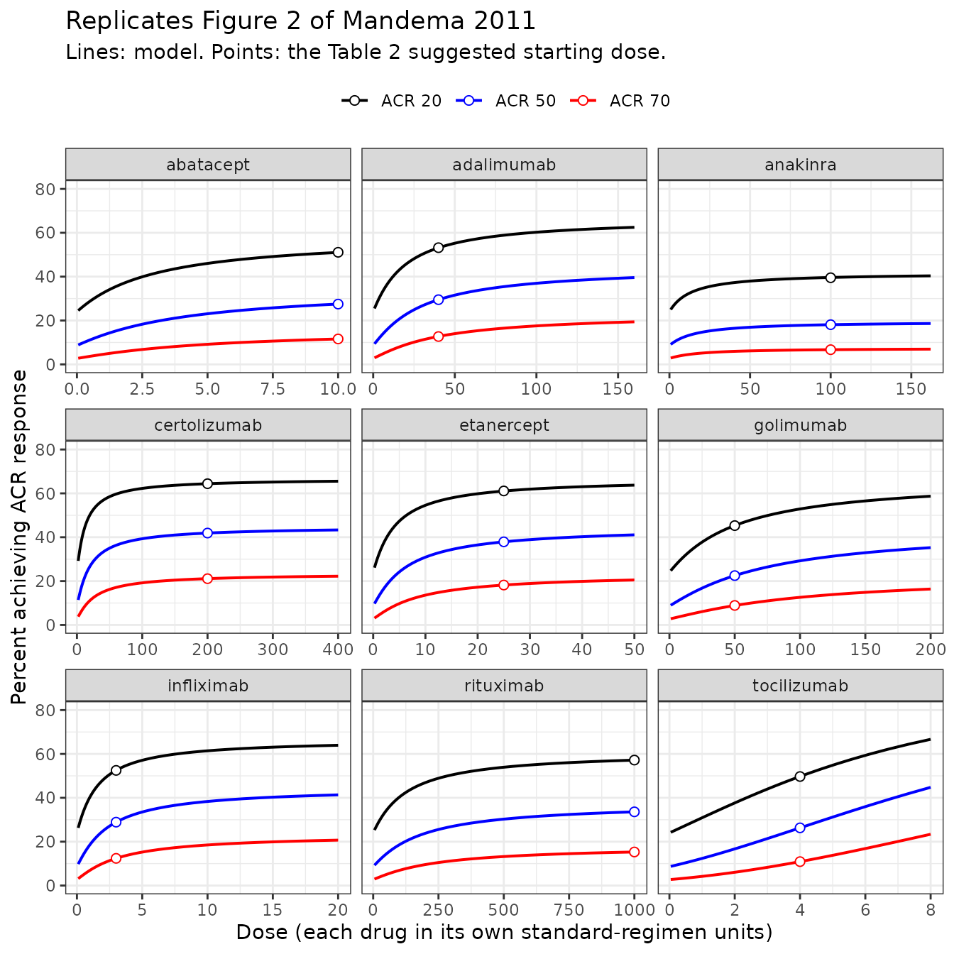
Two features of the published figure must survive: every curve starts from the placebo response at dose 0, and the ordering ACR 20 > ACR 50 > ACR 70 holds at every dose.
stopifnot(
  all(grid_long$p > 0 & grid_long$p < 1),
  with(sim[!is.na(sim$grid_drug), ],
       all(p_acr20 > p_acr50 & p_acr50 > p_acr70)),
  # Monotone increasing in dose for every drug and every endpoint.
  all(vapply(split(grid_long, list(grid_long$grid_drug, grid_long$endpoint)),
             \(d) all(diff(d$p[order(d$grid_dose)]) > 0), logical(1)))
)
Replicate Figure 3: one link between ACR 20 and ACR 50
Figure 3 plots ACR 20 against ACR 50 across every drug and shows that they all fall on a single continuous curve - the paper’s evidence that “there was also no statistically significant difference across the mechanisms of action with respect to the difference between ACR 20, 50, and 70 responses”.
In the fitted model this is an identity rather than an approximation. Because the endpoint scaling acts on Emax and the ED50 is shared, , which involves no drug-specific quantity at all. Every drug must lie on the same curve to machine precision.
link <- sim |>
  dplyr::filter(!is.na(grid_drug)) |>
  dplyr::select(grid_drug, grid_moa, p_acr20, p_acr50)

ggplot(link, aes(100 * p_acr50, 100 * p_acr20, colour = grid_moa,
                 group = grid_drug)) +
  geom_line(linewidth = 0.8, alpha = 0.8) +
  labs(x = "Percent achieving ACR 50", y = "Percent achieving ACR 20",
       colour = NULL, title = "Replicates Figure 3 of Mandema 2011",
       subtitle = paste("All nine biologics trace the same ACR 20 / ACR 50",
                        "link, irrespective of mechanism of action.")) +
  theme_bw() +
  theme(legend.position = "top")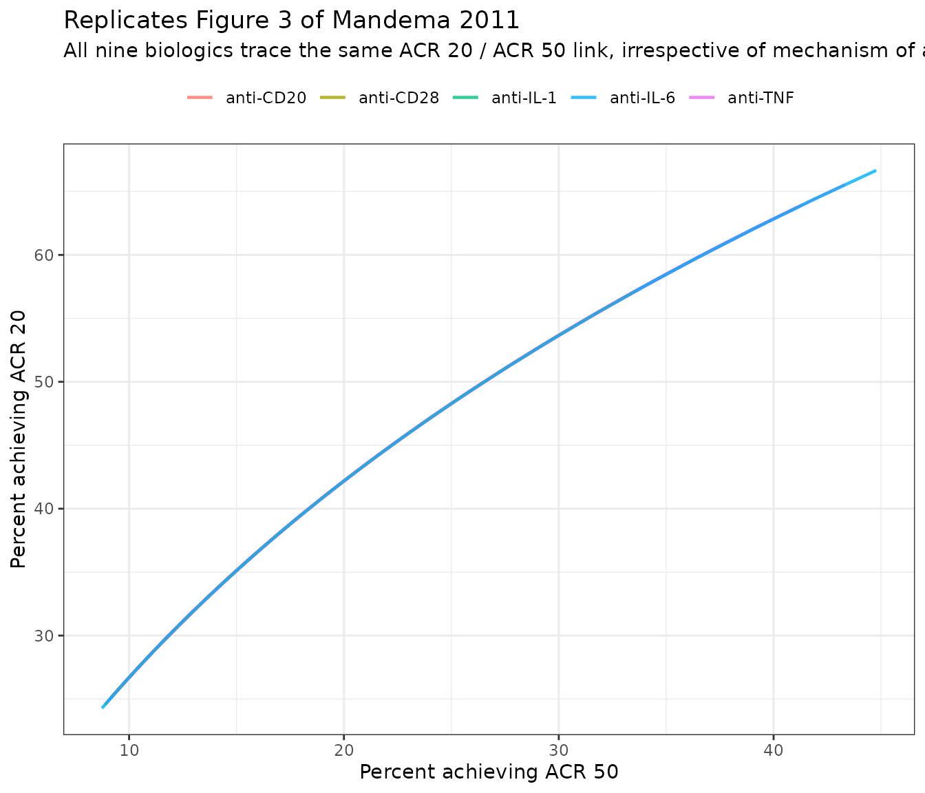
# Interpolate every drug's ACR 20 onto a common ACR 50 grid; the spread across
# drugs at a matched ACR 50 must be numerically zero. The grid spans the ACR 50
# range every drug actually reaches - anakinra's class Emax caps it well below
# the others, so a fixed grid would compare some drugs against nothing.
by_drug <- split(link, link$grid_drug)
p50_lo  <- max(vapply(by_drug, \(d) min(d$p_acr50), numeric(1)))
p50_hi  <- min(vapply(by_drug, \(d) max(d$p_acr50), numeric(1)))
stopifnot(p50_hi - p50_lo > 0.02)          # the common range must be real

p50_grid <- seq(p50_lo, p50_hi, length.out = 25)
link_mat <- vapply(by_drug, function(d) {
  d <- d[order(d$p_acr50), ]
  approx(d$p_acr50, d$p_acr20, xout = p50_grid)$y
}, numeric(length(p50_grid)))

stopifnot(!anyNA(link_mat))
# What is left is linear-interpolation error across the 60-point dose grid, not
# a difference between drugs: under 0.01 of a percentage point.
spread_link <- apply(link_mat, 1, \(x) diff(range(x)))
stopifnot(max(spread_link) < 5e-4)

cat("largest across-drug spread in ACR 20 at a matched ACR 50:",
    signif(100 * max(spread_link), 3), "percentage points\n")
#> largest across-drug spread in ACR 20 at a matched ACR 50: 0.00484 percentage points
Replicate Figure 4: the anti-TNFs collapse onto one curve
Figure 4 plots the anti-TNF dose-response against dose/ED50 rather than against dose, and the five drugs fall on a single line. That collapse is the visual form of the shared-Emax finding, and it is the property that makes the potency differences in Table 2 interpretable as a dosing choice rather than a molecular one.
collapse <- sim |>
  dplyr::filter(!is.na(grid_drug)) |>
  dplyr::mutate(class = ifelse(grid_moa == "anti-TNF", "anti-TNF", grid_moa))

ggplot(collapse, aes(dose_over_ed50, 100 * p_acr50,
                     colour = class, group = grid_drug)) +
  geom_line(linewidth = 0.7) +
  scale_x_log10(limits = c(0.05, 50)) +
  labs(x = "Dose / ED50", y = "Percent achieving ACR 50", colour = NULL,
       title = "Replicates Figure 4 of Mandema 2011",
       subtitle = paste("All five anti-TNFs superimpose; the other",
                        "mechanisms of action do not.")) +
  theme_bw() +
  theme(legend.position = "top")
#> Warning: Removed 56 rows containing missing values or values outside the scale range
#> (`geom_line()`).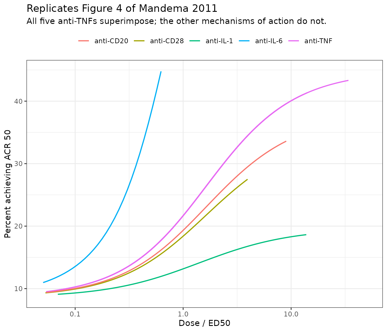
# On a common dose/ED50 grid the five anti-TNFs must agree to floating-point
# precision, and at least one other mechanism of action must not.
at_ratio <- function(drug, r) {
  ed50 <- get_arm(paste0("start:", drug))
  d <- table2$dose[table2$drug == drug] / ed50$dose_over_ed50 * r
  a <- make_arms("probe")
  a[[drug_table$column[drug_table$drug == drug]]] <- d
  a <- dplyr::mutate(dplyr::select(a, -"arm"), id = 1L)
  rxode2::rxSolve(mod, events = as.data.frame(a),
                  returnType = "data.frame")$p_acr50
}

tnf_at_2 <- vapply(tnf, at_ratio, numeric(1), r = 2)
stopifnot(diff(range(tnf_at_2)) < 1e-8)

# Tocilizumab at the same dose/ED50 must sit well above the anti-TNF curve,
# because its class Emax is larger.
stopifnot(at_ratio("tocilizumab", 2) > max(tnf_at_2) + 0.05)
The Discussion’s quantitative claims
The Discussion makes several arithmetic claims that the paper never tabulates. Each is an independent test of the recovered parameters.
probe <- function(drug, dose, naive = FALSE) {
  a <- make_arms("probe")
  a[[drug_table$column[drug_table$drug == drug]]] <- dose
  a <- dplyr::mutate(dplyr::select(a, -"arm"), id = 1L)
  s <- rxode2::rxSolve(mod, events = as.data.frame(a), returnType = "data.frame")
  if (naive) c(s$p_acr20_naive, s$p_acr50_naive, s$p_acr70_naive)
  else       c(s$p_acr20, s$p_acr50, s$p_acr70)
}

claims <- tibble::tibble(
  Claim = c(
    "Golimumab 100 mg q4w ~ adalimumab 40 mg q2w",
    "Golimumab 100 mg q4w ~ infliximab 3 mg/kg",
    "Adalimumab 80 mg q2w ~ etanercept 25 mg biw",
    "Infliximab 6 mg/kg ~ etanercept 25 mg biw",
    "Tocilizumab 8 mg/kg ~ etanercept 25 mg biw",
    "Tocilizumab 8 mg/kg ~ certolizumab 200 mg q2w"
  ),
  `ACR 20 gap (pp)` = 100 * c(
    probe("golimumab", 100)[1]  - probe("adalimumab", 40)[1],
    probe("golimumab", 100)[1]  - probe("infliximab", 3)[1],
    probe("adalimumab", 80)[1]  - probe("etanercept", 25)[1],
    probe("infliximab", 6)[1]   - probe("etanercept", 25)[1],
    probe("tocilizumab", 8)[1]  - probe("etanercept", 25)[1],
    probe("tocilizumab", 8)[1]  - probe("certolizumab", 200)[1]
  )
)

# "Comparable" / "similar" in the source means a few percentage points, not
# equality. The two golimumab claims are the tightest because both sides rest
# on the algebraically-recovered anti-TNF Emax; the tocilizumab claims are the
# loosest because tocilizumab's Emax is the figure-digitized one.
stopifnot(
  max(abs(claims$`ACR 20 gap (pp)`[1:2])) < 1.0,
  max(abs(claims$`ACR 20 gap (pp)`)) < 7.0
)

claims |>
  dplyr::mutate(`ACR 20 gap (pp)` = round(`ACR 20 gap (pp)`, 1)) |>
  knitr::kable(caption = paste0(
    "Discussion claims of comparable efficacy (Mandema 2011 p. 833). ",
    "A gap near zero confirms the claim."
))| Claim | ACR 20 gap (pp) |
|---|---|
| Golimumab 100 mg q4w ~ adalimumab 40 mg q2w | -0.3 |
| Golimumab 100 mg q4w ~ infliximab 3 mg/kg | 0.4 |
| Adalimumab 80 mg q2w ~ etanercept 25 mg biw | -2.2 |
| Infliximab 6 mg/kg ~ etanercept 25 mg biw | -2.6 |
| Tocilizumab 8 mg/kg ~ etanercept 25 mg biw | 5.6 |
| Tocilizumab 8 mg/kg ~ certolizumab 200 mg q2w | 2.3 |
An internal contradiction in the source
The Discussion states: “The differences are quite large, with golimumab having -10, -15, and -9% absolute difference values for ACR 20, 50, and 70 responses as compared with etanercept.” Table 2 gives those same three differences directly, by subtraction, and they are -15.8, -15.4 and -9.3. The ACR 50 and ACR 70 figures agree with the Discussion; the ACR 20 figure does not.
Table 2 has to be right, for a reason that does not depend on this model at all: the ACR 20 difference between two drugs cannot be smaller in magnitude than their ACR 50 difference, because the ACR 20 responder rate is uniformly higher and further from the floor. A -10 alongside a -15 is arithmetically impossible. The Discussion figure is a typesetting slip, most plausibly -16 set as -10.
gap_gol_eta <- 100 * (probe("golimumab", 50) - probe("etanercept", 25))

# Table 2, by subtraction: the arithmetic the Discussion sentence summarizes.
t2_gap <- as.numeric(
  table2[table2$drug == "golimumab",  c("acr20", "acr50", "acr70")] -
  table2[table2$drug == "etanercept", c("acr20", "acr50", "acr70")]
)

stopifnot(max(abs(gap_gol_eta - t2_gap)) < 0.2)

# The impossibility that identifies the Discussion's ACR 20 value as the error.
stopifnot(abs(t2_gap[1]) > abs(t2_gap[2]))

tibble::tibble(
  Endpoint = c("ACR 20", "ACR 50", "ACR 70"),
  `Table 2 (by subtraction)` = round(t2_gap, 1),
  `Discussion text` = c(-10, -15, -9),
  Simulated = round(gap_gol_eta, 1)
) |>
  knitr::kable(caption = paste0(
    "Golimumab 50 mg q4w minus etanercept 25 mg twice weekly, absolute ",
    "difference in ACR response (percentage points). The model follows ",
    "Table 2; the Discussion's ACR 20 value of -10 is inconsistent with it."
))| Endpoint | Table 2 (by subtraction) | Discussion text | Simulated |
|---|---|---|---|
| ACR 20 | -15.8 | -10 | -15.7 |
| ACR 50 | -15.4 | -15 | -15.4 |
| ACR 70 | -9.3 | -9 | -9.3 |
# "Doubling the dose of tocilizumab resulted in a much larger increase in ACR
# response as compared with doubling the dose of an anti-TNF because the shapes
# of the dose-response relationship curves differ depending on the mechanism of
# action." (Mandema 2011 p. 833)
doubling <- tibble::tibble(
  Drug = c("tocilizumab", "adalimumab", "etanercept", "infliximab",
           "golimumab", "certolizumab"),
  from = c(4, 40, 25, 3, 50, 200)
) |>
  dplyr::rowwise() |>
  dplyr::mutate(
    gain_pp = 100 * (probe(Drug, 2 * from)[1] - probe(Drug, from)[1])
  ) |>
  dplyr::ungroup()

toci_gain <- doubling$gain_pp[doubling$Drug == "tocilizumab"]
tnf_gain  <- doubling$gain_pp[doubling$Drug != "tocilizumab"]

# "Much larger" is not a number, so require a factor of at least two over the
# largest anti-TNF gain rather than mere ordering.
stopifnot(toci_gain > 2 * max(tnf_gain))

doubling |>
  dplyr::transmute(Drug,
                   `Starting dose` = from,
                   `ACR 20 gain on doubling (pp)` = round(gain_pp, 1)) |>
  knitr::kable(caption = paste0(
    "Gain in ACR 20 response from doubling the suggested starting dose. ",
    "Tocilizumab gains ", round(toci_gain / max(tnf_gain), 1),
    " times more than the best anti-TNF."
))| Drug | Starting dose | ACR 20 gain on doubling (pp) |
|---|---|---|
| tocilizumab | 4 | 16.9 |
| adalimumab | 40 | 5.7 |
| etanercept | 25 | 2.7 |
| infliximab | 3 | 5.9 |
| golimumab | 50 | 7.6 |
| certolizumab | 200 | 1.1 |
The East Asian trial effect
row_row  <- get_arm("asia:row")
asia_row <- get_arm("asia:eastasia")

# The effect is defined on the treatment effect (the log odds ratio versus the
# arm's own control), so that is where the 33% must appear exactly.
lor_ratio <- asia_row$lor_acr50 / row_row$lor_acr50
stopifnot(abs(lor_ratio - 1.33) < 1e-8)

tibble::tibble(
  Region = c("Rest of world", "East Asia"),
  `ACR 20 (%)` = round(100 * c(row_row$p_acr20, asia_row$p_acr20), 1),
  `ACR 50 (%)` = round(100 * c(row_row$p_acr50, asia_row$p_acr50), 1),
  `ACR 70 (%)` = round(100 * c(row_row$p_acr70, asia_row$p_acr70), 1),
  `ACR 50 log odds ratio` = round(c(row_row$lor_acr50, asia_row$lor_acr50), 3)
) |>
  knitr::kable(caption = paste0(
    "Etanercept 25 mg twice weekly, with and without the East Asian trial ",
    "indicator. The log odds ratio is exactly ", round(lor_ratio, 2),
    " times larger, matching the published 33% (95% CI 12 to 54%)."
))| Region | ACR 20 (%) | ACR 50 (%) | ACR 70 (%) | ACR 50 log odds ratio |
|---|---|---|---|---|
| Rest of world | 61.1 | 37.9 | 18.2 | 1.870 |
| East Asia | 72.7 | 53.1 | 30.7 | 2.487 |
No PKNCA validation
PKNCA validation does not apply to this model. There is no PK layer, no concentration-time profile and no dosing event to integrate: the model maps a per-arm dose directly onto a per-arm responder probability at a single unspecified time point. The validation above is instead a full replication of the source’s four results tables and two of its figures, which is the analogue of an NCA check for a dose-response meta-analysis.
Assumptions and deviations
No parameter table exists in the source. Only two numeric parameters are printed anywhere in Mandema 2011 or its supplement: the combination-therapy interaction coefficient (-0.32) and the East Asian effect (33%). Every other value in
ini()was recovered by inverting Tables 2-4, the Discussion dose/ED50 ratios and the Figure 2 curves, as set out in “Recovering the unpublished parameters” above. The recovery is over-determined at three separate points (four ratios implying one anti-TNF Emax to 1.2%; nine drugs implying one pair of endpoint scale factors to 0.5%; five Table 3 rows implying one MTX-naive placebo response per endpoint to 0.1 percentage points), and it predicts Table 4 out of sample to under a percentage point. It is nonetheless a reconstruction, and a reader who obtains the authors’ original estimates should prefer them.Figure-digitized values.
emax_antiil1,emax_cd28,emax_cd20andemax_antiil6were read off Figure 2 rather than from any printed number, because anakinra, abatacept, rituximab and tocilizumab are each the only member of their mechanism-of-action class and Table 2 gives one equation in two unknowns for each. The measured digitization bias, from applying the same procedure to the five anti-TNF panels whose Emax is known algebraically, is +2.2%. The matching ED50 values are not digitized: each is set so that the digitized Emax reproduces the published Table 2 point exactly.Endpoint scaling: Table 2 over the prose. The Results state that the treatment effect is “11% (6.2 to 17%) smaller (relative decrease) for ACR 20 as compared with ACR 50, and 11% (2.1 to 19%) larger for ACR 70 as compared with ACR 50.” The 27 cells of Table 2 give 14.3% and 11.3%. Both Table 2 values sit inside the published confidence intervals, and Table 2 is used here because it is the more precise statement of the same quantity and because it also regenerates Tables 3 and 4. Using the prose values instead would move the predicted Table 2 ACR 20 column by about one percentage point in each row.
Erratum: the Discussion’s golimumab-versus-etanercept ACR 20 difference is wrong. The text gives “-10, -15, and -9%” for ACR 20, 50 and 70; Table 2 gives -15.8, -15.4 and -9.3 by subtraction. Only the ACR 20 value disagrees, and it disagrees in a direction that is arithmetically impossible: a between-drug difference cannot shrink when moving from ACR 50 to the uniformly higher ACR 20 responder rate. The model follows Table 2. This is recorded here rather than silently reconciled because a reader checking the model against the Discussion sentence would otherwise think the model wrong.
The combination interaction is formed after the endpoint scaling. The printed equation is written on , the endpoint-specific effect, which implies the product term is formed per endpoint. The alternative reading - form the product on the ACR 50 scale and scale the result - is not excluded by the typography, but it misses the published Table 4 ACR 20 column by up to 2.1 percentage points where the reading used here lands within 0.5. Monotherapy arms are identical under both readings.
Emax is indexed by endpoint even though the printed equation is not. The typeset dose-response equation writes without a
ksubscript, but the function it defines is and the surrounding text describes retaining an endpoint difference in Emax and rejecting one in ED50. The constancy of the per-drug ratio across nine drugs spanning a 50-fold range of dose/ED50 confirms the Emax reading empirically; an ED50 difference would make that ratio vary with dose.The MTX-naive population is carried as a second set of intercepts, not as a covariate. The source found “no statistically significant difference in the odds ratio (relative to placebo) for MTX-naive patients vs. patients who had shown inadequate response to prior MTX treatment”, so the two populations differ only in their placebo response. Both sets of outputs (
p_acr*andp_acr*_naive) are therefore returned from every solve and the treatment effect is shared. Thelor_acr*outputs are population-independent and are the quantities the source actually identified.No random effects and no residual error. Between-trial random effects on Emax and ED50 were tested and rejected by the source. The one random effect it retained, on the ACR 20 and ACR 70 placebo responses, has a variance that is not reported anywhere; per the unreported-variance convention it is omitted rather than invented. Observed placebo responses ranged from 8.7 to 42% (ACR 20), 0 to 29% (ACR 50) and 0 to 16% (ACR 70) across the 50 trials; a user reproducing a specific trial should shift
e0_acr50rather than add a random effect, which the source licenses by finding no effect of the placebo-response magnitude on the treatment effect. The likelihood was binomial on per-arm counts, so a user who wants simulated counts should drawrbinom(1, size = N_arm, prob = p_acr50)downstream.One drug per arm. Every trial arm in the source received at most one biologic. Setting two biologic dose columns non-zero simultaneously makes the model add their effects, which is outside the source’s calibration.
The MTX dose column carries presence, not magnitude.
CONMED_MTX_DOSEactivates a mean effect whenever it is non-zero, because the source estimated no MTX dose-response (“MTX was titrated to a similar dose range in all the trials and no dose-response data were available”). Values outside the titrated 15-20 mg/week range are outside the calibration.The East Asian effect is applied to the biologic term only. It is defined on Emax, and randomized MTX has no Emax. Four of the 50 trials were East Asian (three in Japan, one in Taiwan).
Anakinra’s class Emax is much smaller than the anti-TNFs’. The recovered value (0.954 versus 2.157) reflects the paper’s finding that “of all the biologics, anakinra provided the smallest treatment effect”, but the source also reports the Emax difference between anakinra and the anti-TNFs as not statistically significant. With three anakinra trials over a narrow effective dose range that is unsurprising; the point estimate should be read as imprecise.