Anticoagulant therapeutic index for VTE prophylaxis (Mandema 2011) • nlmixr2lib

Model and source

Citation: Mandema JW, Boyd RA, DiCarlo LA. Therapeutic index of anticoagulants for prevention of venous thromboembolism following orthopedic surgery: a dose-response meta-analysis. Clin Pharmacol Ther. 2011;90(6):820-827. doi:10.1038/clpt.2011.232. Dose-response equations and all parameter estimates are in the Supplementary Data section ‘Parameter estimates [95% CI] of the joint analysis of all efficacy and bleeding endpoints’.
Article: https://doi.org/10.1038/clpt.2011.232
Supplement: linked from the article landing page; it carries the trial-level data table, the two dose-response equations, and the full parameter table used below.

This is a model-based meta-analysis (MBMA), not a population PK model. It has no PK layer, no ODE states, no between-subject variability and no residual error model. The unit of prediction is a study arm, and the outputs are per-arm event probabilities.

Population

Mandema and colleagues pooled 89 randomized controlled trials of venous thromboembolism (VTE) prophylaxis after elective total hip replacement (THR) or total knee replacement (TKR) surgery, covering 92,543 patients and 23 anticoagulants across seven drug classes. 87 trials contributed efficacy data and 74 contributed bleeding data; 15 trials (1,286 patients) were placebo-controlled and enoxaparin was the active control in 39% of trials. Trials were required to enroll at least 75% hip- or knee-replacement patients and to use mandatory end-of-period venography for VTE ascertainment. Per-drug trial counts, patient counts, daily-dose ranges and regional distribution are in Mandema 2011 Table 1; per-arm mean age, percent hip surgery and event counts are in the supplement’s trial-overview table.

Three efficacy endpoints were modelled jointly (clinical pulmonary embolism; major VTE, i.e. proximal DVT + clinical PE +/- death; and total VTE, i.e. distal DVT + major VTE) and three bleeding endpoints (major bleeding by ISTH criteria adapted for surgery; major + clinically-relevant-non-major (CRNM) bleeding; and total bleeding).

The same information is available programmatically from the model’s population metadata (readModelDb("Mandema_2011_anticoagulants_mbma")()$population - readModelDb() returns the model function, so the trailing () evaluates it).

Model structure

Per-arm event counts were assumed binomial, and the probability of an event for endpoint k in arm j of trial i was modelled on the logit scale as an intercept plus a dose-response term (Mandema 2011 Methods):

N_event,kij ~ binomial(P(event)kij, N_kij)
P(event)kij = f{ E0,ki -/+ g(Drug_ij, Dose_ij, X_ij, theta_i)_k }

where f is the inverse logit. E0,ki is a separate nuisance intercept for each of the 89 trials, which is why the source states that “the primary response variable is the log of the odds ratio between the active and the control arms”. The efficacy term is subtracted (dose reduces VTE risk); the bleeding term is added (dose increases bleeding risk, as Figures 2 and 3 show).

The two dose-response functions are given in the supplement:

                    (Emax + Emax,endpoint) * Dose^n
g_efficacy = --------------------------------------------------------
             Dose^n + (ED50,drug * ED50,endpoint * ED50,class,endpoint)^n

                     Dose
g_bleeding = ------------------------- * (1 + Sc_bld,endpoint)
             ED50,drug * EDbld,class

Three structural points drive everything downstream:

Each drug has its own ED50 for major VTE, and clinical PE reuses the major-VTE Emax and ED50 exactly (“A separate ED50 or Emax could not be estimated for PE … A model that assumed that the Emax and ED50 values for PE were the same as those for major VTE for each drug best described the PE data”). PE and major VTE therefore differ only in their intercept.
The total-VTE potency shift is a drug-CLASS property, not a drug property - the finding that “the difference in drug potency for major VTE vs. total VTE is dependent on the mechanism of action only”.
EDbld is parameterised as a ratio to the drug’s own major-VTE ED50, and that ratio is a class property. Because the relative therapeutic index is (EDbld / ED50,vte)_drug / (EDbld / ED50,vte)_enoxaparin, the ED50,drug cancels and the relative TI reduces to a ratio of class parameters. That is exactly why the source finds “significant differences in the therapeutic index … across the drug classes but not for drugs within a class”.

No covariate was retained: “None of the covariates significantly influenced the ED50 or Emax” and “None of the covariates significantly impacted the slope of the bleeding dose-response relationship”. Trial-level random effects on Emax and ED50 were tested and rejected. The screened-but-dropped covariates are recorded in the model’s covariatesDataExcluded metadata.

Source trace

Every ini() value carries an in-file comment pointing at its source. The table below collects them.

Equation / parameter	Value	Source location
Binomial likelihood, logit link, per-trial intercept	n/a	Mandema 2011 Methods, “analysis methodology”
Sigmoid Emax efficacy dose-response	n/a	Mandema 2011 Results “Efficacy” equation; supplement equation 1
Linear bleeding dose-response	n/a	Mandema 2011 Results “Bleeding” equation; supplement equation 2
`emax`	3.18	Supplement parameter table, `Emax` [2.59 to 3.76]
`emax_totalvte`	-0.744	Supplement parameter table, `EmaxtotalVTE` [-1.18 to -0.303]
`lhill`	log(1.33)	Supplement parameter table, `n` [1.09 to 1.61]
`led50_enoxaparin`	log(61.6) mg/day	Supplement, `ED50 Enoxaparin` [44.9 to 84.5]
`led50_ardeparin`	log(101) IU/kg/day	Supplement, `ED50 Ardeparin` [66.6 to 154]
`led50_bemiparin`	log(3.62) kIU/day	Supplement, `ED50 Bemiparin` [2.12 to 6.18]
`led50_dalteparin`	log(5.57) kIU/day	Supplement, `ED50 Dalteparin` [3.81 to 8.14]
`led50_nadroparin`	log(78.4) IU/kg/day	Supplement, `ED50 Nadroparin` [50.1 to 123]
`led50_reviparin`	log(6.29) kIU/day	Supplement, `ED50 Reviparin` [4.07 to 9.72]
`led50_tinzaparin`	log(105) IU/kg/day	Supplement, `ED50 Tinzaparin` [69.9 to 158]
`led50_apixaban`	log(4.31) mg/day	Supplement, `ED50 Apixaban` [2.85 to 6.51]
`led50_betrixaban`	log(214) mg/day	Supplement, `ED50 Betrixaban` [41.6 to 1100]
`led50_edoxaban`	log(15.2) mg/day	Supplement, `ED50 Edoxaban` [8.78 to 26.3]
`led50_razaxaban`	log(18.1) mg/day	Supplement, `ED50 Razaxaban` [8.94 to 36.5]
`led50_rivaroxaban`	log(5.51) mg/day	Supplement, `ED50 Rivaroxaban` [3.6 to 8.44]
`led50_ly517717`	log(225) mg/day	Supplement, `ED50 LY517717` [94.9 to 534]
`led50_pd0348292`	log(1.98) mg/day	Supplement, `ED50 Pd0348292` [1.07 to 3.66]
`led50_ym150`	log(26.1) mg/day	Supplement, `ED50 YM150` [8.95 to 76.3]
`led50_ave5026`	log(13.1) mg/day	Supplement, `ED50 AVE5026` [7.49 to 23]
`led50_fondaparinux`	log(1.97) mg/day	Supplement, `ED50 Fondaparinux` [1.22 to 3.19]
`led50_dabigatran`	log(229) mg/day	Supplement, `ED50 dabigatran` [159 to 330]
`led50_ximelagatran`	log(78.8) mg/day	Supplement, `ED50 Ximelagatran` [54.3 to 114]
`led50_desirudin`	log(21.4) mg/day	Supplement, `ED50 Desirudin` [13.5 to 33.8]
`led50_sr123781a`	log(1.41) mg/day	Supplement, `ED50 SR123781A` [0.397 to 4.99]
`led50_heparin`	log(57.9) kIU/day	Supplement, `ED50 Heparin` [28.5 to 118]
`led50_warfarin`	log(4.05) INR	Supplement, `ED50 Warfarin (INR)` [2.71 to 6.04]
`ratio_ed50_ximelagatran_presurg`	0.365	Supplement, `ED50 Ximelagatran started before surgery / ED50 Ximelagatran` [0.286 to 0.466]
`ratio_ed50_totalvte`	0.721	Supplement, `ED50,totalVTE` [0.549 to 0.947]
`ratio_ed50_totalvte_lmwh`	1.26	Supplement, `ED50,totalVTE LMWH other than enoxaparin` [1.04 to 1.52]
`ratio_ed50_totalvte_dfxa`	0.769	Supplement, `ED50,totalVTE direct FXa inhibitor` [0.621 to 0.953]
`ratio_ed50_totalvte_ifxa`	0.499	Supplement, `ED50,totalVTE indirect FXa inhibitor` [0.331 to 0.752]
`ratio_ed50_totalvte_uthr`	1.28	Supplement, `ED50,totalVTE univalent thrombin inhibitor` [1.1 to 1.48]
`ratio_ed50_totalvte_bthr`	1.03	Supplement, `ED50,totalVTE bivalent thrombin inhibitor` [0.744 to 1.44]
`ratio_ed50_totalvte_mixed`	1.97	Supplement, `ED50,totalVTE mixed FXa and thrombin inhibitors` [0.626 to 6.2]
`ratio_ed50_totalvte_heparin`	0.535	Supplement, `ED50,totalVTE Heparin` [0.332 to 0.864]
`ratio_ed50_totalvte_warfarin`	1.7	Supplement, `ED50,totalVTE Warfarin` [1.34 to 2.15]
`ratio_edbld_enox`	1.7	Supplement, `EDbldEnoxaparin` [1.14 to 2.54]
`ratio_edbld_lmwh`	1.58	Supplement, `EDbld LMWH other than enoxaparin` [0.923 to 2.71]
`ratio_edbld_dfxa`	3.98	Supplement, `EDbld direct FXa inhibitor` [2.51 to 6.29]
`ratio_edbld_ifxa`	1.28	Supplement, `EDbld indirect FXa inhibitor` [0.762 to 2.16]
`ratio_edbld_uthr`	1.43	Supplement, `EDbld univalent thrombin inhibitor` [0.943 to 2.16]
`ratio_edbld_bthr`	3.72	Supplement, `EDbld bivalent thrombin inhibitor` [0.652 to 21.3]
`ratio_edbld_mixed`	0.841	Supplement, `EDbld mixed FXa and thrombin inhibitors` [0.231 to 3.07]
`ratio_edbld_heparin`	0.312	Supplement, `EDbld Heparin` [0.142 to 0.687]
`sc_bld_crnm`	-0.291	Supplement, `Scbld,CRNM+major` [-0.501 to -0.0804]
`sc_bld_total`	-0.369	Supplement, `Scbld,total bleed` [-0.494 to -0.243]
`e0_pe`	-4.768	Figure 1, PE panel - digitized (see Assumptions)
`e0_majorvte`	-1.964	Figure 1, major VTE panel - digitized
`e0_totalvte`	-0.644	Figure 1, VTE panel - digitized
`e0_majorbld`	-4.976	Figure 2, major bleeding panel - digitized
`e0_crnmbld`	-3.579	Figure 2, major + CRNM bleeding panel - digitized
`e0_totalbld`	-2.953	Figure 2, total bleeding panel - digitized
Reference levels (enoxaparin class ratio = 1; major-bleeding `Sc` = 0)	n/a	Definitional; the supplement tabulates only non-reference levels
No random effects	n/a	Mandema 2011 Results: trial-specific random effects on Emax/ED50 “did not result in a significant improvement of fit”

Virtual cohort

There is no subject-level cohort to simulate: the model predicts study-arm outcomes. The “cohort” here is therefore a grid of study arms - one row per (drug, daily dose) combination - built over the daily-dose ranges the source actually studied (Mandema 2011 Table 1).

set.seed(20261101)

covariate_names <- c(
  "CONMED_ENOXAPARIN_DOSE", "CONMED_ARDEPARIN_DOSE", "CONMED_BEMIPARIN_DOSE",
  "CONMED_DALTEPARIN_DOSE", "CONMED_NADROPARIN_DOSE", "CONMED_REVIPARIN_DOSE",
  "CONMED_TINZAPARIN_DOSE", "CONMED_APIXABAN_DOSE", "CONMED_BETRIXABAN_DOSE",
  "CONMED_EDOXABAN_DOSE", "CONMED_RAZAXABAN_DOSE", "CONMED_RIVAROXABAN_DOSE",
  "CONMED_LY517717_DOSE", "CONMED_PD0348292_DOSE", "CONMED_YM150_DOSE",
  "CONMED_AVE5026_DOSE", "CONMED_FONDAPARINUX_DOSE", "CONMED_DABIGATRAN_DOSE",
  "CONMED_XIMELAGATRAN_DOSE", "CONMED_DESIRUDIN_DOSE", "CONMED_SR123781A_DOSE",
  "CONMED_HEPARIN_DOSE", "CONMED_WARFARIN_DOSE", "FORM_XIMELAGATRAN_PRESURG"
)

# Drug -> (dose column, drug class, studied daily-dose range) from Table 1.
drug_table <- tibble::tribble(
  ~drug,            ~column,                    ~drug_class,             ~dose_lo, ~dose_hi,
  "enoxaparin",     "CONMED_ENOXAPARIN_DOSE",   "enoxaparin",                  10,       60,
  "ardeparin",      "CONMED_ARDEPARIN_DOSE",    "LMWH (other)",                50,      100,
  "bemiparin",      "CONMED_BEMIPARIN_DOSE",    "LMWH (other)",               3.5,      3.5,
  "dalteparin",     "CONMED_DALTEPARIN_DOSE",   "LMWH (other)",                 5,        5,
  "nadroparin",     "CONMED_NADROPARIN_DOSE",   "LMWH (other)",                43,       60,
  "reviparin",      "CONMED_REVIPARIN_DOSE",    "LMWH (other)",               2.8,      4.2,
  "tinzaparin",     "CONMED_TINZAPARIN_DOSE",   "LMWH (other)",                50,       75,
  "apixaban",       "CONMED_APIXABAN_DOSE",     "direct FXa inhibitor",         5,       20,
  "betrixaban",     "CONMED_BETRIXABAN_DOSE",   "direct FXa inhibitor",        30,       80,
  "edoxaban",       "CONMED_EDOXABAN_DOSE",     "direct FXa inhibitor",         5,       90,
  "razaxaban",      "CONMED_RAZAXABAN_DOSE",    "direct FXa inhibitor",        50,      200,
  "rivaroxaban",    "CONMED_RIVAROXABAN_DOSE",  "direct FXa inhibitor",         5,       60,
  "LY517717",       "CONMED_LY517717_DOSE",     "direct FXa inhibitor",        25,      150,
  "PD0348292",      "CONMED_PD0348292_DOSE",    "direct FXa inhibitor",       0.1,       10,
  "YM150",          "CONMED_YM150_DOSE",        "direct FXa inhibitor",         3,       60,
  "AVE5026",        "CONMED_AVE5026_DOSE",      "direct FXa inhibitor",         5,       60,
  "fondaparinux",   "CONMED_FONDAPARINUX_DOSE", "indirect FXa inhibitor",     0.8,        8,
  "dabigatran",     "CONMED_DABIGATRAN_DOSE",   "univalent thrombin inh.",     25,      600,
  "ximelagatran",   "CONMED_XIMELAGATRAN_DOSE", "univalent thrombin inh.",     12,       72,
  "desirudin",      "CONMED_DESIRUDIN_DOSE",    "bivalent thrombin inh.",      20,       40,
  "SR123781A",      "CONMED_SR123781A_DOSE",    "mixed FXa/thrombin inh.",    0.2,        4,
  "heparin",        "CONMED_HEPARIN_DOSE",      "heparin",                     10,       15,
  "warfarin",       "CONMED_WARFARIN_DOSE",     "warfarin",                   2.2,      2.5
)

# Build study arms: every covariate column is 0 except the one drug being given.
make_arms <- function(drug_name, doses, presurg = 0, id_offset = 0L) {
  info <- drug_table[drug_table$drug == drug_name, ]
  stopifnot(nrow(info) == 1)
  zeros <- as.list(rep(0, length(covariate_names)))
  names(zeros) <- covariate_names
  out <- tibble::as_tibble(zeros)[rep(1, length(doses)), ]
  out[[info$column]] <- doses
  out$FORM_XIMELAGATRAN_PRESURG <- presurg
  dplyr::bind_cols(
    tibble::tibble(
      id         = id_offset + seq_along(doses),
      time       = 0,
      evid       = 0,
      drug       = drug_name,
      drug_class = info$drug_class,
      dose       = doses
    ),
    out
  )
}

# A placebo arm (every dose column 0) plus each drug over its studied range.
placebo_arm <- make_arms("enoxaparin", 0, id_offset = 0L)
placebo_arm$drug <- "placebo"
placebo_arm$drug_class <- "placebo"

n_per_drug <- 60L  # dose grid points per drug arm; each "subject" is a study arm
arms <- list(placebo_arm)
offset <- 1L
for (d in drug_table$drug) {
  info <- drug_table[drug_table$drug == d, ]
  # Bemiparin and dalteparin were each studied at a single daily dose, which
  # would make a log-spaced grid degenerate; widen those to a 20-fold span so
  # the figures show a curve. This affects the plotted range only.
  lo <- if (isTRUE(all.equal(info$dose_lo, info$dose_hi))) {
    info$dose_hi / 20
  } else {
    info$dose_lo
  }
  grid <- exp(seq(log(lo), log(info$dose_hi), length.out = n_per_drug))
  arms[[length(arms) + 1L]] <- make_arms(d, grid, id_offset = offset)
  offset <- offset + n_per_drug
}
arms <- dplyr::bind_rows(arms)

stopifnot(!anyDuplicated(arms$id))
cat("study arms simulated:", nrow(arms), "over", length(unique(arms$drug)), "arm labels\n")
#> study arms simulated: 1381 over 24 arm labels

Simulation

mod <- readModelDb("Mandema_2011_anticoagulants_mbma")

sim <- rxode2::rxSolve(
  mod,
  events = as.data.frame(arms),
  keep = unname(c("drug", "drug_class", "dose")),
  returnType = "data.frame"
) |>
  tibble::as_tibble()

# The model is deterministic: no etas, no residual error. One row per arm.
stopifnot(nrow(sim) == nrow(arms))

Placebo arm reproduces the intercepts

A placebo arm sets every dose column to 0, which collapses both dose-response terms to zero and leaves the per-endpoint intercept. This is an exact check.

plc <- sim |> dplyr::filter(drug == "placebo")
ilogit <- function(x) 1 / (1 + exp(-x))

e0 <- c(pe = -4.768, majorvte = -1.964, totalvte = -0.644,
        majorbld = -4.976, crnmbld = -3.579, totalbld = -2.953)

placebo_check <- tibble::tibble(
  endpoint  = names(e0),
  simulated = c(plc$p_pe, plc$p_majorvte, plc$p_totalvte,
                plc$p_majorbld, plc$p_crnmbld, plc$p_totalbld),
  expected  = ilogit(e0)
)

# Exact: the two sides are the same closed form evaluated at dose 0, so the
# only difference possible is floating-point noise.
stopifnot(max(abs(placebo_check$simulated - placebo_check$expected)) < 1e-12)

placebo_check |>
  dplyr::mutate(`Incidence (%)` = round(100 * simulated, 2)) |>
  dplyr::select("Endpoint" = endpoint, "Incidence (%)") |>
  knitr::kable(caption = "Control-arm (placebo) event incidence implied by the model intercepts.")

Control-arm (placebo) event incidence implied by the model intercepts.
Endpoint	Incidence (%)
pe	0.84
majorvte	12.30
totalvte	34.43
majorbld	0.69
crnmbld	2.71
totalbld	4.96

Replicate Figure 1: efficacy dose-response

Figure 1 plots incidence against the enoxaparin-equivalent dose - “the dose of the drug multiplied by the ratio of the ED50 of enoxaparin and the ED50 of the drug” - and shows that, because the drugs differ only in potency, they all lie on the enoxaparin curve once potency is accounted for. The model emits that x-axis directly as dose_enox_equiv.

efficacy_long <- sim |>
  dplyr::filter(drug != "placebo") |>
  dplyr::select(drug, drug_class, dose_enox_equiv,
                `total VTE` = p_totalvte, `major VTE` = p_majorvte, `PE` = p_pe) |>
  tidyr::pivot_longer(c(`total VTE`, `major VTE`, `PE`),
                      names_to = "endpoint", values_to = "p") |>
  dplyr::mutate(endpoint = factor(endpoint, levels = c("total VTE", "major VTE", "PE")))

ggplot(efficacy_long, aes(dose_enox_equiv, 100 * p, colour = drug_class)) +
  geom_line(aes(group = drug), linewidth = 0.6) +
  facet_wrap(~endpoint, scales = "free_y") +
  scale_x_log10() +
  labs(x = "Enoxaparin-equivalent dose (mg/day)", y = "Incidence (%)",
       colour = "Drug class",
       title = "Figure 1 - anticoagulant dose vs. response by efficacy endpoint",
       caption = "Replicates Figure 1 of Mandema 2011.") +
  theme(legend.position = "bottom")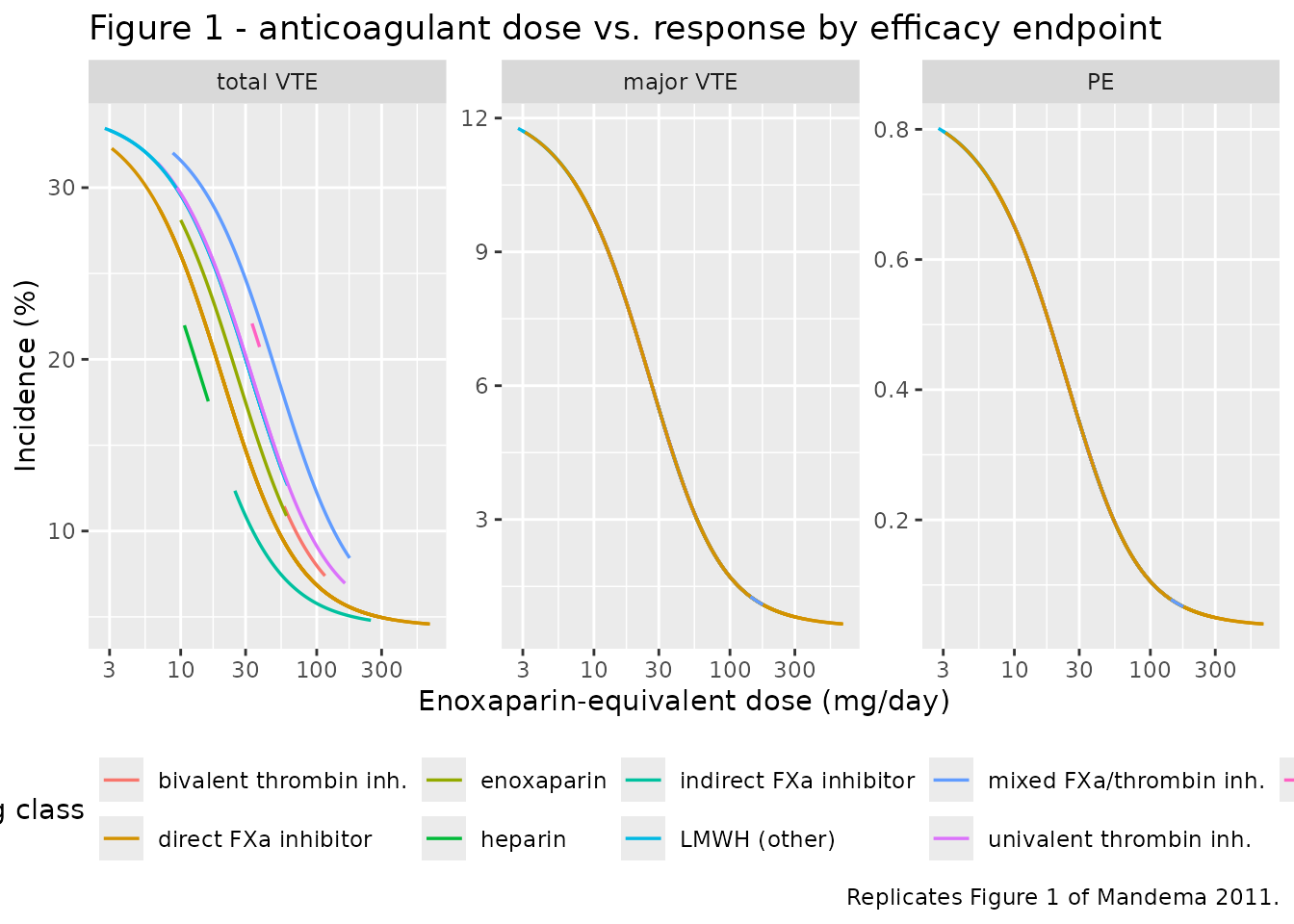

Hard gate - the potency collapse. For major VTE and PE, Emax and ED50 are shared across drugs, so every drug must land on exactly the same curve when plotted against enoxaparin-equivalent dose. For total VTE they must separate by class, which is the paper’s drug-class interaction finding.

# Predicted enoxaparin curve, evaluated at each arm's enoxaparin-equivalent dose.
emax <- 3.18; emax_tv <- -0.744; hill <- 1.33; ed50_enox <- 61.6
enox_majorvte <- function(d) {
  u <- (d / ed50_enox)^hill
  ilogit(e0[["majorvte"]] - emax * u / (u + 1))
}

collapse <- sim |>
  dplyr::filter(drug != "placebo") |>
  dplyr::mutate(expected = enox_majorvte(dose_enox_equiv),
                dev = abs(p_majorvte - expected))

# Every one of the 23 drugs collapses onto the enoxaparin major-VTE curve.
stopifnot(max(collapse$dev) < 1e-12)

# Total VTE must NOT collapse: the class ratios separate the curves. Compare
# each class against enoxaparin at a common enoxaparin-equivalent dose of 40.
class_at_40 <- sim |>
  dplyr::filter(drug != "placebo", dplyr::between(dose_enox_equiv, 39.5, 40.5)) |>
  dplyr::group_by(drug_class) |>
  dplyr::summarise(p = mean(p_totalvte), .groups = "drop")
# At least a 2 percentage-point spread across classes at a matched equivalent dose.
stopifnot(diff(range(100 * class_at_40$p)) > 2)

cat("max deviation from the enoxaparin major-VTE curve:",
    format(max(collapse$dev), digits = 3), "\n")
#> max deviation from the enoxaparin major-VTE curve: 5.55e-17
cat("total-VTE incidence across classes at 40 mg/day enoxaparin-equivalent: ",
    paste(sprintf("%s %.1f%%", class_at_40$drug_class, 100 * class_at_40$p),
          collapse = "; "), "\n")
#> total-VTE incidence across classes at 40 mg/day enoxaparin-equivalent:  LMWH (other) 16.9%; direct FXa inhibitor 12.0%; enoxaparin 14.4%; indirect FXa inhibitor 9.0%; mixed FXa/thrombin inh. 21.7%; univalent thrombin inh. 17.0%

Replicate Figure 2: bleeding dose-response

bleeding_long <- sim |>
  dplyr::filter(drug != "placebo", drug != "warfarin") |>
  dplyr::select(drug, drug_class, dose_enox_equiv,
                `major bleeding` = p_majorbld,
                `major + CRNM bleeding` = p_crnmbld,
                `total bleeding` = p_totalbld) |>
  tidyr::pivot_longer(-c(drug, drug_class, dose_enox_equiv),
                      names_to = "endpoint", values_to = "p") |>
  dplyr::mutate(endpoint = factor(endpoint,
    levels = c("major bleeding", "major + CRNM bleeding", "total bleeding")))

ggplot(bleeding_long, aes(dose_enox_equiv, 100 * p, colour = drug_class)) +
  geom_line(aes(group = drug), linewidth = 0.6) +
  facet_wrap(~endpoint, scales = "free_y") +
  scale_x_log10() +
  labs(x = "Enoxaparin-equivalent dose (mg/day)", y = "Incidence (%)",
       colour = "Drug class",
       title = "Figure 2 - anticoagulant dose vs. response by bleeding endpoint",
       caption = paste("Replicates Figure 2 of Mandema 2011.",
                       "Warfarin is omitted: no EDbld was estimable for it.")) +
  theme(legend.position = "bottom")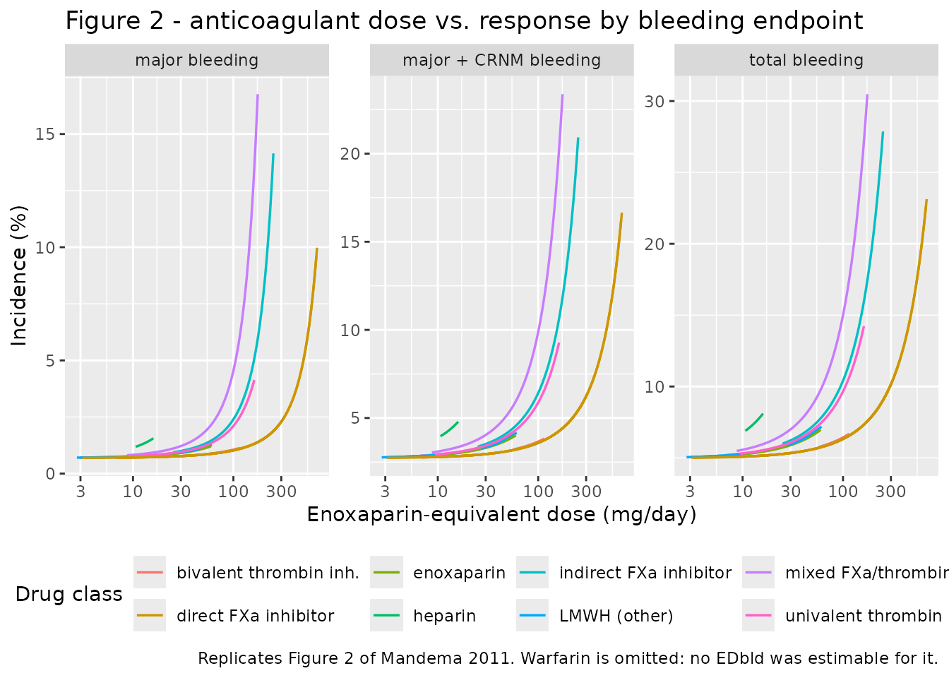

Hard gate - bleeding rises with dose, and the three endpoints are ordered. The source states that bleeding risk shows “the steep inflection point for increased bleeding risk if the dose increases above the equivalent of 100 mg/day enoxaparin”, and that “the slope of the dose-response relationship for total bleeding was smaller than that for major bleeding”. Both are checked directly.

enox_curve <- sim |>
  dplyr::filter(drug == "enoxaparin") |>
  dplyr::arrange(dose)

# 1. Bleeding is strictly increasing in dose for all three endpoints.
stopifnot(all(diff(enox_curve$p_majorbld) > 0),
          all(diff(enox_curve$p_crnmbld)  > 0),
          all(diff(enox_curve$p_totalbld) > 0))

# 2. Efficacy is strictly decreasing in dose for all three endpoints.
stopifnot(all(diff(enox_curve$p_pe)       < 0),
          all(diff(enox_curve$p_majorvte) < 0),
          all(diff(enox_curve$p_totalvte) < 0))

# 3. Slope ordering on the log-odds scale: total bleeding shallower than major.
slope <- function(lor, dose) stats::coef(stats::lm(lor ~ dose))[["dose"]]
s_major <- slope(enox_curve$lor_majorbld, enox_curve$dose)
s_crnm  <- slope(enox_curve$lor_crnmbld,  enox_curve$dose)
s_total <- slope(enox_curve$lor_totalbld, enox_curve$dose)
stopifnot(s_total < s_crnm, s_crnm < s_major)

# The scalars are exactly the published (1 + Sc) factors.
stopifnot(abs(s_crnm  / s_major - (1 - 0.291)) < 1e-10,
          abs(s_total / s_major - (1 - 0.369)) < 1e-10)

cat(sprintf("bleeding log-odds slope ratios vs major bleeding: CRNM+major %.3f, total %.3f\n",
            s_crnm / s_major, s_total / s_major))
#> bleeding log-odds slope ratios vs major bleeding: CRNM+major 0.709, total 0.631

Replicate Table 2: relative therapeutic index by drug class

Table 2 gives the relative TI for major bleeding vs. major VTE for every pairwise comparison of drug classes. The model-derived TI for a class is recovered end-to-end from the simulation, not by re-reading the parameters: for a representative drug of each class we find (a) the dose at which the major-VTE effect reaches half of Emax, and (b) the dose at which the major-bleeding log odds ratio reaches 1 - which is precisely the source’s definition, “EDbld represents the dose that yields a change of one in the log of the odds ratio”. Their ratio is the drug’s TI, and the relative TI is the ratio of two such.

representative <- c(
  "Enoxaparin"                 = "enoxaparin",
  "LMWH"                       = "dalteparin",
  "Direct FXa inhibitors"      = "rivaroxaban",
  "Indirect FXa inhibitors"    = "fondaparinux",
  "Direct thrombin inhibitors" = "dabigatran",
  "Heparin"                    = "heparin"
)

# Simulate each representative drug over a wide dose grid so both roots are
# bracketed, then invert numerically.
ti_from_simulation <- function(drug_name) {
  info <- drug_table[drug_table$drug == drug_name, ]
  grid <- exp(seq(log(info$dose_hi / 5000), log(info$dose_hi * 500), length.out = 4000))
  ev <- make_arms(drug_name, grid)
  s <- rxode2::rxSolve(mod, events = as.data.frame(ev),
                       returnType = "data.frame")
  # (a) ED50 for major VTE: g_majorvte == emax / 2
  g_vte <- e0[["majorvte"]] - log(s$p_majorvte / (1 - s$p_majorvte))
  ed50 <- stats::approx(x = g_vte, y = grid, xout = emax / 2, ties = "ordered")$y
  # (b) EDbld: lor_majorbld == 1
  edbld <- stats::approx(x = s$lor_majorbld, y = grid, xout = 1, ties = "ordered")$y
  edbld / ed50
}

ti_class <- vapply(representative, ti_from_simulation, numeric(1))

rel_ti <- outer(ti_class, ti_class, "/")
dimnames(rel_ti) <- list(names(representative), names(representative))

published_ti <- matrix(c(
  1.00, 1.1,  0.43, 1.3,  1.2,  5.5,
  0.93, 1.00, 0.40, 1.2,  1.1,  5.1,
  2.3,  2.5,  1.00, 3.1,  2.8,  13,
  0.75, 0.81, 0.32, 1.00, 0.90, 4.1,
  0.84, 0.90, 0.36, 1.1,  1.00, 4.6,
  0.18, 0.20, 0.08, 0.24, 0.22, 1.00
), nrow = 6, byrow = TRUE,
dimnames = dimnames(rel_ti))

knitr::kable(round(rel_ti, 2),
  caption = paste("Model-derived relative therapeutic index (row class vs.",
                  "column class) for major bleeding vs. major VTE.",
                  "Replicates Table 2 of Mandema 2011."))

Model-derived relative therapeutic index (row class vs. column class) for major bleeding vs. major VTE. Replicates Table 2 of Mandema 2011.
	Enoxaparin	LMWH	Direct FXa inhibitors	Indirect FXa inhibitors	Direct thrombin inhibitors	Heparin
Enoxaparin	1.00	1.08	0.43	1.33	1.19	5.45
LMWH	0.93	1.00	0.40	1.23	1.10	5.06
Direct FXa inhibitors	2.34	2.52	1.00	3.11	2.78	12.76
Indirect FXa inhibitors	0.75	0.81	0.32	1.00	0.90	4.10
Direct thrombin inhibitors	0.84	0.91	0.36	1.12	1.00	4.58
Heparin	0.18	0.20	0.08	0.24	0.22	1.00

Hard gate - all 30 off-diagonal cells. The achievable agreement is bounded by the source’s own printed precision, in two places. Each Table 2 cell is printed to at most two significant figures, so it carries half a unit in its last printed digit. And each cell is a ratio of two published EDbld ratios that are themselves rounded - EDbld,enoxaparin is printed as 1.7, i.e. to one decimal, which alone is +/- 2.9%. The tolerance below is the sum of those two effects and nothing more; it is not a hand-tuned fudge factor. The gate also reports the worst cell as a fraction of its own tolerance, so a future regression cannot hide inside a loose bound.

# Half a unit in the last printed digit of each published EDbld ratio
# (1.7 / 1.58 / 3.98 / 1.28 / 1.43 / 0.312 from the supplement parameter table).
edbld_half_unit <- c(Enoxaparin = 0.05, LMWH = 0.005,
                     `Direct FXa inhibitors` = 0.005,
                     `Indirect FXa inhibitors` = 0.005,
                     `Direct thrombin inhibitors` = 0.005,
                     Heparin = 0.0005)
input_rel <- edbld_half_unit / ti_class

# Half a unit in the last printed digit of each Table 2 cell.
n_decimals <- function(x) {
  s <- format(x, scientific = FALSE, trim = TRUE)
  if (!grepl("\\.", s)) 0L else nchar(sub("^.*\\.", "", sub("0+$", "", s)))
}
cell_half_unit <- matrix(
  vapply(as.vector(published_ti), function(v) 0.5 * 10^(-n_decimals(v)), numeric(1)),
  nrow = nrow(published_ti)
)

tol_matrix <- cell_half_unit + rel_ti * outer(input_rel, input_rel, "+")

off <- which(row(rel_ti) != col(rel_ti))
pred <- rel_ti[off]; pub <- published_ti[off]; tol <- tol_matrix[off]
abs_diff <- abs(pred - pub)

stopifnot(all(abs_diff <= tol))
# The diagonal must be exactly 1.
stopifnot(max(abs(diag(rel_ti) - 1)) < 1e-12)

worst <- which.max(abs_diff / tol)
cat(sprintf("Table 2: all %d off-diagonal cells reproduced; max relative error %.2f%%\n",
            length(off), 100 * max(abs_diff / pub)))
#> Table 2: all 30 off-diagonal cells reproduced; max relative error 2.86%
cat(sprintf("  tightest cell: predicted %.4f vs published %.2f (uses %.0f%% of its rounding tolerance)\n",
            pred[worst], pub[worst], 100 * max(abs_diff / tol)))
#>   tightest cell: predicted 0.2438 vs published 0.24 (uses 59% of its rounding tolerance)

Relative TI referenced to total VTE

The source also reports the relative TI when total VTE rather than major VTE is the efficacy reference: “the TI relative to that for enoxaparin increased to 3.0 (95% confidence interval 2.3-4.0) for FXa inhibitors and decreased to 0.66 (95% confidence interval 0.53-0.82) for thrombin inhibitors”.

ti_totalvte_rel <- function(drug_name) {
  info <- drug_table[drug_table$drug == drug_name, ]
  grid <- exp(seq(log(info$dose_hi / 5000), log(info$dose_hi * 500), length.out = 4000))
  s <- rxode2::rxSolve(mod, events = as.data.frame(make_arms(drug_name, grid)),
                       returnType = "data.frame")
  g_tv <- e0[["totalvte"]] - log(s$p_totalvte / (1 - s$p_totalvte))
  ed50_tv <- stats::approx(x = g_tv, y = grid, xout = (emax + emax_tv) / 2, ties = "ordered")$y
  edbld   <- stats::approx(x = s$lor_majorbld, y = grid, xout = 1, ties = "ordered")$y
  edbld / ed50_tv
}

ti_tv <- vapply(c(enoxaparin = "enoxaparin", dfxa = "rivaroxaban",
                  uthr = "dabigatran"), ti_totalvte_rel, numeric(1))
rel_dfxa <- ti_tv[["dfxa"]] / ti_tv[["enoxaparin"]]
rel_uthr <- ti_tv[["uthr"]] / ti_tv[["enoxaparin"]]

tibble::tibble(
  `Drug class`            = c("Direct FXa inhibitors", "Direct thrombin inhibitors"),
  `Model relative TI`     = round(c(rel_dfxa, rel_uthr), 2),
  `Published relative TI` = c("3.0 (2.3-4.0)", "0.66 (0.53-0.82)")
) |>
  knitr::kable(caption = "Relative TI vs. enoxaparin using total VTE as the efficacy reference.")

Relative TI vs. enoxaparin using total VTE as the efficacy reference.
Drug class	Model relative TI	Published relative TI
Direct FXa inhibitors	3.04	3.0 (2.3-4.0)
Direct thrombin inhibitors	0.66	0.66 (0.53-0.82)


# Published to two significant figures; require agreement within 2%.
stopifnot(abs(rel_dfxa - 3.0) / 3.0 < 0.02,
          abs(rel_uthr - 0.66) / 0.66 < 0.02)

Replicate Figure 3: relative risk vs. enoxaparin 30 mg Q12H

Figure 3 shows relative risk against enoxaparin 30 mg every 12 h (60 mg/day) for total VTE and total bleeding, with the dose divided by the drug’s own ED50. The source draws two quantitative conclusions from it: there is “about a threefold dose range for FXa inhibitors over which they provide both better efficacy and lower bleeding risk when compared to enoxaparin”, the efficacy and bleeding lines “cross at a 17% reduction in relative risk for both”, and “for the thrombin inhibitors, no dose exists at which they provide both better efficacy and lower bleeding risk than enoxaparin”.

# Enoxaparin 30 mg Q12H reference arm.
ref <- rxode2::rxSolve(mod, events = as.data.frame(make_arms("enoxaparin", 60)),
                       returnType = "data.frame")

rr_curve <- function(drug_name, label) {
  info <- drug_table[drug_table$drug == drug_name, ]
  ed50 <- switch(drug_name, rivaroxaban = 5.51, dabigatran = 229)
  r <- exp(seq(log(0.2), log(10), length.out = 300))
  s <- rxode2::rxSolve(mod, events = as.data.frame(make_arms(drug_name, r * ed50)),
                       returnType = "data.frame")
  tibble::tibble(
    class = label, r = r,
    `total VTE`      = s$p_totalvte / ref$p_totalvte,
    `total bleeding` = s$p_totalbld / ref$p_totalbld
  ) |>
    tidyr::pivot_longer(c(`total VTE`, `total bleeding`),
                        names_to = "endpoint", values_to = "rr")
}

fig3 <- dplyr::bind_rows(
  rr_curve("rivaroxaban", "FXa inhibitors"),
  rr_curve("dabigatran",  "Thrombin inhibitors")
)

ggplot(fig3, aes(r, rr, colour = endpoint)) +
  geom_hline(yintercept = 1, linetype = "dashed") +
  geom_line(linewidth = 0.8) +
  facet_wrap(~class) +
  scale_x_log10() +
  scale_colour_manual(values = c(`total VTE` = "#2c6fb5", `total bleeding` = "#c0392b")) +
  labs(x = "Dose / ED50 of the drug", y = "Relative risk vs. enoxaparin 30 mg Q12H",
       colour = NULL,
       title = "Figure 3 - relative risk vs. enoxaparin (30 mg Q12H)",
       caption = "Replicates Figure 3 of Mandema 2011.") +
  theme(legend.position = "bottom")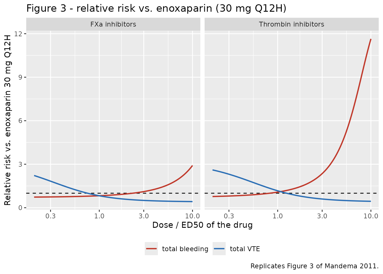

# Invert each relative-risk curve for the dose multiple at which RR crosses 1.
window <- function(label) {
  d <- fig3 |> dplyr::filter(class == label)
  eff <- d |> dplyr::filter(endpoint == "total VTE")
  bld <- d |> dplyr::filter(endpoint == "total bleeding")
  r_lo <- stats::approx(x = eff$rr, y = eff$r, xout = 1)$y  # efficacy parity
  r_hi <- stats::approx(x = bld$rr, y = bld$r, xout = 1)$y  # bleeding parity
  cross_rr <- stats::approx(
    x = eff$rr - bld$rr, y = eff$rr,
    xout = 0)$y
  c(r_lo = r_lo, r_hi = r_hi, width = r_hi / r_lo, cross_rr = cross_rr)
}

w_fxa <- window("FXa inhibitors")
w_thr <- window("Thrombin inhibitors")

# FXa: a benefit window exists and is about threefold wide.
stopifnot(w_fxa[["width"]] > 2.5, w_fxa[["width"]] < 3.5)
# FXa: the two curves cross at about a 17% reduction in relative risk.
stopifnot(abs((1 - w_fxa[["cross_rr"]]) - 0.17) < 0.02)
# Thrombin inhibitors: the window is inverted, i.e. no dose gives both benefits.
stopifnot(w_thr[["r_hi"]] < w_thr[["r_lo"]])

cat(sprintf("FXa inhibitors: benefit window %.2f-%.2f x ED50 (%.2f-fold wide); curves cross at a %.1f%% reduction\n",
            w_fxa[["r_lo"]], w_fxa[["r_hi"]], w_fxa[["width"]], 100 * (1 - w_fxa[["cross_rr"]])))
#> FXa inhibitors: benefit window 0.75-2.28 x ED50 (3.04-fold wide); curves cross at a 17.4% reduction
cat(sprintf("Thrombin inhibitors: efficacy parity at %.2f x ED50 but bleeding parity already at %.2f x ED50 -- no window\n",
            w_thr[["r_lo"]], w_thr[["r_hi"]]))
#> Thrombin inhibitors: efficacy parity at 1.25 x ED50 but bleeding parity already at 0.82 x ED50 -- no window

Absolute event rates for enoxaparin

The source reports observed absolute total-VTE incidence under enoxaparin of 13.5% after hip replacement and 28.6% after knee replacement, pooled across doses, with a between-trial range of 1.7% to 46%. Those absolute levels are driven by the per-trial intercepts rather than by the dose-response, so the model - whose intercepts describe the single reference trial drawn in Figure 1 - should land in the lower part of that range, near the hip-surgery value.

enox_regimens <- tibble::tibble(
  regimen = c("20 mg b.i.d. (Japan)", "40 mg q.d. (Europe)", "30 mg Q12H (North America)"),
  dose    = c(40, 40, 60)
)

enox_pred <- rxode2::rxSolve(
  mod,
  events = as.data.frame(make_arms("enoxaparin", enox_regimens$dose)),
  returnType = "data.frame"
)

enox_regimens |>
  dplyr::mutate(
    `Total VTE (%)`      = round(100 * enox_pred$p_totalvte, 1),
    `Major VTE (%)`      = round(100 * enox_pred$p_majorvte, 1),
    `PE (%)`             = round(100 * enox_pred$p_pe, 2),
    `Major bleeding (%)` = round(100 * enox_pred$p_majorbld, 2),
    `Total bleeding (%)` = round(100 * enox_pred$p_totalbld, 1)
  ) |>
  dplyr::rename("Enoxaparin regimen" = regimen, "Daily dose (mg)" = dose) |>
  knitr::kable(caption = "Predicted per-arm incidence for the three approved enoxaparin regimens.")

Predicted per-arm incidence for the three approved enoxaparin regimens.
Enoxaparin regimen	Daily dose (mg)	Total VTE (%)	Major VTE (%)	PE (%)	Major bleeding (%)	Total bleeding (%)
20 mg b.i.d. (Japan)	40	14.5	4.3	0.27	1.00	6.2
40 mg q.d. (Europe)	40	14.5	4.3	0.27	1.00	6.2
30 mg Q12H (North America)	60	10.9	2.9	0.18	1.21	7.0


# Predicted total VTE under enoxaparin must sit inside the reported 1.7-46%
# between-trial range and within a few points of the 13.5% hip-surgery figure.
stopifnot(all(enox_pred$p_totalvte > 0.017), all(enox_pred$p_totalvte < 0.46))
stopifnot(abs(100 * enox_pred$p_totalvte[2] - 13.5) < 3)

Warfarin has no bleeding dose-response

The source could not estimate EDbld for warfarin (“The TI for warfarin could not be estimated”), and Table 2 omits warfarin entirely. The model reports this explicitly rather than silently predicting a placebo bleeding rate for warfarin arms.

warf <- sim |> dplyr::filter(drug == "warfarin")

stopifnot(all(warf$warfarin_bleeding_undefined == 1))
# Bleeding predictions for warfarin equal the control-arm rate: no dose-response.
stopifnot(max(abs(warf$p_majorbld - ilogit(e0[["majorbld"]]))) < 1e-12)
# The efficacy side IS estimated for warfarin, so it must move with dose.
stopifnot(diff(range(warf$p_totalvte)) > 0)

cat("warfarin arms flagged as bleeding-undefined:", sum(warf$warfarin_bleeding_undefined),
    "of", nrow(warf), "\n")
#> warfarin arms flagged as bleeding-undefined: 60 of 60

No PKNCA validation

PKNCA is deliberately not used here. There is no concentration-time profile to integrate: the model has no PK layer, no ODE states and no time axis, and its outputs are per-arm event probabilities. The validation above instead follows the pattern for mechanistic / non-PK models - reproduce the source’s own published quantitative claims:

the placebo intercepts (exact),
the potency collapse of all 23 drugs onto one major-VTE curve (exact),
the bleeding slope ratios between endpoints (exact),
all 30 off-diagonal cells of the published Table 2,
both total-VTE relative TI values quoted in the Results,
the Figure 3 threefold benefit window and 17% crossing,
the absence of a warfarin bleeding dose-response.

Assumptions and deviations

Non-paper-derived parameter values - the six e0_* intercepts. Mandema 2011 estimated a separate placebo-response intercept for each of the 89 trials and reports none of them, so no published table can supply an absolute event rate. The six values in ini() were recovered by digitizing the published enoxaparin dose-response curves in Figures 1 and 2: the page was rendered at 200 dpi, the axes were calibrated from the printed tick marks, the solid (fitted) curve was traced column by column, and E0 was solved at every extracted point using the source’s own published Emax, ED50, n, EDbld and Sc values. The recovered E0 was essentially constant along each curve (interquartile range 0.009 to 0.023 on the logit scale, under +/- 0.15 percentage points of incidence), which is itself strong evidence that the equations and parameter values encoded in the model file reproduce the published figures. Treat these six values as describing the single reference trial drawn in the figures, not any particular study; real trials ranged from 1.7% to 46% total VTE. Every other value in the model comes from the supplement’s parameter table.
Sign convention for the bleeding term. The Methods write the general structure with a single minus sign, P(event) = f{E0 - g(...)}. That sign is correct for the efficacy endpoints, where the dose-response is a risk reduction. For bleeding the term must be added: Figure 2 shows bleeding incidence rising with dose, Figure 3 shows bleeding relative risk crossing 1 from below, and the Discussion describes “the steep inflection point for increased bleeding risk if the dose increases above the equivalent of 100 mg/day enoxaparin”. The model therefore uses E0 - g for efficacy and E0 + g for bleeding.
Placement of the (1 + Sc) bleeding-endpoint factor. The supplement’s two dose-response equations are embedded as Equation Editor objects rather than as text, so they do not survive into the extracted document. They were recovered from the embedded objects and cross-checked three ways: the efficacy equation matches the sigmoid Emax form printed in the main text verbatim; the glossary beneath the equations describes Sc as “the fractional change in the slope of the bleeding dose response relationship”, which requires the factor to multiply the slope rather than the EDbld denominator; and the main text states that “the slope of the dose-response relationship for total bleeding was smaller than that for major bleeding”, which only the multiplying form reproduces with a negative Sc. Fitting both candidate forms to the digitized Figure 2 curves settles it decisively - the encoded form recovers a constant intercept (interquartile range 0.013 to 0.015 on the logit scale) while the alternative reading does not (0.51 to 0.85, i.e. 40 to 60 times worse).
Reference levels are encoded as literal constants, not parameters. The enoxaparin total-VTE class ratio is 1 and the major-bleeding Sc is 0 by definition of the reference category; the supplement tabulates only the non-reference levels, so no ini() entry is created for them.
No random effects and no residual error. Trial-level random effects on Emax and ED50 were tested by the source and rejected (“the estimated variances were close to zero”), and the observations were event counts under a binomial likelihood rather than continuous measurements, so there is no residual SD to encode. Simulations from this model are deterministic. A user who wants simulated counts should draw rbinom(n = n_arm, size = 1, prob = p_<endpoint>) downstream, which is what the source’s likelihood assumes. The within-arm compound-symmetry correlation across endpoints is a property of the estimation, not of the predictive model, and is not encoded.
Simulation scope. Predictions are per-arm (study-arm-mean) event probabilities. This model cannot produce individual-subject events, and it has no PK layer, so it cannot be linked to exposure without an external dose-to-exposure model.
One drug per arm. Every trial arm in the source received exactly one anticoagulant, so the model sums potency-normalised doses across the CONMED_<drug>_DOSE columns knowing that at most one is non-zero. Coding two drugs simultaneously is outside the source’s calibration range and would make the model add their normalised doses.
Warfarin dose units. CONMED_WARFARIN_DOSE carries an achieved INR, not a milligram dose, because warfarin is titrated to an INR target and the source models it that way (Table 1 gives its “daily dose range” as 2.2-2.5 INR and the supplement gives ED50 Warfarin (INR) = 4.05). Warfarin also has no EDbld, so its bleeding predictions collapse to the control-arm rate; the model flags this through warfarin_bleeding_undefined.
Certoparin. It appears in the Methods literature-search term list but no certoparin trial met the inclusion criteria, so it has no ED50 in the supplement and no dose column in this model.
Desirudin and SR123781A. Both are the sole members of their classes and both were excluded from the source’s Table 2 pairwise comparison “because only limited data are available for each”. Their parameters are encoded (the bivalent-thrombin EDbld ratio has a 95% CI of 0.652 to 21.3), but they are omitted from the Table 2 replication above for the same reason the source omitted them.
Dose-grid choice in the virtual cohort. Two drugs (bemiparin and dalteparin) were each studied at a single daily dose, so a log-spaced grid over their reported range would be degenerate. The cohort code widens any such range to a factor of 20 below the upper dose purely so the figures show a curve rather than a point; this affects the plotted range only, not any gate.