Gemcabene, statins and ezetimibe LDL-C MBMA (Mandema 2005)

Model and source

• Citation: Mandema JW, Hermann D, Wang W, Sheiner T, Milad M, Bakker-Arkema R, Hartman D. Model-based development of gemcabene, a new lipid-altering agent. AAPS J. 2005 Oct 7;7(3):E513-E522. doi:10.1208/aapsj070352. Model structure is Equations 1 and 2 (Materials and Methods, Statistical Analysis); all parameter estimates are in Table 2.
• Description: MBMA. Model-based meta-analysis dose-response model for the percentage change in low-density lipoprotein cholesterol (LDL-C) from pretreatment baseline for five statins (atorvastatin, rosuvastatin, simvastatin, lovastatin, pravastatin), the cholesterol absorption inhibitor ezetimibe, the investigational lipid-altering agent gemcabene, and statin-plus-nonstatin combinations. Fit to study-arm summary means from 25 randomized controlled trials (9,886 patients) by nonlinear mixed-effects regression in S-PLUS 6.1. Each drug follows a sigmoid Emax dose-response in daily dose; the five statins share a common Emax (-78.7 percent) and a common shallow Hill coefficient (0.451) and differ only in ED50 (potency), while ezetimibe and gemcabene each carry their own Emax, ED50 and Hill coefficient. Combination therapy uses the multiplicative interaction term 0.01 * g * Estatin * Enonstatin, where g = 1 is pharmacological independence: ezetimibe was found independent (g fixed to 1, giving added LDL-C lowering across the whole statin dose range) whereas gemcabene was significantly LESS than independent (g = 1.69), so gemcabene adds almost nothing on top of a high statin dose. Per-arm daily dose enters through one CONMED__DOSE column per drug (0 outside that drug’s arm; all zero = placebo) and European trials carry an extra 4 percent LDL-C reduction on the placebo intercept. The trial-specific random-effect variance was not significantly different from zero and the between-subject residual variance is not reported numerically, so the model has no eta and its residual SD is fixed to zero. Suitable simulation scope is the study-arm mean percentage change in LDL-C, NOT individual-subject responses; there is no PK layer and no time course.
• Article: https://doi.org/10.1208/aapsj070352 (PMC2751254, open access)

This is a model-based meta-analysis (MBMA) built to support a go/no-go decision on gemcabene, an investigational lipid-altering agent (development code CI-1027). The analysis pooled published statin and ezetimibe trials with four Pfizer-sponsored gemcabene trials so that gemcabene could be compared against its competitors on a common dose-response scale, including in combination with a statin. On the strength of this model the sponsor stopped development: the model showed that gemcabene’s benefit on top of a statin collapses at high statin doses, unlike ezetimibe’s.

Population

Mandema 2005 fitted study-arm summary means from 25 randomized controlled trials totalling 9,886 patients (the paper’s Abstract rounds this to “almost 10,000”). Twenty-one trials evaluated statins, ezetimibe, or their combination in patients with hypercholesterolemia; all were randomized, double-blind, multiple-dose once-daily parallel-group studies, 13 of them placebo controlled, and most multicentre. They were identified by a Medline search with a 31 May 2003 cut-off (minimum 4 weeks of treatment), supplemented by FDA summary-basis-of-approval documents.

Four further trials came from the gemcabene programme. Three studied gemcabene monotherapy in healthy volunteers, nondiabetic healthy obese subjects, and subjects with low HDL-C and normal or elevated triglycerides; the fourth was the phase IIA hypercholesterolemia trial that crossed gemcabene 300/600/900 mg/day with atorvastatin 10/20/80 mg/day. Three of the four were unpublished at the time of writing.

Daily doses spanned atorvastatin 2.5-80 mg, rosuvastatin 1-80 mg, simvastatin 10-80 mg, lovastatin 10-80 mg, pravastatin 10-40 mg, ezetimibe 0.25-40 mg, and gemcabene 50-900 mg (Table 1). Baseline LDL-C ranged 112-217 mg/dL across trials. Critically, the three gemcabene healthy-subject trials had much lower baseline LDL-C (112-120 mg/dL) than the hypercholesterolemia trials (165-217 mg/dL). The paper handled that mismatch upstream rather than in the dose-response model: a per-trial ANOVA over those three trials (factors dose, trial, baseline LDL-C, triglycerides) found “a small impact of baseline LDL-C values < 100 mg/dL” and no treatment-by-baseline interaction, and its least-squares means were then used as the summary data fed to the dose-response analysis.

Each modelled observation is therefore a study-arm mean percentage change in LDL-C from pretreatment baseline, not an individual patient value. The simulation scope of this model is the study-arm mean; it is not suitable for individual-subject simulation, and it has no PK layer and no time course.

The same information is available programmatically via rxode2::rxode(readModelDb("Mandema_2005_gemcabene_mbma"))$population.

Source trace

The model is Equations 1 and 2 of the paper (Materials and Methods, Statistical Analysis). Equation 1 combines a statin with a nonstatin:

$$Y = E_0 + E_{\text{statin}} + E_{\text{nonstatin}} + 0.01 \cdot g \cdot E_{\text{statin}} \cdot E_{\text{nonstatin}} + \eta + \varepsilon$$

and Equation 2 is a sigmoid Emax dose-response applied to each drug:

$$E_{\text{drug}} = \frac{\text{Dose}^{n} \cdot E_{\max}}{\text{Dose}^{n} + \text{ED}_{50}^{n}}$$

$Y$ is the percentage change in LDL-C from pretreatment baseline, so every $E$ term is on the percent scale and a negative value is a reduction. The factor $0.01$ is exactly what converts a product of two percentages back into a percentage: at $g = 1$ Equation 1 reproduces pharmacological independence, $1 - (1 - f_{\text{statin}})(1 - f_{\text{nonstatin}})$ on the fractional scale. $g > 1$ means less than independent.

Equation / parameter	Value	Source location
Combination structure (Eq 1)	n/a	Methods, Statistical Analysis, p. E514
Sigmoid Emax dose-response (Eq 2)	n/a	Methods, Statistical Analysis, p. E514
e0 (placebo effect, North American trials)	0.802 %	Table 2, E0 [0.0598 to 1.54]
e_region_europe_e0 (extra European placebo reduction)	-4 %	Results, LDL-C section (prose only; no Table 2 row, no CI)
emax_statin (shared across all five statins)	-78.7 %	Table 2, Emax, statin (%) [-90.7 to -66.7]
led50_atorvastatin	13.1 mg/day	Table 2, ED50, Atorvastatin (mg) [6.57 to 26.2]
led50_rsv	4.35 mg/day	Table 2, ED50, Rosuvastatin (mg) [2.19 to 8.62]
led50_smv	30.5 mg/day	Table 2, ED50, Simvastatin (mg) [15 to 62.1]
led50_lov	82.8 mg/day	Table 2, ED50, Lovastatin (mg) [37.1 to 185]
led50_prv	97.3 mg/day	Table 2, ED50, Pravastatin (mg) [42.4 to 223]
ln_statin (Hill coefficient, shared across statins)	0.451	Table 2, n statin [0.366 to 0.557]
emax_ezt	-19.6 %	Table 2, Emax,Ezetimibe (%) [-20.6 to -18.6]
led50_ezt	0.302 mg/day	Table 2, ED50,Ezetimibe (mg) [0.151 to 0.604]
ln_ezt (ezetimibe Hill coefficient; held constant)	1	Table 2, n Ezetimibe (no CI); Results: “A Hill coefficient for ezetimibe could not be estimated and was fixed to 1.”
gamma_ezt (statin x ezetimibe interaction; held constant)	1	Table 2, g Ezetimibe (no CI); Results: “not statistically significantly different from 1 and was, therefore, fixed to this pharmacological value”
emax_gem	-34.8 %	Table 2, Emax,gemcabene (%) [-45 to -24.6]
led50_gem	314 mg/day	Table 2, ED50,gemcabene (mg) [220 to 448]
ln_gem (gemcabene Hill coefficient)	2.27	Table 2, n gemcabene [1.19 to 4.34]
gamma_gem (statin x gemcabene interaction)	1.69	Table 2, g gemcabene [1.49 to 1.88]; Results also give 1.69 +/- 0.10 (mean +/- SE), p < 0.001 versus 1
Trial random-effect variance (nu^2, Eq 1)	not encoded	Results: “The variance of the trial-specific random effect was found to be not statistically significantly different from zero”; no numeric estimate published
Residual variance (sigma^2, Eq 1)	addSd held at 0	Eq 1 declares eps ~ N(0, sigma^2); no numeric value for sigma is published anywhere in the paper

A note on the published PDF’s minus signs

The AAPS Journal PDF renders the minus sign of every negative Table 2 entry as a leading digit 2 (so Emax, statin prints as 278.7 for -78.7, and Emax,gemcabene as 234.8 for -34.8). The same substitution turns g = 1.69 +/- 0.10 into g 5 1.69 6 0.10. The signs used in the model file are not a guess: they are confirmed end-to-end by reproducing every cell of the paper’s own Table 3 from Table 2, which is done below.

Errata

No published erratum, corrigendum, or author correction was located for Mandema 2005. Searches of the AAPS Journal / PMC landing page for PMC2751254, the DOI 10.1208/aapsj070352, and PubMed (PMID 16353928) returned no correction notices as of the extraction date (2026-09-01).

Reporting gaps in the paper as published (not errata, but they constrain what can be encoded):

• No numeric estimate of the residual SD sigma is given anywhere, although Equation 1 declares it.
• The 4% larger placebo response in European trials appears only as a prose sentence, to one significant figure, with no Table 2 row and no confidence interval.
• Table 2 reports marginal 95% confidence intervals but not the variance-covariance matrix, so the paper’s own uncertainty bands (derived from 5,000 parameter draws) cannot be reproduced. See Assumptions below.

Virtual cohort

There is no cohort to simulate in the usual sense: the model is a deterministic, time-independent, per-arm dose-response with no between-subject variability, no trial random effect (its variance was not different from zero), and a residual SD held at zero. Every check below is therefore a deterministic comparison against a published number, and the assertions are correspondingly tight – there is no simulated cohort whose extreme could shift between rxode2 versions or thread counts.

Each “subject” in the event tables below is one study arm: a set of per-drug daily doses plus the trial’s region indicator.

mod <- readModelDb("Mandema_2005_gemcabene_mbma")

# Every covariate column the model consumes, defaulted to a North American
# placebo arm. Helper `arm()` overrides only what a given arm actually gets.
arm_template <- list(
  CONMED_ATORVASTATIN_DOSE = 0,
  CONMED_RSV_DOSE          = 0,
  CONMED_SMV_DOSE          = 0,
  CONMED_LOV_DOSE          = 0,
  CONMED_PRV_DOSE          = 0,
  CONMED_EZT_DOSE          = 0,
  CONMED_GEMCABENE_DOSE    = 0,
  REGION_EUROPE            = 0
)

arm <- function(...) {
  over <- list(...)
  stopifnot(all(names(over) %in% names(arm_template)))
  as.data.frame(utils::modifyList(arm_template, over))
}

# Solve a data.frame of arms and return it with the predicted percentage
# change in LDL-C attached. The model is algebraic, so each arm is a single
# time-0 observation record; `keep` carries the labelling columns through.
solve_arms <- function(arms, keep = character()) {
  ev <- arms
  ev$id   <- seq_len(nrow(ev))
  ev$time <- 0
  ev$amt  <- 0
  ev$evid <- 0L
  # `mod` is eta-free, so `omega = NA` is unnecessary and errors on the
  # released rxode2 (5.1.6: "invalid 'times' argument").
  out <- as.data.frame(rxode2::rxSolve(mod, events = ev))
  stopifnot(nrow(out) == nrow(arms), !anyNA(out$Cc))
  cbind(arms[keep], pct_change_ldlc = out$Cc)
}

Replication: statin monotherapy dose-response (Figure 1)

Figure 1 of the paper plots the model-predicted mean percentage LDL-C reduction against dose for each of the five statins. The defining structural finding is that the statins share one Emax and one (shallow) Hill coefficient and differ only in ED50: “none of the statins had a statistically significant effect on Emax when tested independently … a similar maximal effect of about 79% reduction in LDL-C over placebo.”

statin_cols <- c(
  Atorvastatin = "CONMED_ATORVASTATIN_DOSE",
  Rosuvastatin = "CONMED_RSV_DOSE",
  Simvastatin  = "CONMED_SMV_DOSE",
  Lovastatin   = "CONMED_LOV_DOSE",
  Pravastatin  = "CONMED_PRV_DOSE"
)

dose_grid <- c(0.5, 1, 2.5, 5, 10, 20, 40, 80, 160)

statin_arms <- dplyr::bind_rows(lapply(names(statin_cols), function(sn) {
  a <- dplyr::bind_rows(lapply(dose_grid, function(d) {
    x <- list(d); names(x) <- statin_cols[[sn]]
    do.call(arm, x)
  }))
  a$statin <- sn
  a$dose   <- dose_grid
  a
}))

statin_curves <- solve_arms(statin_arms, keep = c("statin", "dose"))
#> Warning: multi-subject simulation without without 'omega'

ggplot(statin_curves, aes(x = dose, y = pct_change_ldlc, colour = statin)) +
  geom_line(linewidth = 0.9) +
  geom_point(size = 1.3) +
  scale_x_log10(breaks = c(0.5, 1, 2.5, 5, 10, 20, 40, 80, 160)) +
  labs(
    x      = "Daily statin dose (mg/day, log scale)",
    y      = "LDL-C % change from pretreatment",
    colour = NULL,
    title  = "Mandema 2005 Figure 1 -- statin monotherapy dose-response",
    caption = "Shared Emax (-78.7%) and Hill coefficient (0.451); statins differ only in ED50."
  ) +
  theme_bw() +
  theme(legend.position = "top")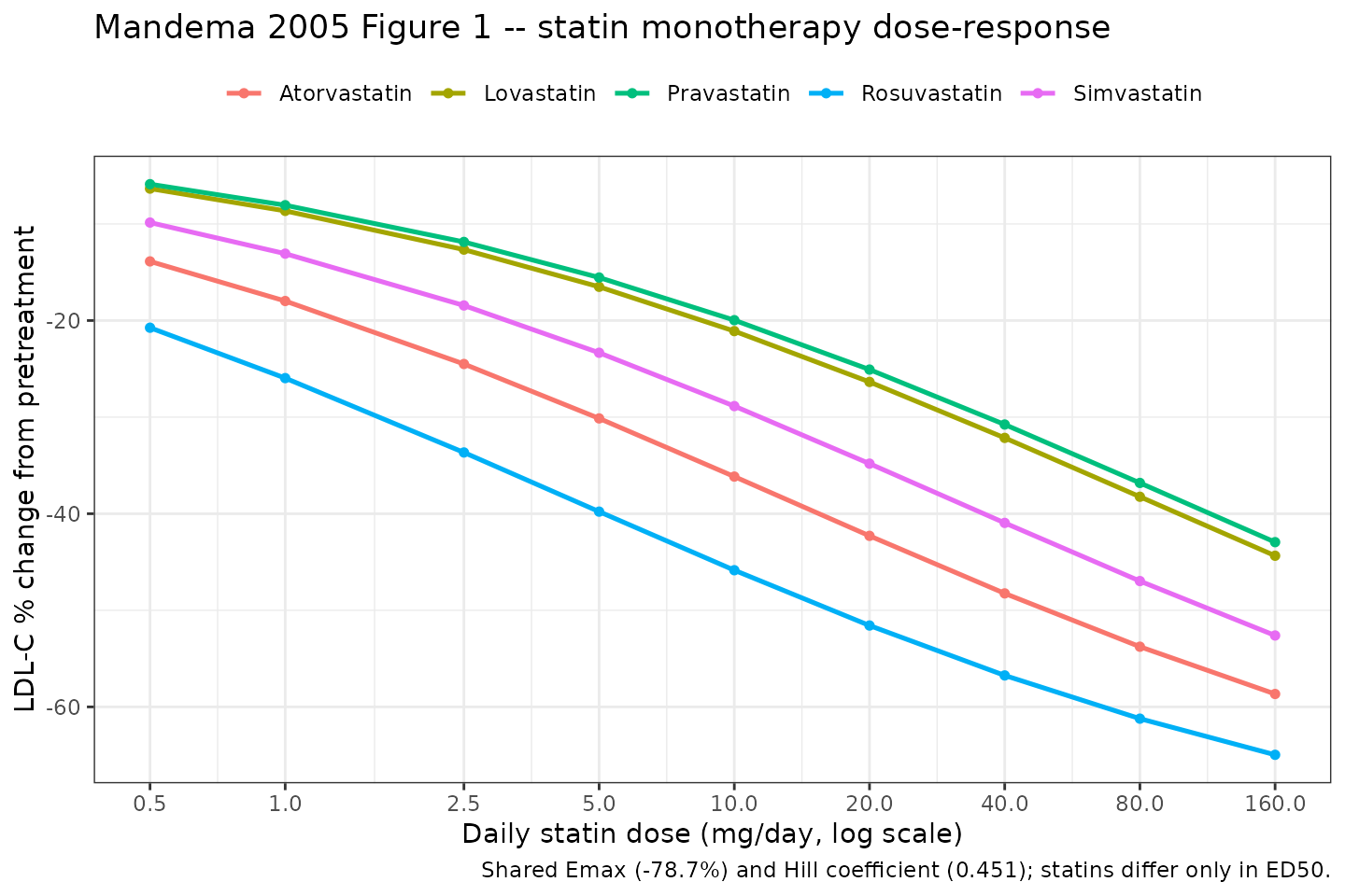

Replicates Figure 1 of Mandema 2005: model-predicted percentage change in LDL-C for monotherapy with each of the five statins. The five curves are the same shape shifted along the log-dose axis; only ED50 differs.

Shared-Emax and relative-potency checks

The Discussion states the relative potencies of rosuvastatin, simvastatin, lovastatin and pravastatin against atorvastatin as 0.33, 2.3, 6.3 and 7.4, and gives the doses equivalent to 10 mg atorvastatin as 3.3, 23, 63 and 74 mg. Both are pure ED50 ratios under the shared-Emax structure, so they test whether the five ED50 values were transcribed correctly and whether the shared-Emax structure was implemented as the authors described it.

ed50 <- c(Atorvastatin = 13.1, Rosuvastatin = 4.35, Simvastatin = 30.5,
          Lovastatin = 82.8, Pravastatin = 97.3)
others <- c("Rosuvastatin", "Simvastatin", "Lovastatin", "Pravastatin")

potency <- data.frame(
  Statin            = others,
  potency_model     = round(unname(ed50[others] / ed50[["Atorvastatin"]]), 2),
  potency_paper     = c(0.33, 2.3, 6.3, 7.4),
  equiv_dose_model  = round(10 * unname(ed50[others] / ed50[["Atorvastatin"]]), 1),
  equiv_dose_paper  = c(3.3, 23, 63, 74)
)

knitr::kable(
  potency |>
    dplyr::rename(
      "Relative potency (model)"      = potency_model,
      "Relative potency (paper)"      = potency_paper,
      "Dose equal to atorvastatin 10 mg, model (mg)" = equiv_dose_model,
      "Dose equal to atorvastatin 10 mg, paper (mg)" = equiv_dose_paper
    ),
  caption = "Relative statin potencies against atorvastatin (Mandema 2005 Discussion). Deterministic ED50 ratios."
)

Relative statin potencies against atorvastatin (Mandema 2005 Discussion). Deterministic ED50 ratios.

Statin	Relative potency (model)	Relative potency (paper)	Dose equal to atorvastatin 10 mg, model (mg)	Dose equal to atorvastatin 10 mg, paper (mg)
Rosuvastatin	0.33	0.33	3.3	3.3
Simvastatin	2.33	2.30	23.3	23.0
Lovastatin	6.32	6.30	63.2	63.0
Pravastatin	7.43	7.40	74.3	74.0

# Both sides are the same published ED50 values; the only difference is the
# paper's rounding to two significant figures, so these bounds are tight.
stopifnot(
  max(abs(potency$potency_model - potency$potency_paper)) < 0.05,
  max(abs(potency$equiv_dose_model - potency$equiv_dose_paper) /
        potency$equiv_dose_paper) < 0.02
)

# Emax check: at an effectively infinite statin dose the model must return the
# shared Emax of -78.7% (paper Results: "about 79% reduction ... over placebo").
# The probe dose has to be absurdly large precisely because the statin Hill
# coefficient is 0.451: the approach to Emax goes as (ED50/Dose)^0.451, so
# 1e9 mg is still 0.02 percentage points short while 1e15 mg is within 1e-3.
# That slow approach IS the paper's "shallow dose-response relationship ...
# the maximum efficacy is more difficult to achieve" (Discussion).
emax_chk <- solve_arms(arm(CONMED_ATORVASTATIN_DOSE = 1e15))$pct_change_ldlc -
  solve_arms(arm())$pct_change_ldlc
cat(sprintf("Statin effect at infinite dose: %.2f%% (Table 2 Emax,statin = -78.7%%)\n",
            emax_chk))
#> Statin effect at infinite dose: -78.70% (Table 2 Emax,statin = -78.7%)
stopifnot(abs(emax_chk - (-78.7)) < 0.01)

Replication: ezetimibe and gemcabene monotherapy (Figures 2 and 4)

Figure 2 shows ezetimibe monotherapy and Figure 4 shows gemcabene monotherapy. The two nonstatins behave very differently: ezetimibe has a low Emax (-19.6%) but an ED50 of only about 0.3 mg, so the marketed 10 mg dose sits essentially at its maximum; gemcabene has a larger Emax (-34.8%) but an ED50 of 314 mg and a steep Hill coefficient of 2.27, so 900 mg is still short of its maximum.

ezt_grid <- c(0.05, 0.1, 0.25, 0.5, 1, 2.5, 5, 10, 20, 40)
gem_grid <- c(25, 50, 100, 150, 300, 450, 600, 900, 1800)

nonstatin_curves <- dplyr::bind_rows(
  solve_arms(
    dplyr::bind_rows(lapply(ezt_grid, function(d) arm(CONMED_EZT_DOSE = d))) |>
      dplyr::mutate(drug = "Ezetimibe", dose = ezt_grid),
    keep = c("drug", "dose")
  ),
  solve_arms(
    dplyr::bind_rows(lapply(gem_grid, function(d) arm(CONMED_GEMCABENE_DOSE = d))) |>
      dplyr::mutate(drug = "Gemcabene", dose = gem_grid),
    keep = c("drug", "dose")
  )
)
#> Warning: multi-subject simulation without without 'omega'
#> Warning: multi-subject simulation without without 'omega'

studied <- dplyr::bind_rows(
  data.frame(drug = "Ezetimibe", dose = c(0.25, 1, 5, 10, 20, 40)),
  data.frame(drug = "Gemcabene", dose = c(50, 150, 300, 450, 600, 900))
) |>
  dplyr::inner_join(nonstatin_curves, by = c("drug", "dose"))

ggplot(nonstatin_curves, aes(x = dose, y = pct_change_ldlc)) +
  geom_line(linewidth = 0.9, colour = "steelblue") +
  geom_point(data = studied, size = 2, colour = "black") +
  facet_wrap(~ drug, scales = "free_x") +
  scale_x_log10() +
  labs(
    x = "Daily dose (mg/day, log scale)",
    y = "LDL-C % change from pretreatment",
    title = "Mandema 2005 Figures 2 and 4 -- nonstatin monotherapy dose-response",
    caption = "Black points mark the dose strengths actually studied (Table 1)."
  ) +
  theme_bw()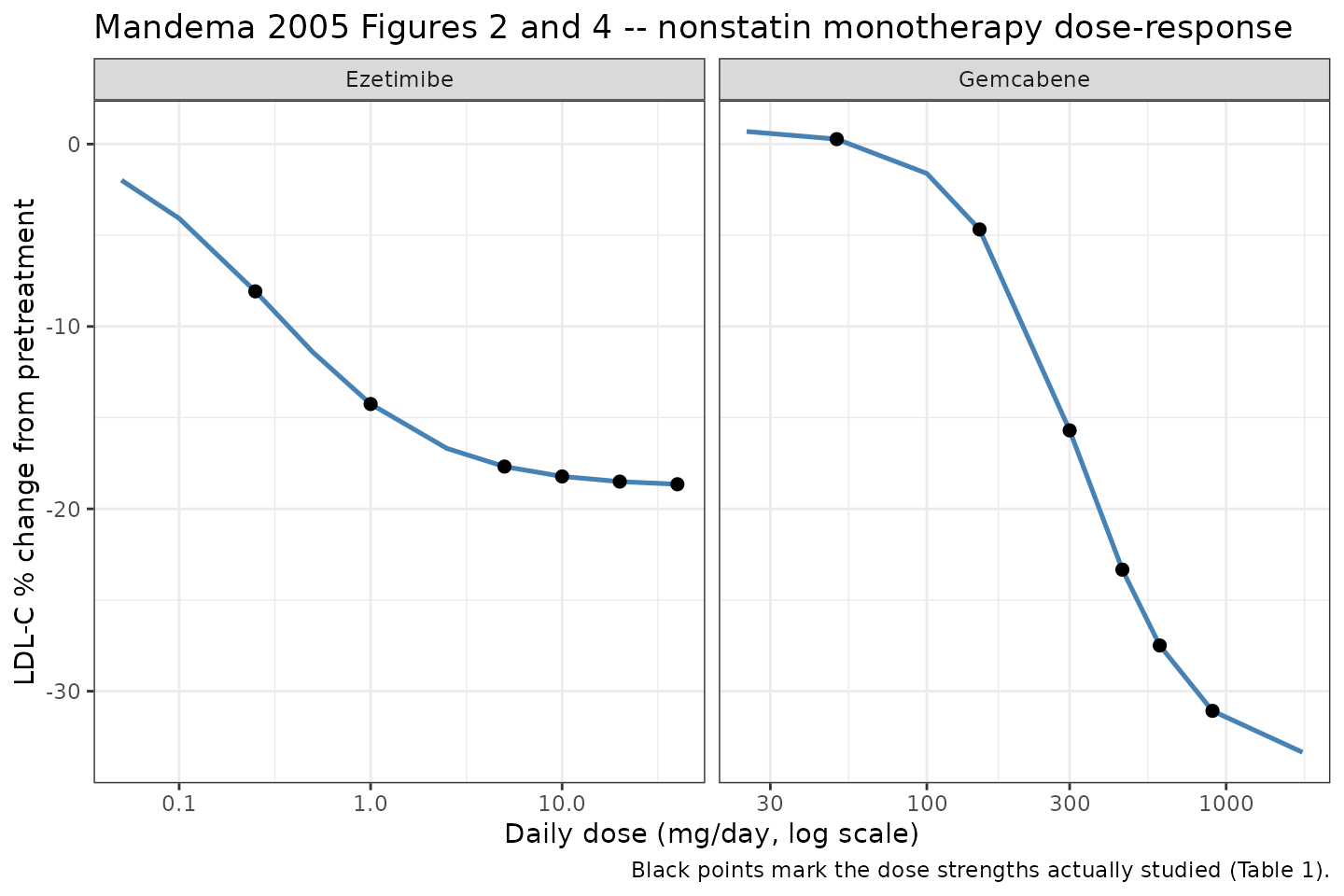

Replicates Figures 2 and 4 of Mandema 2005: monotherapy dose-response for ezetimibe (ED50 0.302 mg, Hill 1) and gemcabene (ED50 314 mg, Hill 2.27). Points mark the doses each drug was actually studied at (Table 1).

The Discussion gives two point predictions for monotherapy, which are the strictest available single-drug checks:

placebo <- solve_arms(arm())$pct_change_ldlc

mono <- data.frame(
  Treatment = c("Gemcabene 900 mg", "Ezetimibe 10 mg"),
  model = c(
    solve_arms(arm(CONMED_GEMCABENE_DOSE = 900))$pct_change_ldlc - placebo,
    solve_arms(arm(CONMED_EZT_DOSE = 10))$pct_change_ldlc - placebo
  ),
  paper = c(-31.9, -19.1)
)
mono$model <- round(mono$model, 2)

knitr::kable(
  mono |>
    dplyr::rename("Model (% change)" = model, "Paper (% change)" = paper),
  caption = "Monotherapy predictions quoted in the Mandema 2005 Discussion. Deterministic; differences are the paper's rounding of Table 2 inputs to three significant figures."
)

Monotherapy predictions quoted in the Mandema 2005 Discussion. Deterministic; differences are the paper’s rounding of Table 2 inputs to three significant figures.

Treatment	Model (% change)	Paper (% change)
Gemcabene 900 mg	-31.88	-31.9
Ezetimibe 10 mg	-19.03	-19.1

stopifnot(max(abs(mono$model - mono$paper)) < 0.15)

Replication: the interaction between statins and the two nonstatins (Figures 3, 5, 6 and Table 3)

This is the heart of the paper, and the reason gemcabene was stopped. Table 3 tabulates the additional mean LDL-C change from adding 900 mg gemcabene or 10 mg ezetimibe on top of atorvastatin monotherapy at 0, 10, 20, 40 and 80 mg. Because Table 3 reports within-trial differences, the intercept e0 (and any trial-level region effect) cancels exactly.

Table 3 is an independent output: it is not an input to the model, and every cell in it is a nonlinear function of all of Table 2. Reproducing all ten mean cells is therefore a genuine end-to-end confirmation of the structural form, the parameter transcription, and every sign.

ator_doses <- c(0, 10, 20, 40, 80)

mono_ator <- solve_arms(
  dplyr::bind_rows(lapply(ator_doses, function(d) arm(CONMED_ATORVASTATIN_DOSE = d)))
)$pct_change_ldlc
#> Warning: multi-subject simulation without without 'omega'

add_gem <- solve_arms(
  dplyr::bind_rows(lapply(ator_doses, function(d) {
    arm(CONMED_ATORVASTATIN_DOSE = d, CONMED_GEMCABENE_DOSE = 900)
  }))
)$pct_change_ldlc
#> Warning: multi-subject simulation without without 'omega'

add_ezt <- solve_arms(
  dplyr::bind_rows(lapply(ator_doses, function(d) {
    arm(CONMED_ATORVASTATIN_DOSE = d, CONMED_EZT_DOSE = 10)
  }))
)$pct_change_ldlc
#> Warning: multi-subject simulation without without 'omega'

table3 <- data.frame(
  atorvastatin_mg = ator_doses,
  gem_model = round(add_gem - mono_ator, 1),
  gem_paper = c(-31.9, -12.0, -8.7, -5.5, -2.5),
  ezt_model = round(add_ezt - mono_ator, 1),
  ezt_paper = c(-19.1, -12.0, -10.8, -9.7, -8.7)
)

knitr::kable(
  table3 |>
    dplyr::rename(
      "Atorvastatin (mg)"         = atorvastatin_mg,
      "+900 mg gemcabene (model)" = gem_model,
      "+900 mg gemcabene (paper)" = gem_paper,
      "+10 mg ezetimibe (model)"  = ezt_model,
      "+10 mg ezetimibe (paper)"  = ezt_paper
    ),
  caption = "Replicates Mandema 2005 Table 3: additional mean % change in LDL-C from adding 900 mg gemcabene or 10 mg ezetimibe to atorvastatin monotherapy. Paper columns are the 'Mean' entries of Table 3."
)

Replicates Mandema 2005 Table 3: additional mean % change in LDL-C from adding 900 mg gemcabene or 10 mg ezetimibe to atorvastatin monotherapy. Paper columns are the ‘Mean’ entries of Table 3.

Atorvastatin (mg)	+900 mg gemcabene (model)	+900 mg gemcabene (paper)	+10 mg ezetimibe (model)	+10 mg ezetimibe (paper)
0	-31.9	-31.9	-19.0	-19.1
10	-12.0	-12.0	-12.0	-12.0
20	-8.7	-8.7	-10.8	-10.8
40	-5.5	-5.5	-9.7	-9.7
80	-2.5	-2.5	-8.6	-8.7

t3_err <- c(abs(table3$gem_model - table3$gem_paper),
            abs(table3$ezt_model - table3$ezt_paper))
cat(sprintf("Max absolute deviation across all 10 Table 3 mean cells: %.2f percentage points\n",
            max(t3_err)))
#> Max absolute deviation across all 10 Table 3 mean cells: 0.10 percentage points

# Deterministic: both sides are the published Table 2 parameters evaluated
# through the published Equations 1-2. The only source of difference is that
# the paper rounded Table 2 to three significant figures before computing
# Table 3 and then rounded Table 3 to one decimal place. A transposed digit,
# a dropped minus sign, or a wrong interaction coefficient moves these cells
# by whole percentage points, so 0.15 still fails loudly.
stopifnot(max(t3_err) <= 0.15)

fig6_grid <- c(0, 1, 2.5, 5, 10, 20, 40, 80)

fig6 <- dplyr::bind_rows(
  solve_arms(dplyr::bind_rows(lapply(fig6_grid, function(d)
    arm(CONMED_ATORVASTATIN_DOSE = d))) |>
      dplyr::mutate(panel = "+ 900 mg gemcabene", arm_lab = "Atorvastatin alone",
                    dose = fig6_grid),
    keep = c("panel", "arm_lab", "dose")),
  solve_arms(dplyr::bind_rows(lapply(fig6_grid, function(d)
    arm(CONMED_ATORVASTATIN_DOSE = d, CONMED_GEMCABENE_DOSE = 900))) |>
      dplyr::mutate(panel = "+ 900 mg gemcabene", arm_lab = "Combination",
                    dose = fig6_grid),
    keep = c("panel", "arm_lab", "dose")),
  solve_arms(dplyr::bind_rows(lapply(fig6_grid, function(d)
    arm(CONMED_ATORVASTATIN_DOSE = d))) |>
      dplyr::mutate(panel = "+ 10 mg ezetimibe", arm_lab = "Atorvastatin alone",
                    dose = fig6_grid),
    keep = c("panel", "arm_lab", "dose")),
  solve_arms(dplyr::bind_rows(lapply(fig6_grid, function(d)
    arm(CONMED_ATORVASTATIN_DOSE = d, CONMED_EZT_DOSE = 10))) |>
      dplyr::mutate(panel = "+ 10 mg ezetimibe", arm_lab = "Combination",
                    dose = fig6_grid),
    keep = c("panel", "arm_lab", "dose"))
)
#> Warning: multi-subject simulation without without 'omega'
#> Warning: multi-subject simulation without without 'omega'
#> Warning: multi-subject simulation without without 'omega'
#> Warning: multi-subject simulation without without 'omega'

ggplot(fig6, aes(x = dose, y = pct_change_ldlc, colour = arm_lab, linetype = arm_lab)) +
  geom_line(linewidth = 0.9) +
  geom_point(size = 1.3) +
  facet_wrap(~ panel) +
  scale_colour_manual(values = c("Atorvastatin alone" = "black",
                                 "Combination" = "firebrick")) +
  scale_linetype_manual(values = c("Atorvastatin alone" = "solid",
                                   "Combination" = "dashed")) +
  labs(
    x = "Daily atorvastatin dose (mg/day)", y = "LDL-C % change from pretreatment",
    colour = NULL, linetype = NULL,
    title = "Mandema 2005 Figure 6 -- atorvastatin alone versus combination",
    caption = "g = 1.69 for gemcabene (less than independent) versus g = 1 for ezetimibe (independent)."
  ) +
  theme_bw() +
  theme(legend.position = "top")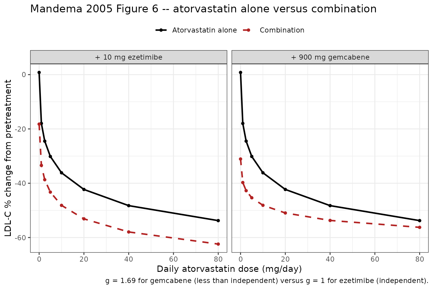

Replicates Figure 6 of Mandema 2005: atorvastatin monotherapy versus atorvastatin combined with 900 mg gemcabene (left) or 10 mg ezetimibe (right). Ezetimibe adds a roughly constant increment across the whole atorvastatin dose range; gemcabene’s increment collapses as the atorvastatin dose rises.

The pharmacological-independence identity (ezetimibe, g = 1)

The paper defines independence explicitly: “the expected LDL-C reduction can be calculated as 1 - (1 - statin fractional LDL-C reduction) * (1 - ezetimibe fractional LDL-C reduction). An independent interaction is represented in the dose-response model by an interaction coefficient g of 1.”

That is an algebraic identity the implementation must satisfy exactly for ezetimibe (whose g is held at 1), and must not satisfy for gemcabene (g = 1.69). Checking both directions confirms both the 0.01 scaling factor in Equation 1 and that the two interaction coefficients are not swapped.

grid <- c(0, 2.5, 5, 10, 20, 40, 80)

statin_only <- solve_arms(dplyr::bind_rows(lapply(grid, function(d)
  arm(CONMED_ATORVASTATIN_DOSE = d))))$pct_change_ldlc - placebo
#> Warning: multi-subject simulation without without 'omega'
ezt_only <- solve_arms(arm(CONMED_EZT_DOSE = 10))$pct_change_ldlc - placebo
gem_only <- solve_arms(arm(CONMED_GEMCABENE_DOSE = 900))$pct_change_ldlc - placebo

combo_ezt <- solve_arms(dplyr::bind_rows(lapply(grid, function(d)
  arm(CONMED_ATORVASTATIN_DOSE = d, CONMED_EZT_DOSE = 10))))$pct_change_ldlc - placebo
#> Warning: multi-subject simulation without without 'omega'
combo_gem <- solve_arms(dplyr::bind_rows(lapply(grid, function(d)
  arm(CONMED_ATORVASTATIN_DOSE = d, CONMED_GEMCABENE_DOSE = 900))))$pct_change_ldlc - placebo
#> Warning: multi-subject simulation without without 'omega'

# Independence prediction, expressed as a percentage change (negative).
independent <- function(a, b) -100 * (1 - (1 + a / 100) * (1 + b / 100))

ind_ezt <- independent(statin_only, ezt_only)
ind_gem <- independent(statin_only, gem_only)

cat(sprintf("Ezetimibe: max |model - independence identity| = %.10f %%-points\n",
            max(abs(combo_ezt - ind_ezt))))
#> Ezetimibe: max |model - independence identity| = 0.0000000000 %-points
cat(sprintf("Gemcabene: max |model - independence identity| = %.2f %%-points (should be LARGE)\n",
            max(abs(combo_gem - ind_gem))))
#> Gemcabene: max |model - independence identity| = 12.00 %-points (should be LARGE)

# Ezetimibe: exact algebraic identity, so machine precision is the right bound.
stopifnot(max(abs(combo_ezt - ind_ezt)) < 1e-8)
# Gemcabene: must be clearly sub-independent (g = 1.69, not 1). At 80 mg
# atorvastatin the model gives -2.5% additional versus -13.4% under
# independence, so this departure is not marginal.
stopifnot(max(abs(combo_gem - ind_gem)) > 5)

The ezetimibe combination reproduces the independence identity to machine precision, and the gemcabene combination departs from it by more than 10 percentage points at the top of the atorvastatin dose range. That is the paper’s central finding, restated as an assertion.

The decision the model supported

decision <- data.frame(
  Statement = c(
    "At atorvastatin 10 mg, 900 mg gemcabene and 10 mg ezetimibe add the same ~12%",
    "At atorvastatin 80 mg, gemcabene adds only ~2.5% versus ezetimibe's ~8.7%",
    "900 mg gemcabene alone is about as effective as 5 mg atorvastatin"
  ),
  Model = c(
    sprintf("gemcabene %.1f%% vs ezetimibe %.1f%%", table3$gem_model[2], table3$ezt_model[2]),
    sprintf("gemcabene %.1f%% vs ezetimibe %.1f%%", table3$gem_model[5], table3$ezt_model[5]),
    sprintf("gemcabene 900 mg %.1f%% vs atorvastatin 5 mg %.1f%%",
            gem_only,
            solve_arms(arm(CONMED_ATORVASTATIN_DOSE = 5))$pct_change_ldlc - placebo)
  )
)
knitr::kable(decision, caption = "The three quantitative claims in the Mandema 2005 Discussion that drove the decision to stop gemcabene development.")

The three quantitative claims in the Mandema 2005 Discussion that drove the decision to stop gemcabene development.

Statement	Model
At atorvastatin 10 mg, 900 mg gemcabene and 10 mg ezetimibe add the same ~12%	gemcabene -12.0% vs ezetimibe -12.0%
At atorvastatin 80 mg, gemcabene adds only ~2.5% versus ezetimibe’s ~8.7%	gemcabene -2.5% vs ezetimibe -8.6%
900 mg gemcabene alone is about as effective as 5 mg atorvastatin	gemcabene 900 mg -31.9% vs atorvastatin 5 mg -30.9%

# "about the same LDL-C reduction as 5 mg of atorvastatin" (Discussion).
ator5 <- solve_arms(arm(CONMED_ATORVASTATIN_DOSE = 5))$pct_change_ldlc - placebo
stopifnot(abs(gem_only - ator5) < 1.5)

The European placebo shift

The only retained covariate is trial location. Because it acts on the intercept E0, it shifts every arm of a European trial equally and therefore cancels out of any within-trial contrast such as Table 3. This check confirms both halves of that statement.

eu_placebo <- solve_arms(arm(REGION_EUROPE = 1))$pct_change_ldlc
eu_active  <- solve_arms(arm(REGION_EUROPE = 1, CONMED_ATORVASTATIN_DOSE = 10))$pct_change_ldlc
na_active  <- solve_arms(arm(CONMED_ATORVASTATIN_DOSE = 10))$pct_change_ldlc

cat(sprintf("Placebo arm: North America %+.3f%%, Europe %+.3f%% (shift %+.3f)\n",
            placebo, eu_placebo, eu_placebo - placebo))
#> Placebo arm: North America +0.802%, Europe -3.198% (shift -4.000)
cat(sprintf("Active-minus-placebo contrast: North America %+.4f%%, Europe %+.4f%%\n",
            na_active - placebo, eu_active - eu_placebo))
#> Active-minus-placebo contrast: North America -36.9569%, Europe -36.9569%

stopifnot(
  abs((eu_placebo - placebo) - (-4)) < 1e-8,                 # exactly -4 points
  abs((na_active - placebo) - (eu_active - eu_placebo)) < 1e-8  # cancels exactly
)

Assumptions and deviations

• No NCA / PKNCA validation. This model has no PK layer, no concentrations and no time course; it maps a per-arm daily dose directly to a per-arm mean percentage change in LDL-C. Non-compartmental analysis is not defined for it. The validation above is instead a set of deterministic replications of the paper’s own published outputs (Table 3 in full, the Discussion’s point predictions and relative potencies, and the independence identity the paper states in words). This follows the same approach as the sibling MBMA vignettes Vargo_2014_statins_ezetimibe_mbma and Mandema_2011_anticoagulants_mbma.

• Residual SD held at zero. Equation 1 declares a between-subject residual eps ~ N(0, sigma^2), but no numeric value for sigma is published anywhere in the paper – not in Table 2, not in the Results text, and there is no supplement. Rather than invent a variance, addSd is wrapped in fixed(0). The endpoint is still declared, so a downstream user can unfix and estimate it against their own data; as shipped, the model returns the typical study-arm mean exactly. Note that in the source the residual applied to a study-arm mean, so it would in any case need sample-size reweighting before being used as an individual-level error.

• Trial random effect not encoded. Equation 1 includes a trial-specific random effect eta with variance nu^2. The paper reports that this variance “was found to be not statistically significantly different from zero, suggesting homogeneity between studies,” and gives no numeric estimate. It is therefore omitted rather than encoded as a zero-variance eta, which would produce a singular OMEGA that rxode2’s Cholesky sampler cannot decompose. The sibling models Vargo_2014_statins_ezetimibe_mbma and Mandema_2011_anticoagulants_mbma treat their driven-to-zero between-trial variances the same way.

• Uncertainty bands not reproduced. The paper’s 5th/95th percentiles in Table 3 and Figure 6 come from sampling 5,000 parameter sets from the estimated variance-covariance matrix. Table 2 publishes only marginal 95% confidence intervals, not the covariance matrix, so those bands cannot be reconstructed faithfully. Only the means are validated above. Treating the marginal intervals as independent would understate the correlation between Emax and ED50 and give misleadingly wide bands.

• European placebo effect is prose-only, to one significant figure. The value -4 percentage points comes from the Results sentence “An additional 4% reduction in LDL-C was consistently observed in Europeans trials.” It has no row in Table 2 and no confidence interval. The reference category is taken to be North American (United States) trials, which is how the sentence reads (“a difference between North American and European studies … an additional 4% reduction … in European trials”) and is consistent with Table 2’s unqualified E0. Because the paper does not tabulate which trials were European, this covariate cannot be cross-checked against any published output.

• Only the LDL-C endpoint is extracted. The Abstract and Introduction also describe models for HDL-C, persistent alanine aminotransferase elevation, myalgia, headache, and coronary-artery-disease risk reduction. The paper states that “the LDL-C effect … is the main focus of this article” and publishes parameter estimates for the LDL-C dose-response only (Table 2). No parameter values for the other endpoints appear anywhere in the paper, so they cannot be extracted; this is a reporting gap in the source, not a scope decision.

• Two nonstatins written as two terms. Equation 1 has a single Enonstatin and a single g because the paper only ever combined a statin with one nonstatin. The model file writes out one term per nonstatin, each with its own interaction coefficient. For every arm the paper actually studied this reduces exactly to Equation 1. An arm coding both ezetimibe and gemcabene at once would add their effects with no ezetimibe-gemcabene interaction term – a combination the paper never studied and did not parameterise.

• Statin selection by summed potency ratio. Equation 2 is Dose^n * Emax / (Dose^n + ED50^n), which is identically Emax * ratio^n / (ratio^n + 1) for a potency-normalised dose ratio = Dose / ED50. Since the five statins share Emax and n, the model sums those potency-normalised doses across statins. Every trial arm in Table 1 contains at most one statin, so exactly one term is non-zero and this is exact. Coding two statins simultaneously is outside the paper’s calibration range.

• Species and population. Human. The pooled cohort is predominantly adults with hypercholesterolemia, but three of the four gemcabene trials enrolled healthy volunteers, healthy obese subjects, or subjects with low HDL-C; their much lower baseline LDL-C was adjusted for by an upstream ANOVA before the arm means entered this dose-response model, so that adjustment is baked into the source data rather than into the model equations.