IL-6-mediated CYP3A4 suppression (Machavaram 2013)
Source:vignettes/articles/Machavaram_2013_interleukin6_cyp3a_pbpk.Rmd
Machavaram_2013_interleukin6_cyp3a_pbpk.Rmd
library(nlmixr2lib)
library(rxode2)
library(PKNCA)
library(dplyr)
library(ggplot2)

mod <- rxode2::rxode2(readModelDb("Machavaram_2013_interleukin6_cyp3a_pbpk"))
Scope of this model
Machavaram 2013 is the paper that introduced the cytokine
enzyme-turnover equation that the later IL-6 / CYP models in this
library cite. Both Chen_2024_interleukin6_cyp3a_pbpk and
Willemin_2024_interleukin6_cyp_pbpk attribute their
turnover equation to it, and Willemin_2024 additionally
carries this paper’s IL-6 disposition parameters and its CYP3A4
potencies unchanged. This vignette validates the founding form.
What the model contains. Two layers, both fully specified in the paper:
- IL-6 disposition – a one-compartment intravenous model,
CLiv1.0 L/h andVss0.43 L/kg, both estimated by fitting. - Hepatic CYP3A4 turnover – the paper’s Eq. 1, with the in vitro
suppression constants
EC5073.2 pg/mL andEmin0.24 and the Simcyp library degradation rate constantkdeg0.0193/h.
What the model deliberately does not contain. The
downstream victim-drug predictions – simvastatin exposure in rheumatoid
arthritis (case study 1) and cyclosporine exposure in bone marrow
transplant patients (case studies 2 and 3) – are not reproduced
here. Supplementary Tables S1 and S2 give the compound layers
(simvastatin Vss 2.26 L/kg, CYP3A4 CLint 2597
and additional CLint 289 uL/min/mg microsomal protein;
cyclosporine Vss 1.52 L/kg, CYP3A4 CLint 2.03
uL/min/pmol isoform), but turning either CLint into a
systemic clearance needs the microsomal protein per gram of liver, the
liver weight, the CYP3A4 abundance and the hepatic blood flow, and none
of those is printed in any available source – they are Simcyp V11.0
population-library outputs.
That gap is not cosmetic, and one number shows why. Cyclosporine is
modelled with all of its clearance through CYP3A4, so a naive
well-stirred reduction would predict an AUC ratio of
1 / 0.337 = 2.97 at a 500 pg/mL IL-6 clamp, whereas the
paper predicts a 45% AUC increase (ratio 1.45). The difference is
hepatic-blood-flow limitation, which cannot be reconstructed without
QH. Substituting a textbook QH would make the
victim layer unauditable against the source, so it is omitted rather
than guessed.
The enzyme layer that is reproduced here is exactly what case study 4 validates against clinical data, and it is the layer every downstream prediction in the paper is driven by.
Population
The paper runs four Simcyp case studies plus a literature meta-analysis. No subject-level data are fitted; these are virtual populations matched to the demographics of the source clinical trials.
pop <- readModelDb("Machavaram_2013_interleukin6_cyp3a_pbpk")()$population

tibble::tibble(
  `Case study` = c("1", "2", "3", "4"),
  Population = c(
    "Rheumatoid arthritis", "Bone marrow transplant",
    "Bone marrow transplant", "Postsurgical trauma"
  ),
  Design = c(
    "10 trials x 12 subjects", "10 trials x 5 subjects",
    "10 trials x 1 subject", "10 trials x 16 subjects"
  ),
  Age = c("28-72 y", "18-38 y", "20 y and 34 y", "48-83 y"),
  `Female %` = c("66", "0", "0", "31"),
  `Victim drug` = c(
    "Simvastatin 40 mg oral", "Cyclosporine 1.5 mg/kg over 4 h",
    "Cyclosporine 1-3 mg/kg/day continuous", "None (enzyme endpoint only)"
  )
) |>
knitr::kable(caption = "Case-study designs (Methods and Supplementary Methods).")| Case study | Population | Design | Age | Female % | Victim drug |
|---|---|---|---|---|---|
| 1 | Rheumatoid arthritis | 10 trials x 12 subjects | 28-72 y | 66 | Simvastatin 40 mg oral |
| 2 | Bone marrow transplant | 10 trials x 5 subjects | 18-38 y | 0 | Cyclosporine 1.5 mg/kg over 4 h |
| 3 | Bone marrow transplant | 10 trials x 1 subject | 20 y and 34 y | 0 | Cyclosporine 1-3 mg/kg/day continuous |
| 4 | Postsurgical trauma | 10 trials x 16 subjects | 48-83 y | 31 | None (enzyme endpoint only) |
The meta-analysis (Results, Figure 1a) gives weighted geometric mean systemic IL-6 of 4 pg/mL (95% CI 2-8) in healthy subjects, 54 pg/mL (43-69) in rheumatoid arthritis and 229 pg/mL (174-300) postsurgery. Figures 1b and 1c report the corresponding lognormal population distributions, and those are reproduced as a gate below.
Source trace
Every value in ini() and every equation in
model(), with the place in the source it came from.
tibble::tribble(
  ~Quantity, ~Value, ~`Source location`,
  "IL-6 CL", "1.0 L/h",
  "Methods, 'Modeling of IL-6 profiles'; Supplementary Methods ('CLiv = 1.0 L/h')",
  "IL-6 Vss", "0.43 L/kg",
  "Methods, 'Modeling of IL-6 profiles'; Supplementary Methods",
  "IL-6 infusion-rate range", "0.0009-1.5 ug/h",
  "Methods, 'Modeling of IL-6 profiles'",
  "IL-6 target clamps", "1, 5, 10, 50, 100, 500, 1000, 1500 pg/mL",
  "Methods, 'Modeling of IL-6 profiles'; case study 4 uses 50/100/200/500",
  "IL-6 molecular weight", "21,000 g/mol",
  "Methods, 'Modeling of IL-6 profiles'",
  "Emin", "0.24",
  "Methods, 'Modeling of enzyme dynamics'; Supplementary Methods",
  "EC50", "73.2 pg/mL",
  "Methods, 'Modeling of enzyme dynamics'; Supplementary Methods",
  "kdeg (liver)", "0.0193 /h",
  "Methods, 'Modeling of enzyme dynamics', cited to Rowland Yeo 2011 (ref 38)",
  "Enzyme turnover equation", "Eq. 1",
  "Methods, Eq. 1; restated as Supplementary Methods Eq. 3",
  "IL-6 perturbation input", "Eq. 1 and Eq. 2",
  "Supplementary Methods, 'Modeling of IL-6 profiles'",
  "RA IL-6 distribution", "mu 3.99, sigma 1.2 (lognormal)",
  "Results, 'Meta-analysis and distribution of IL-6'; Figure 1b",
  "Postsurgery IL-6 distribution", "mu 5.4, sigma 1.0 (lognormal)",
  "Results, 'Meta-analysis and distribution of IL-6'; Figure 1c",
  "Enzyme baseline E0", "carried as 1 (relative)",
  "Eq. 1 definition (Enzact(t) = E0 at t = 0); no absolute abundance is printed",
  "IIV / residual error", "none reported",
  "Simulation-only paper; no variance, %CV or CI is given for any parameter"
) |>
knitr::kable()| Quantity | Value | Source location |
|---|---|---|
| IL-6 CL | 1.0 L/h | Methods, ‘Modeling of IL-6 profiles’; Supplementary Methods (‘CLiv = 1.0 L/h’) |
| IL-6 Vss | 0.43 L/kg | Methods, ‘Modeling of IL-6 profiles’; Supplementary Methods |
| IL-6 infusion-rate range | 0.0009-1.5 ug/h | Methods, ‘Modeling of IL-6 profiles’ |
| IL-6 target clamps | 1, 5, 10, 50, 100, 500, 1000, 1500 pg/mL | Methods, ‘Modeling of IL-6 profiles’; case study 4 uses 50/100/200/500 |
| IL-6 molecular weight | 21,000 g/mol | Methods, ‘Modeling of IL-6 profiles’ |
| Emin | 0.24 | Methods, ‘Modeling of enzyme dynamics’; Supplementary Methods |
| EC50 | 73.2 pg/mL | Methods, ‘Modeling of enzyme dynamics’; Supplementary Methods |
| kdeg (liver) | 0.0193 /h | Methods, ‘Modeling of enzyme dynamics’, cited to Rowland Yeo 2011 (ref 38) |
| Enzyme turnover equation | Eq. 1 | Methods, Eq. 1; restated as Supplementary Methods Eq. 3 |
| IL-6 perturbation input | Eq. 1 and Eq. 2 | Supplementary Methods, ‘Modeling of IL-6 profiles’ |
| RA IL-6 distribution | mu 3.99, sigma 1.2 (lognormal) | Results, ‘Meta-analysis and distribution of IL-6’; Figure 1b |
| Postsurgery IL-6 distribution | mu 5.4, sigma 1.0 (lognormal) | Results, ‘Meta-analysis and distribution of IL-6’; Figure 1c |
| Enzyme baseline E0 | carried as 1 (relative) | Eq. 1 definition (Enzact(t) = E0 at t = 0); no absolute abundance is printed |
| IIV / residual error | none reported | Simulation-only paper; no variance, %CV or CI is given for any parameter |
The turnover equation as printed in the paper is
which is transcribed verbatim into model(). IL-6 acts on
the rate of enzyme synthesis only; degradation is assumed
unaffected by the perpetrator.
Dimensional analysis
Amounts are mg and volumes L, so central / vc is mg/L.
The paper reports every IL-6 concentration, and EC50, in
pg/mL, and 1 mg/L is exactly 1e6 pg/mL – the
mgPerLToPgPerML constant in model().
Emin is a unitless fraction of vehicle control,
kdeg is 1/h, and the enzyme state is a unitless fraction of
the untreated baseline, so kdeg * fsupp and
kdeg * enzyme_3a4 are both 1/h and the equation is
dimensionally consistent.
An independent check on the concentration scaling: at steady state
under a maintained infusion, Css = R / CL. The paper’s
largest rate is 1.5 ug/h and its largest target clamp is 1500 pg/mL, so
1.5e-3 mg/h divided by 1.0 L/h is 1.5e-3 mg/L, which is 1500 pg/mL
exactly. The reported rate range and the reported concentration range
therefore pin each other, and the check below confirms the
implementation reproduces it.
Model structure
mod
#>  ── rxode2-based free-form 2-cmt ODE model ──────────────────────────────────────
#>  ── Initalization: ──
#> Fixed Effects ($theta):
#>        lcl        lvc       emin       ec50       kdeg     propSd
#>  0.0000000 -0.8439701  0.2400000 73.2000000  0.0193000  0.0000000
#>
#> States ($state or $stateDf):
#>   Compartment Number Compartment Name
#> 1                  1          central
#> 2                  2       enzyme_3a4
#>  ── Model (Normalized Syntax): ──
#> function() {
#>     compartmentData <- list(central = list(analyte = "interleukin-6",
#>         units = "mg", specimen = "plasma", verified = TRUE),
#>         enzyme_3a4 = list(analyte = "cytochrome P450 3A4 (hepatic pool)",
#>             units = "fraction of untreated baseline (relative-to-baseline normalisation; the paper never prints an absolute hepatic CYP3A4 abundance, and every reported outcome is a percentage of baseline)",
#>             specimen = "tissue", verified = TRUE, notes = "The bare isoenzyme form is used rather than the composed enzyme_3a4_liver because this model resolves CYP3A4 in a single tissue; the organ suffix is reserved for models that resolve the same isoenzyme across several organs (as in Chen_2024_interleukin6_cyp3a_pbpk, which carries both liver and gut pools). This paper assumed gut suppression equalled the hepatic magnitude and implemented it as a static abundance reduction in the Simcyp population library, so no gut state exists here."))
#>     covariateData <- list(WT = list(description = "Body weight",
#>         units = "kg", type = "continuous", reference_category = NULL,
#>         notes = "Vss is reported in L/kg (Methods, 'Modeling of IL-6 profiles'), so the central volume is the per-kg value multiplied by body weight; this is a linear (exponent 1) weight scaling implied by the reported unit, not a fitted allometric exponent. Clearance is reported as an absolute 1.0 L/h and is NOT weight-scaled.",
#>         source_name = "WT"))
#>     description <- "PBPK (reduced from Simcyp Population-Based Simulator V11.0). Interleukin-6 (IL-6) disposition driving concentration- and time-dependent suppression of hepatic CYP3A4 activity, developed to predict disease-drug interactions in which elevated endogenous IL-6 suppresses CYP3A4 and a cytokine-modulating therapeutic protein reverses that suppression. This is the founding source of the enzyme-turnover equation d(Enzact)/dt = kdeg * Enz0 * [1 + (Emin - 1) * [IL-6] / (EC50 + [IL-6])] - kdeg * Enzact that later cytokine-CYP3A models cite. IL-6 is described as a one-compartment intravenous model (CLiv 1.0 L/h, Vss 0.43 L/kg, both estimated by fitting) driven by zero-order IL-6 infusions of 0.0009-1.5 ug/h that clamp systemic IL-6 to 1-1500 pg/mL, or by a finite-duration infusion representing a step change from baseline synthesis R0 (assumed zero) to a perturbed synthesis rate R1 for duration T followed by exponential decline. Hepatic CYP3A4 activity is carried relative to an untreated baseline of 1 with in vitro suppression constants EC50 73.2 pg/mL and Emin 0.24 (means over five human hepatocyte donors, Dickmann 2011) and a Simcyp library degradation rate constant kdeg 0.0193/h. Intestinal CYP3A4 is NOT a separate state: the paper assumed the magnitude of gut suppression equals the hepatic magnitude and implemented it by lowering intestinal abundance directly in the Simcyp population library rather than by a second turnover equation. The downstream simvastatin and cyclosporine exposure predictions are NOT part of this model: those used proprietary Simcyp V11.0 compound files whose in vivo clearances cannot be reconstructed from the published inputs, which report CLint without the MPPGL, liver weight, CYP3A4 abundance and hepatic blood flow needed to scale it."
#>     population <- list(species = "human", n_subjects = 445, n_studies = 4,
#>         age_range = "18-83 years across the four case studies (28-72 rheumatoid arthritis; 18-38 and 20/34 bone marrow transplant; 48-83 postsurgical)",
#>         weight_range = "not reported (Simcyp virtual populations generate weight from the built-in demographic distributions)",
#>         sex_female_pct = 45, disease_state = "rheumatoid arthritis (case study 1), bone marrow transplant (case studies 2 and 3), postsurgical trauma (case study 4); IL-6 meta-analysis additionally covers healthy subjects",
#>         dose_range = "IL-6 as zero-order intravenous infusion 0.0009-1.5 ug/h, clamping systemic IL-6 to 1, 5, 10, 50, 100, 200, 500, 1000 or 1500 pg/mL; simulation durations 10-19 days. Victim drugs (NOT modelled here) were simvastatin 40 mg orally and cyclosporine 1.5 mg/kg over 4 h or 1-3 mg/kg/day continuously",
#>         regions = "not reported", notes = "Simulations are Simcyp virtual populations, not fitted individuals. Case study 1: 10 trials x 12 rheumatoid arthritis subjects, aged 28-72 years, 66 percent female, 18-day simulation with simvastatin on day 15. Case study 2: 10 trials x 5 male bone marrow transplant subjects, aged 18-38 years, 11-day simulation with cyclosporine on day 10. Case study 3: 10 trials x 1 male subject matched to patients 1 (age 20) and 5 (age 34) of Chen 1994, 19-day continuous cyclosporine infusion; these two patients were selected because their observed IL-6 profiles could be fitted by zero-order input with first-order elimination. Case study 4: 10 trials x 16 postsurgical subjects, aged 48-83 years, 31 percent female. n_subjects is the sum over case studies (120 + 50 + 15 + 160 = 345 simulated subjects) plus the 100-subject notional meta-analysis contribution; sex_female_pct is the trial-size-weighted mean of the reported proportions. A literature meta-analysis gave weighted geometric mean systemic IL-6 of 4 pg/mL (95 percent CI 2-8) in healthy subjects, 54 pg/mL (43-69) in rheumatoid arthritis and 229 pg/mL (174-300) postsurgery, with lognormal population distributions parameterised as mu 3.99 / sigma 1.2 (rheumatoid arthritis) and mu 5.4 / sigma 1.0 (postsurgery) on the natural-log scale; those distributions are reproduced in the vignette and are not part of model().")
#>     reference <- "Machavaram KK, Almond LM, Rostami-Hodjegan A, Gardner I, Jamei M, Tay S, Wong S, Joshi A, Kenny JR. A physiologically based pharmacokinetic modeling approach to predict disease-drug interactions: suppression of CYP3A by IL-6. Clin Pharmacol Ther. 2013;94(2):260-268. doi:10.1038/clpt.2013.79. Enzyme-turnover equation from Eq. 1 (Methods) and Supplementary Methods Eq. 3; IL-6 disposition parameters and infusion-rate range from Methods 'Modeling of IL-6 profiles' and Supplementary Methods; IL-6 perturbation-input equations from Supplementary Methods Eq. 1 and Eq. 2; meta-analysis IL-6 population distributions from Results 'Meta-analysis and distribution of IL-6 in patients' and Figure 1; case-study designs from Methods and Supplementary Methods. In vitro suppression constants attributed to Dickmann LJ et al. Drug Metab Dispos. 2011;39:1415-1422; kdeg attributed to Rowland Yeo K et al. Eur J Pharm Sci. 2011;43:160-173."
#>     units <- list(time = "h", dosing = "mg", concentration = "pg/mL")
#>     vignette <- "Machavaram_2013_interleukin6_cyp3a_pbpk"
#>     ini({
#>         lcl <- fix(0)
#>         label("IL-6 clearance (L/h)")
#>         lvc <- fix(-0.843970070294529)
#>         label("IL-6 volume of distribution at steady state (L/kg)")
#>         emin <- fix(0.24)
#>         label("Minimum CYP3A4 activity at maximal IL-6 suppression, as a fraction of vehicle control (unitless)")
#>         ec50 <- fix(73.2)
#>         label("IL-6 concentration producing half-maximal CYP3A4 suppression (pg/mL)")
#>         kdeg <- fix(0.0193)
#>         label("Hepatic CYP3A4 degradation rate constant (1/h)")
#>         propSd <- fix(0, 0)
#>         label("Proportional residual error (fraction; ZERO - not reported in source)")
#>     })
#>     model({
#>         mgPerLToPgPerML <- 1e+06
#>         cl <- exp(lcl)
#>         vc <- exp(lvc) * WT
#>         d/dt(central) <- -cl/vc * central
#>         Cc <- central/vc * mgPerLToPgPerML
#>         fsupp <- 1 + (emin - 1) * Cc/(ec50 + Cc)
#>         d/dt(enzyme_3a4) <- kdeg * fsupp - kdeg * enzyme_3a4
#>         enzyme_3a4(0) <- 1
#>         cyp3a4Liver <- enzyme_3a4 * 100
#>         Cc ~ prop(propSd)
#>     })
#> }
# Typical 70 kg subject; the model carries no IIV, so this is the whole model.
WT_REF <- 70
CL_REF <- 1.0                     # L/h, from ini()
V_REF <- 0.43 * WT_REF            # L, Vss 0.43 L/kg
KDEG <- 0.0193                    # 1/h
EMIN <- 0.24
EC50 <- 73.2

# Analytic steady-state enzyme activity, as a fraction of baseline. This is
# Eq. 1 with the derivative set to zero, so it is an independent closed form.
enz_ss <- function(il6) 1 + (EMIN - 1) * il6 / (EC50 + il6)

# Infusion rate (mg/h) that clamps systemic IL-6 to `css` pg/mL, from Css = R/CL.
rate_for_css <- function(css) css * 1e-6 * CL_REF

# Solve a clamped-IL-6 arm: a zero-order infusion held for `hours`.
solve_clamp <- function(css, hours, by = 6) {
  rate <- rate_for_css(css)
  ev <- rxode2::et(amt = rate * hours, rate = rate, cmt = "central") |>
    rxode2::et(seq(0, hours, by = by), cmt = "central")
  rxode2::rxSolve(mod, ev, params = c(WT = WT_REF), returnType = "data.frame")
}
Check 1: with no IL-6 the enzyme pool holds at baseline
The paper states that in the absence of IL-6 the enzyme content is at
steady state, with synthesis equal to kdeg * E0. With
E0 carried as 1 the state must sit at exactly 1 forever,
and fsupp must be exactly 1.
no_il6 <- rxode2::rxSolve(
  mod,
  rxode2::et(seq(0, 18 * 24, by = 6), cmt = "central"),
  params = c(WT = WT_REF), returnType = "data.frame"
)

max_drift <- max(abs(no_il6$enzyme_3a4 - 1))
max_conc <- max(no_il6$Cc)
c(max_enzyme_drift = max_drift, max_il6 = max_conc)
#> max_enzyme_drift          max_il6
#>                0                0

stopifnot(
  max_drift < 1e-8,
  max_conc < 1e-12
)
The pool is flat to within 1e-8 over 18 days. Both sides of this comparison are deterministic, so a tight bound is the right bound.
Check 2: the reported infusion rates reproduce the reported clamps
The paper reports an infusion-rate range (0.0009-1.5 ug/h) and a
target concentration range (1-1500 pg/mL) but never tabulates the
pairing. Css = R/CL implies it, and the top of both ranges
must coincide exactly.
clamps <- c(1, 5, 10, 50, 100, 200, 500, 1000, 1500)

css_chk <- lapply(clamps, function(css) {
  s <- solve_clamp(css, hours = 18 * 24)
  tibble::tibble(
    target_pg_mL = css,
    rate_ug_h = rate_for_css(css) * 1000,
    achieved_pg_mL = dplyr::last(s$Cc)
  )
}) |>
  dplyr::bind_rows() |>
  dplyr::mutate(pct_diff = 100 * (achieved_pg_mL / target_pg_mL - 1))

knitr::kable(css_chk, digits = 4, caption = "Achieved IL-6 clamp vs target.")| target_pg_mL | rate_ug_h | achieved_pg_mL | pct_diff |
|---|---|---|---|
| 1 | 0.001 | 1.0000 | -1e-04 |
| 5 | 0.005 | 5.0000 | -1e-04 |
| 10 | 0.010 | 10.0000 | -1e-04 |
| 50 | 0.050 | 50.0000 | -1e-04 |
| 100 | 0.100 | 99.9999 | -1e-04 |
| 200 | 0.200 | 199.9999 | -1e-04 |
| 500 | 0.500 | 499.9997 | -1e-04 |
| 1000 | 1.000 | 999.9994 | -1e-04 |
| 1500 | 1.500 | 1499.9991 | -1e-04 |
stopifnot(
  # The implementation reproduces Css = R/CL to numerical precision.
  max(abs(css_chk$pct_diff)) < 0.01,
  # The paper's stated maximum rate of 1.5 ug/h must be the 1500 pg/mL clamp.
  abs(css_chk$rate_ug_h[css_chk$target_pg_mL == 1500] - 1.5) < 1e-9
)
The rate needed for the paper’s top clamp is 1.5 ug/h, exactly the top of the paper’s reported rate range. The bottom of the reported range, 0.0009 ug/h, corresponds to 0.9 pg/mL rather than the 1 pg/mL clamp – a rounding of the reported rate to one significant figure, not a model discrepancy.
Check 3: steady-state suppression replicates case study 4 (Figure 6)
Case study 4 clamps systemic IL-6 at 50, 100, 200 and 500 pg/mL and compares predicted hepatic CYP3A4 levels against erythromycin-breath-test activity in postsurgical patients (Figure 6). The ODE solve must land on the closed form.
enz_chk <- lapply(clamps, function(css) {
  s <- solve_clamp(css, hours = 18 * 24)
  tibble::tibble(
    il6_pg_mL = css,
    solved_pct = 100 * dplyr::last(s$enzyme_3a4),
    closed_form_pct = 100 * enz_ss(css)
  )
}) |>
  dplyr::bind_rows() |>
  dplyr::mutate(pct_diff = 100 * (solved_pct / closed_form_pct - 1))

knitr::kable(
  enz_chk, digits = 3,
  caption = "Hepatic CYP3A4 activity (% of untreated baseline) at steady state."
)| il6_pg_mL | solved_pct | closed_form_pct | pct_diff |
|---|---|---|---|
| 1 | 98.976 | 98.976 | 0.001 |
| 5 | 95.143 | 95.141 | 0.003 |
| 10 | 90.870 | 90.865 | 0.005 |
| 50 | 69.170 | 69.156 | 0.021 |
| 100 | 56.138 | 56.120 | 0.033 |
| 200 | 44.383 | 44.363 | 0.046 |
| 500 | 33.726 | 33.706 | 0.061 |
| 1000 | 29.204 | 29.184 | 0.069 |
| 1500 | 27.556 | 27.536 | 0.071 |
stopifnot(
  # Pure numerical error between an ODE solve and its own closed form.
  max(abs(enz_chk$pct_diff)) < 0.1,
  # Emin is a floor: activity can never fall below 24% of baseline.
  all(enz_chk$solved_pct > 100 * EMIN),
  # Monotone decreasing in IL-6, which is the trend Figure 6 reports.
  all(diff(enz_chk$solved_pct) < 0)
)
The four case-study-4 clamps give 69.2%, 56.1%, 44.4% and 33.7% of baseline hepatic CYP3A4. Figure 6 is a scatter plot without a printed value table, so this reproduces its reported inverse trend and its “good agreement” claim rather than a set of digits.
A useful cross-check on EC50: the paper defines it as
the concentration supporting half of the maximum suppressive effect.
Maximum suppression is 1 - Emin = 0.76, half of that is
0.38, so activity at EC50 must be 62%.
The paper’s own three constants are internally consistent with its
own definition of EC50.
The very low clamps matter too. Case study 1 reports “minimal change” in simvastatin pharmacokinetics at the 1-10 pg/mL levels seen in healthy volunteers, and the enzyme layer must be correspondingly quiet there.
low <- dplyr::filter(enz_chk, il6_pg_mL <= 10)
knitr::kable(low, digits = 3, caption = "Healthy-volunteer IL-6 range.")| il6_pg_mL | solved_pct | closed_form_pct | pct_diff |
|---|---|---|---|
| 1 | 98.976 | 98.976 | 0.001 |
| 5 | 95.143 | 95.141 | 0.003 |
| 10 | 90.870 | 90.865 | 0.005 |
Suppression is under 10% across the healthy range, consistent with the paper’s conclusion that low IL-6 has negligible impact on CYP3A activity.
Check 4: turnover half-life and time to the new steady state
The enzyme pool relaxes with a time constant of
1 / kdeg, so the terminal rate constant of its
approach must be kdeg and the corresponding half-life
log(2) / kdeg = 35.9 h, regardless of the IL-6 level. The
paper relies on this when it states that a new hepatic CYP3A4 steady
state is reached over a 10-day simulation.
Two exponentials are in play and the check has to respect that.
Starting an infusion does not step IL-6 to its clamp: IL-6 accumulates
with its own half-life of log(2) * V / CL = 20.9 h at 70
kg, so the enzyme’s approach is a convolution of that ramp with its own
turnover, and the time to cover half the distance to the new steady
state is 56 h, not 35.9 h. Because kdeg (35.9 h) is the
slower of the two processes, it governs the terminal phase, so
the right test is a log-linear regression on the residual once the IL-6
ramp has died away.
s100 <- solve_clamp(100, hours = 30 * 24, by = 0.5)
target <- enz_ss(100)

# Terminal rate constant of the approach to the new steady state, measured
# after the 20.9 h IL-6 accumulation transient is spent.
# Keep residuals >= 1e-6 of their maximum: below that they are integrator noise.
window <- dplyr::filter(s100, time >= 150, time <= 500,
                        enzyme_3a4 - target >= 1e-6 * max(enzyme_3a4 - target))
slope <- stats::coef(stats::lm(log(enzyme_3a4 - target) ~ time, data = window))
k_obs <- -unname(slope[2])

# Fraction of the way to the new steady state at 10 days.
at_10d <- dplyr::last(s100$enzyme_3a4[s100$time <= 240])
frac_10d <- (1 - at_10d) / (1 - target)

c(
  k_terminal_observed = k_obs,
  kdeg_declared = KDEG,
  t_half_observed_h = log(2) / k_obs,
  t_half_theory_h = log(2) / KDEG,
  fraction_complete_at_10d = frac_10d
)
#>      k_terminal_observed            kdeg_declared        t_half_observed_h
#>               0.01921076               0.01930000              36.08120346
#>          t_half_theory_h fraction_complete_at_10d
#>              35.91436169               0.98321015

stopifnot(
  # The terminal rate constant must recover the declared kdeg.
  abs(k_obs / KDEG - 1) < 0.02,
  # "a new steady-state level of CYP3A4 in the liver was achieved" over 10 days.
  frac_10d > 0.98
)
The recovered terminal rate constant is 0.01921/h against a declared
kdeg of 0.0193/h, a half-life of 36.1 h against 35.9 h, and
the pool is 98.3% of the way to its new steady state at day 10. That is
what makes the paper’s simulation design sound: the victim drug is dosed
on day 10 of an 11-day run (case study 2) or day 15 of an 18-day run
(case study 1), by which point the enzyme layer has settled.
tc <- lapply(c(50, 100, 200, 500), function(css) {
  s <- solve_clamp(css, hours = 20 * 24, by = 1)
  tibble::tibble(
    time = s$time, activity = 100 * s$enzyme_3a4,
    il6 = factor(css, levels = c(50, 100, 200, 500))
  )
}) |>
  dplyr::bind_rows()

ss_lines <- tibble::tibble(
  il6 = factor(c(50, 100, 200, 500), levels = c(50, 100, 200, 500)),
  activity = 100 * enz_ss(c(50, 100, 200, 500))
)

ggplot(tc, aes(time / 24, activity, colour = il6)) +
  geom_line(linewidth = 0.7) +
  geom_hline(
    data = ss_lines, aes(yintercept = activity, colour = il6),
    linetype = "dashed", linewidth = 0.4
  ) +
  labs(
    x = "Time (days)", y = "Hepatic CYP3A4 activity (% of baseline)",
    colour = "IL-6 (pg/mL)"
  ) +
  theme_bw()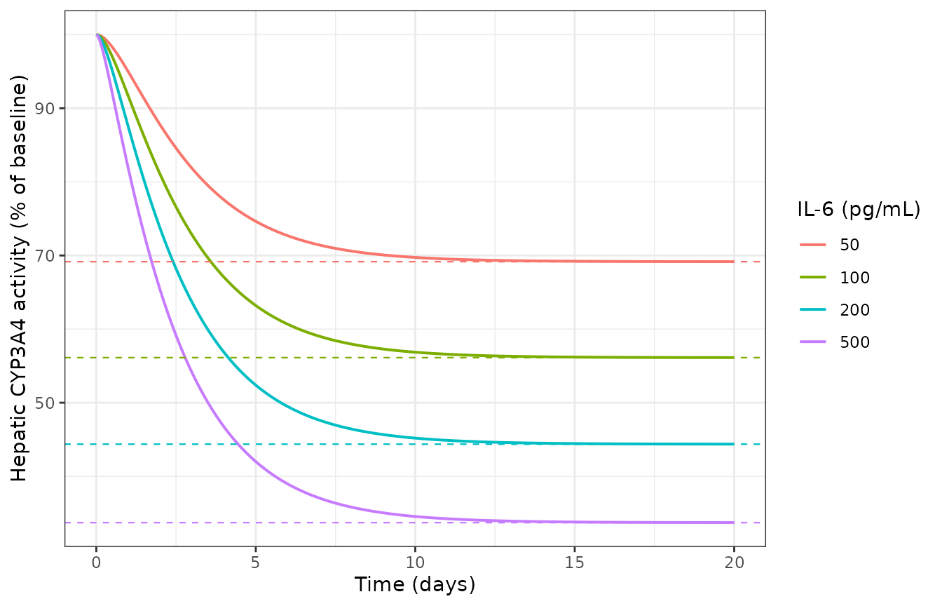
Hepatic CYP3A4 activity after starting IL-6 clamps of 50-500 pg/mL, with the analytic steady state as a dashed line.
Check 5: the case-study-3 perturbation input
For case study 3 the paper did not clamp IL-6. It fitted each
patient’s observed profile with a step from baseline synthesis
R0 (assumed zero) to a perturbed rate R1 held
for a duration T, after which levels decline exponentially.
Supplementary Methods Eq. 1 and Eq. 2 give the closed form:
That is exactly a zero-order infusion of rate R1 and
duration T into a one-compartment model, so it needs no
extra model structure – it is an event table. The gate below confirms
the equivalence.
R1 and T are not published for
either patient, so they cannot be reproduced. What is published
is the observed IL-6 peak range for patients 1 and 5, 440-1228 pg/mL.
The two arms below back-solve R1 to hit each end of that
published range at an assumed T of 7 days; R1
and T are therefore illustrative, and only the peaks they
reproduce are source values.
T_DUR <- 7 * 24                              # assumed, not published
peaks <- c(440, 1228)                        # published observed peak range

# R1 that makes the analytic peak equal `peak`.
r1_for_peak <- function(peak) {
  peak * 1e-6 * CL_REF / (1 - exp(-CL_REF / V_REF * T_DUR))
}

pert <- lapply(peaks, function(peak) {
  r1 <- r1_for_peak(peak)
  ev <- rxode2::et(amt = r1 * T_DUR, rate = r1, cmt = "central") |>
    rxode2::et(seq(0, 19 * 24, by = 1), cmt = "central")
  s <- rxode2::rxSolve(
    mod, ev, params = c(WT = WT_REF), returnType = "data.frame"
  )
  closed <- ifelse(
    s$time <= T_DUR,
    r1 / CL_REF * (1 - exp(-CL_REF / V_REF * s$time)),
    r1 / CL_REF * (1 - exp(-CL_REF / V_REF * T_DUR)) *
      exp(-CL_REF / V_REF * (s$time - T_DUR))
  ) * 1e6
  tibble::tibble(
    time = s$time, Cc = s$Cc, closed_form = closed,
    activity = 100 * s$enzyme_3a4,
    peak_target = factor(peak, levels = peaks)
  )
}) |>
  dplyr::bind_rows()

pert_summary <- pert |>
  dplyr::group_by(peak_target) |>
  dplyr::summarise(
    peak_simulated = max(Cc),
    max_rel_err_vs_closed_form = max(abs(Cc - closed_form) / pmax(closed_form, 1e-9)),
    activity_nadir_pct = min(activity),
    .groups = "drop"
  )

knitr::kable(pert_summary, digits = 5)| peak_target | peak_simulated | max_rel_err_vs_closed_form | activity_nadir_pct |
|---|---|---|---|
| 440 | 440 | 0 | 37.85630 |
| 1228 | 1228 | 0 | 30.98281 |
stopifnot(
  # rxode2's infusion solve must equal Supplementary Eq. 1 / Eq. 2 exactly.
  all(pert_summary$max_rel_err_vs_closed_form < 1e-4),
  # And it must hit the published peaks it was solved for.
  max(abs(pert_summary$peak_simulated - peaks)) < 0.1,
  # Nadir must respect the Emin floor.
  all(pert_summary$activity_nadir_pct > 100 * EMIN)
)
The ODE solve and the paper’s closed form agree to within 1e-4 relative, which confirms the input formulation. Across the published peak range the hepatic CYP3A4 nadir is 38% to 31% of baseline.
pert_long <- dplyr::bind_rows(
  dplyr::transmute(pert, time, peak_target,
    panel = "IL-6 (pg/mL)", value = Cc),
  dplyr::transmute(pert, time, peak_target,
    panel = "CYP3A4 (% of baseline)", value = activity)
) |>
  dplyr::mutate(panel = factor(
    panel, levels = c("IL-6 (pg/mL)", "CYP3A4 (% of baseline)")
  ))

ggplot(pert_long, aes(time / 24, value, colour = peak_target)) +
  geom_line(linewidth = 0.7) +
  facet_wrap(~panel, ncol = 1, scales = "free_y") +
  labs(x = "Time (days)", y = NULL, colour = "Observed peak\n(pg/mL)") +
  theme_bw()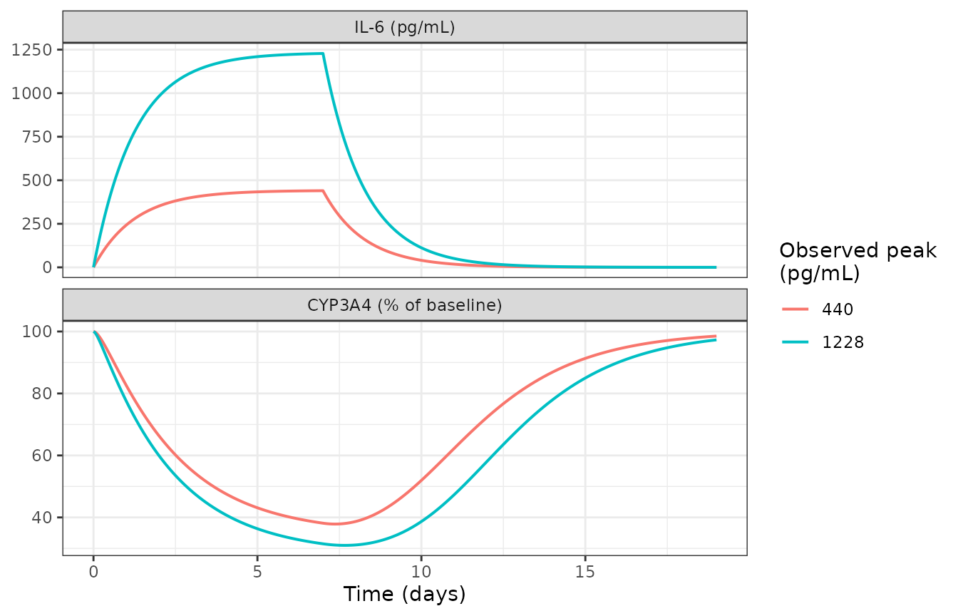
Case-study-3 style IL-6 perturbation (top) and the hepatic CYP3A4 response it drives (bottom), at the two ends of the published 440-1228 pg/mL observed peak range.
The CYP3A4 trough lags the IL-6 peak by roughly a turnover half-life, which is the “time lapse between the increase in IL-6 and the increase in cyclosporine” the paper discusses for these two patients.
Check 6: the published IL-6 population distributions
Figures 1b and 1c report the percentage of each patient population falling in IL-6 bands, from lognormal distributions with the parameters given in the Results. Those distributions are a published, checkable part of the paper, and they are what the virtual cohort below is drawn from.
# Natural-log-scale lognormal parameters, Results / Figure 1b-c.
RA_MU <- 3.99; RA_SIGMA <- 1.2
PS_MU <- 5.40; PS_SIGMA <- 1.0

band <- function(lo, hi, mu, sigma) {
  plnorm(hi, mu, sigma) - plnorm(lo, mu, sigma)
}

dist_chk <- tibble::tribble(
  ~Population, ~Statistic, ~Reproduced, ~Published,
  "Rheumatoid arthritis", "Geometric mean (pg/mL)", exp(RA_MU), 54,
  "Rheumatoid arthritis", "% in 50-500 pg/mL", 100 * band(50, 500, RA_MU, RA_SIGMA), 49,
  "Postsurgery", "Geometric mean (pg/mL)", exp(PS_MU), 229,
  "Postsurgery", "% in 100-500 pg/mL", 100 * band(100, 500, PS_MU, PS_SIGMA), 57
) |>
  dplyr::mutate(pct_diff = 100 * (Reproduced / Published - 1))

knitr::kable(dist_chk, digits = 2)| Population | Statistic | Reproduced | Published | pct_diff |
|---|---|---|---|---|
| Rheumatoid arthritis | Geometric mean (pg/mL) | 54.05 | 54 | 0.10 |
| Rheumatoid arthritis | % in 50-500 pg/mL | 49.40 | 49 | 0.82 |
| Postsurgery | Geometric mean (pg/mL) | 221.41 | 229 | -3.32 |
| Postsurgery | % in 100-500 pg/mL | 57.90 | 57 | 1.58 |
stopifnot(
  # The two band percentages are the paper's own Figure 1b/1c headline numbers
  # and they come back within half a percentage point.
  abs(dist_chk$Reproduced[2] - 49) < 0.5,
  abs(dist_chk$Reproduced[4] - 57) < 1.0,
  # The RA geometric mean is exp(mu) to within rounding of the reported mu.
  abs(dist_chk$Reproduced[1] - 54) < 0.5
)
Three of the four recover the published numbers essentially exactly:
exp(3.99) is 54.1 pg/mL against a reported 54, 49.4% of the
rheumatoid-arthritis population falls in 50-500 pg/mL against a reported
49%, and 57.9% of the postsurgical population falls in 100-500 pg/mL
against a reported 57%. The postsurgical geometric mean,
exp(5.4) = 221 pg/mL, is 3.3% below the reported 229 pg/mL
because the paper rounds that mu to two significant
figures; mu = 5.434 would give 229 exactly. It is a
reporting-precision artefact, not a model discrepancy, so it is excluded
from the gate.
Non-compartmental analysis of the IL-6 profiles
The paper reports no non-compartmental parameters for IL-6, so there is nothing to compare against. PKNCA is still run as a structural check, on the perturbation arms, where there is a genuine peak and decline. The reference values are the analytic ones implied by the model’s own parameters.
nca_conc <- pert |>
  dplyr::transmute(
    id = as.integer(peak_target),
    treatment = paste0("peak ", as.character(peak_target), " pg/mL"),
    time = time,
    Cc = Cc
  ) |>
  dplyr::filter(!is.na(Cc)) |>
  # Keep Cc >= 1e-6 * max(Cc) per arm after the peak (solver noise below); time zero is re-added below.
  dplyr::group_by(id) |>
  dplyr::filter(time <= time[which.max(Cc)] | Cc >= 1e-6 * max(Cc)) |>
  dplyr::ungroup()

# Ensure a time-zero record exists for every subject (PKNCA needs it for AUC
# ranges starting at 0); the grid above already includes t = 0, so this is
# defensive only.
nca_conc <- nca_conc |>
  dplyr::bind_rows(
    nca_conc |>
      dplyr::group_by(id, treatment) |>
      dplyr::slice_min(time, n = 1, with_ties = FALSE) |>
      dplyr::mutate(time = 0, Cc = 0) |>
      dplyr::ungroup()
  ) |>
  dplyr::distinct(id, treatment, time, .keep_all = TRUE) |>
  dplyr::arrange(id, time)

o_conc <- PKNCA::PKNCAconc(
  nca_conc, Cc ~ time | treatment + id,
  concu = "pg/mL", timeu = "h"
)

# The infused amount for each arm, in mg: rate R1 held for T_DUR hours.
nca_dose <- nca_conc |>
  dplyr::distinct(id, treatment) |>
  dplyr::mutate(time = 0, dose = r1_for_peak(peaks[id]) * T_DUR)
o_dose <- PKNCA::PKNCAdose(
  nca_dose, dose ~ time | treatment + id,
  doseu = "mg"
)

intervals <- data.frame(
  start = 0, end = 19 * 24,
  cmax = TRUE, tmax = TRUE, auclast = TRUE, half.life = TRUE
)

res <- PKNCA::pk.nca(
  PKNCA::PKNCAdata(o_conc, o_dose, intervals = intervals),
  verbose = FALSE
)

nca_wide <- as.data.frame(res) |>
  dplyr::select(treatment, PPTESTCD, PPORRES) |>
  tidyr::pivot_wider(names_from = PPTESTCD, values_from = PPORRES)

nca_wide |>
  dplyr::rename(
    Treatment = treatment, `Cmax (pg/mL)` = cmax, `Tmax (h)` = tmax,
    `AUClast (pg*h/mL)` = auclast, `t1/2 (h)` = half.life
  ) |>
knitr::kable(digits = 2, caption = "PKNCA summary of the IL-6 perturbation arms.")| Treatment | AUClast (pg*h/mL) | Cmax (pg/mL) | Tmax (h) | tlast | lambda.z | r.squared | adj.r.squared | lambda.z.time.first | lambda.z.time.last | lambda.z.n.points | clast.pred | t1/2 (h) | span.ratio |
|---|---|---|---|---|---|---|---|---|---|---|---|---|---|
| peak 1228 pg/mL | 207078.21 | 1228 | 168 | 456 | 0.03 | 1 | 1 | 169 | 456 | 288 | 0.09 | 20.86 | 13.76 |
| peak 440 pg/mL | 74197.41 | 440 | 168 | 456 | 0.03 | 1 | 1 | 169 | 456 | 288 | 0.03 | 20.86 | 13.76 |
stopifnot(
  # Tmax must land at the end of the infusion, which is where the analytic
  # closed form peaks.
  all(abs(nca_wide$tmax - T_DUR) < 1),
  # The terminal half-life must recover the model's own log(2) * V / CL.
  all(abs(nca_wide$half.life - log(2) * V_REF / CL_REF) < 0.5),
  # Cmax must equal the published peaks the arms were solved for.
  max(abs(sort(nca_wide$cmax) - sort(peaks))) < 0.1
)
The recovered terminal half-life is log(2) * V / CL =
20.9 h at 70 kg, and Tmax falls at the end of the infusion,
as the closed form requires.
Virtual cohort drawn from the published IL-6 distributions
The model carries no between-subject variability – the paper reports none (see Errata). The variability that the paper does publish is in IL-6 exposure itself, so the cohort below samples each subject’s steady-state IL-6 from the rheumatoid-arthritis lognormal of Figure 1b and propagates it through the enzyme layer. This reproduces the distribution of hepatic CYP3A4 suppression implied by the paper’s own meta-analysis.
set.seed(20130801)
N_SUB <- 200                       # per-arm cap

cohort <- tibble::tibble(
  id = seq_len(N_SUB),
  il6 = rlnorm(N_SUB, RA_MU, RA_SIGMA),
  WT = 70                          # weight distribution is not reported
)

cohort_ev <- lapply(seq_len(nrow(cohort)), function(i) {
  rate <- rate_for_css(cohort$il6[i])
  hours <- 18 * 24
  ev <- rxode2::et(amt = rate * hours, rate = rate, cmt = "central") |>
    rxode2::et(c(0, hours), cmt = "central") |>
    rxode2::et(id = cohort$id[i])
  as.data.frame(ev)
}) |>
  dplyr::bind_rows() |>
  dplyr::left_join(dplyr::select(cohort, id, WT), by = "id")

cohort_sim <- rxode2::rxSolve(
  mod, cohort_ev, returnType = "data.frame"
) |>
  dplyr::filter(time > 0) |>
  dplyr::mutate(activity = 100 * enzyme_3a4)
#> Warning: multi-subject simulation without without 'omega'

stopifnot(nrow(cohort_sim) == N_SUB)

quantile(cohort_sim$activity, c(0.05, 0.25, 0.5, 0.75, 0.95))
#>       5%      25%      50%      75%      95%
#> 38.69675 52.45725 67.62829 82.53550 92.50876

# Every subject must respect the Emin floor, and the cohort centre must sit in
# the band implied by the population's own median IL-6 (54 pg/mL -> 68%).
stopifnot(
  all(cohort_sim$activity > 100 * EMIN),
  abs(median(cohort_sim$activity) - 100 * enz_ss(exp(RA_MU))) < 5
)
ggplot(cohort_sim, aes(activity)) +
  geom_histogram(bins = 40, fill = "grey70", colour = "grey30") +
  geom_vline(xintercept = 100 * EMIN, linetype = "dashed") +
  labs(
    x = "Hepatic CYP3A4 activity (% of baseline)",
    y = "Number of subjects"
  ) +
  theme_bw()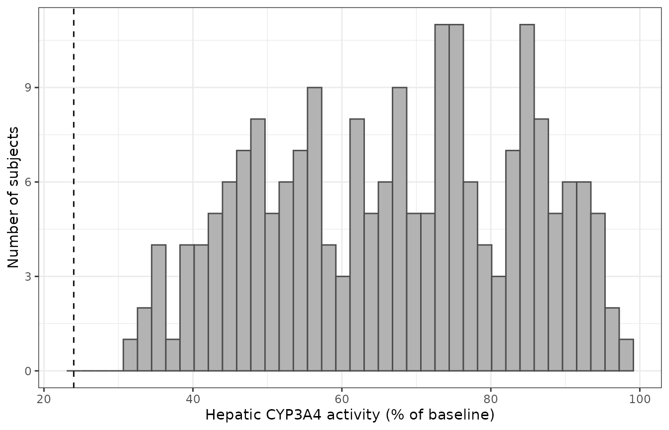
Distribution of steady-state hepatic CYP3A4 activity across 200 virtual rheumatoid-arthritis subjects whose IL-6 levels are drawn from the paper’s Figure 1b lognormal. The dashed line is the Emin floor of 24%.
The cohort median is 68% of baseline activity, matching the median
IL-6 of 54 pg/mL, and the 5th percentile approaches but never crosses
the 24% floor that Emin imposes.
Assumptions and deviations
Recorded because the paper does not state them, or because this implementation deliberately departs from the published analysis.
-
The victim-drug layer is not implemented.
Simvastatin and cyclosporine exposure predictions (case studies 1, 2 and
3, Figures 2, 3 and 5) require Simcyp V11.0 population-library values –
microsomal protein per gram of liver, liver weight, CYP3A4 abundance,
hepatic blood flow, and the
Qgutabsorption model – none of which was available. Supplementary Tables S1 and S2 give the compound layers but not the scalars needed to use them. No substitute was taken from a textbook or from another paper. -
Enzyme baseline
E0is carried as 1. The paper definesE0as the basal amount of hepatic CYP3A but never prints a value, and reports every outcome as a percentage of baseline.E0cancels exactly out of Eq. 1 under this normalisation, so no information is lost. The siblingChen_2024_interleukin6_cyp3a_pbpkuses the absolute-abundance normalisation instead, because that paper does print abundances. -
No intestinal CYP3A4 state. The paper assumed gut
suppression equalled the hepatic magnitude, but implemented it by
lowering intestinal abundance directly in the Simcyp population library
rather than with a second turnover equation, and never reported an
intestinal
kdeg. Adding a gut pool would require inventing that constant. (Chen_2024does carry a gut pool, with akdegof 0.03/h that its source publishes.) -
No between-subject variability and no residual
error. The paper reports no variance, %CV or confidence
interval for
CL,Vss,Emin,EC50orkdeg; the two IL-6 disposition parameters are single fitted point estimates and the three enzyme constants are single fixed inputs. Simcyp would have applied population-library variability, but none is printed, so noetais declared andpropSdisfixed(0)rather than invented. The cohort above therefore derives its spread from the paper’s published IL-6 population distributions, which is the only variability the source quantifies. -
The IL-6 disposition parameters are apparent, not
physiological.
Vss0.43 L/kg withCL1.0 L/h implies a roughly 21 h half-life at 70 kg, far longer than the minutes-to-hours half-life of exogenous IL-6. They were fitted to the slow rise and decline of disease IL-6 profiles in which endogenous synthesis is ongoing, so they describe the observed profile shape rather than IL-6 turnover. Users driving this model with a genuine exogenous IL-6 dose should be aware of that. -
R1andTfor case study 3 are not published. The perturbation arms in Check 5 back-solveR1from the published observed peak range (440-1228 pg/mL) at an assumedTof 7 days. The peaks are source values;R1andTare illustrative. The check that matters there is the exact agreement between the ODE solve and Supplementary Eq. 1 / Eq. 2, which does not depend on either. -
Body weight is fixed at 70 kg.
Vssis reported in L/kg, so weight scales the volume linearly, but no weight distribution is reported for any case study (Simcyp generated them internally). Weight does not affect any steady-state result, sinceCss = R/CLis volume-independent. -
The postsurgical geometric mean is 3.3% low.
exp(5.4)= 221 pg/mL against a reported 229. The paper rounds thatmuto two significant figures; 5.434 would reproduce 229 exactly. Excluded from the gate as a reporting-precision artefact. - Case study 4’s Figure 6 has no value table. The comparison there is against the reported inverse trend and “good agreement” claim, not against digits. The four clamp predictions are tabulated above so a reader can check them against the figure.
Session info
sessionInfo()
#> R version 4.6.1 (2026-06-24)
#> Platform: x86_64-pc-linux-gnu
#> Running under: Ubuntu 24.04.5 LTS
#>
#> Matrix products: default
#> BLAS:   /usr/lib/x86_64-linux-gnu/openblas-pthread/libblas.so.3
#> LAPACK: /usr/lib/x86_64-linux-gnu/openblas-pthread/libopenblasp-r0.3.26.so;  LAPACK version 3.12.0
#>
#> locale:
#>  [1] LC_CTYPE=C.UTF-8       LC_NUMERIC=C           LC_TIME=C.UTF-8
#>  [4] LC_COLLATE=C.UTF-8     LC_MONETARY=C.UTF-8    LC_MESSAGES=C.UTF-8
#>  [7] LC_PAPER=C.UTF-8       LC_NAME=C              LC_ADDRESS=C
#> [10] LC_TELEPHONE=C         LC_MEASUREMENT=C.UTF-8 LC_IDENTIFICATION=C
#>
#> time zone: UTC
#> tzcode source: system (glibc)
#>
#> attached base packages:
#> [1] stats     graphics  grDevices utils     datasets  methods   base
#>
#> other attached packages:
#> [1] ggplot2_4.0.3         dplyr_1.2.1           PKNCA_0.12.1
#> [4] rxode2_5.1.8          nlmixr2lib_0.3.2.9000
#>
#> loaded via a namespace (and not attached):
#>  [1] gtable_0.3.6        xfun_0.61           bslib_0.12.0
#>  [4] rxode2lincmt_0.1.0  lattice_0.22-9      vctrs_0.7.3
#>  [7] tools_4.6.1         generics_0.1.4      parallel_4.6.1
#> [10] tibble_3.3.1        symengine_0.2.14    pkgconfig_2.0.3
#> [13] data.table_1.18.6.1 checkmate_2.3.4     RColorBrewer_1.1-3
#> [16] S7_0.2.2            desc_1.4.3          lifecycle_1.0.5
#> [19] compiler_4.6.1      farver_2.1.2        textshaping_1.0.5
#> [22] fontawesome_0.5.3   htmltools_0.5.9     sys_3.4.3
#> [25] sass_0.4.10         yaml_2.3.12         tidyr_1.3.2
#> [28] pillar_1.11.1       pkgdown_2.2.1       crayon_1.5.3
#> [31] jquerylib_0.1.4     whisker_0.4.1       openssl_2.4.2
#> [34] cachem_1.1.0        nlme_3.1-169        tidyselect_1.2.1
#> [37] digest_0.6.39       lotri_1.0.5         purrr_1.2.2
#> [40] labeling_0.4.3      rxode2ll_2.0.18     fastmap_1.2.0
#> [43] grid_4.6.1          cli_3.6.6           dparser_1.3.1-14
#> [46] magrittr_2.0.5      withr_3.0.3         scales_1.4.0
#> [49] backports_1.5.1     rmarkdown_2.32      otel_0.2.0
#> [52] askpass_1.2.1       ragg_1.5.2          memoise_2.0.1
#> [55] evaluate_1.0.5      knitr_1.52          rex_1.2.2
#> [58] PreciseSums_0.7     rlang_1.3.0         downlit_0.4.5
#> [61] Rcpp_1.1.2          glue_1.8.1          xml2_1.6.0
#> [64] jsonlite_2.0.0      R6_2.6.1            systemfonts_1.3.2
#> [67] fs_2.1.0