Pulmonary TB treatment-outcome multistate model (Lin 2024) • nlmixr2lib

Model and source

Citation: Lin YJ, Zou Y, Karlsson MO, Svensson EM. A pharmacometric multistate model for predicting long-term treatment outcomes of patients with pulmonary TB. J Antimicrob Chemother. 2024;79(10):2561-2569. doi:10.1093/jac/dkae256. PMCID: PMC11441995. Open Access under CC BY. Structural equations from Supplementary Data ‘Model equations’ (equations 1-9) and the verbatim NONMEM control stream in Supplementary Data ‘NONMEM code’ (pages 12-16); parameter values from Supplementary Table S2 cross-checked against the control stream $THETA block. The two model-derived covariates are secondary metrics of Svensson EM, Karlsson MO. J Antimicrob Chemother. 2017;72(12):3398-3405; see modellib(‘Svensson_2017_bedaquiline’).
Article: https://doi.org/10.1093/jac/dkae256
PMC record (open access): https://www.ncbi.nlm.nih.gov/pmc/articles/PMC11441995/
Supplementary data (model equations, Tables S1-S4, and the full NONMEM control stream): https://doi.org/10.1093/jac/dkae256, “Supplementary data” at JAC Online

This is a pharmacometric multistate model, not a pharmacokinetic model. It carries no drug in any compartment: the five ODE states hold the marginal state-occupancy probability of a patient being in each of five clinical states at time t, and the ODEs are the Kolmogorov forward equations of a continuous-time Markov process whose transition intensities are the estimated hazards. Bedaquiline exposure never enters the model directly; it reaches the model through two model-derived covariates that are secondary metrics of the upstream mycobacterial-load model modellib("Svensson_2017_bedaquiline").

Because there is no drug concentration and no dosing event, the usual PKNCA validation does not apply. This vignette validates the model the way the source paper does: by checking that its state-occupancy predictions reproduce the published hazard shapes, hazard ratios, scenario percentages and 120-week population proportions, and that the probability mass is conserved.

Model structure

The five states and the transitions between them (Lin 2024 Figure 1):

State	Name	Definition (Lin 2024 Methods)
`s_activeTb`	Active TB	Active tuberculosis after initial infection; all patients start here
`s_converted`	Converted	Day of the first of two negative sputum cultures at least 25 days apart, not interrupted by a positive culture
`s_recurrentTb`	Recurrent TB	Day of the first of two consecutive positive cultures (or a single positive before study completion) after conversion
`s_dropout`	Dropout	Discontinued study visits for any reason except death; absorbing
`s_death`	Death	Death from any state; absorbing

Transitions: 1 -> 2 (conversion), 2 -> 3 (recurrence), 3 -> 2 (re-conversion), 1 -> 4, 2 -> 4, 3 -> 4 (dropout), and 1 -> 5, 2 -> 5, 3 -> 5 (death). Active TB is never re-entered.

Population

The model was developed on 402 patients pooled from two Janssen phase IIb bedaquiline trials: TMC207-C208 (NCT00449644, randomized, double-blind, placebo-controlled, newly diagnosed MDR-TB, n = 195) and TMC207-C209 (NCT00910871, open-label, single-arm, MDR-TB and XDR-TB including treatment-experienced patients, n = 207). Of 439 enrolled patients, 35 with negative cultures at both screening and baseline and 2 with only pre-treatment observations were excluded.

Baseline characteristics (Lin 2024 Table 1): median age 33 years (18-68), median weight 55 kg (30-113), 35% female, median baseline MGIT time-to-positivity 9.1 days (2.3-42). Drug-resistance profile: 3% drug-sensitive, 54% MDR, 28% pre-XDR, 14% XDR (pre-2021 WHO definitions); ~16% had a missing profile and were assigned to the MDR group. Comorbidity and severity: 96% had lung cavitation, 9% were living with HIV, 46% had prior anti-TB treatment, 75% came from a high-TB-burden country. Bedaquiline was given to 75% of patients (400 mg once daily for 2 weeks, then 200 mg three times weekly for 22 more weeks) on top of a multidrug background regimen; the remainder received placebo plus background regimen. Follow-up ran to 120 weeks: a 24-week investigational treatment period plus a 96-week follow-up period.

The dataset holds 6984 state observations with 364 conversion events (25 of them a second conversion after a recurrence), 63 recurrences, 114 dropouts and 30 deaths (Lin 2024 Figure 1).

The same information is available programmatically via readModelDb("Lin_2024_TB_multistate")()$population.

Source trace

Every ini() entry in inst/modeldb/therapeuticArea/Lin_2024_TB_multistate.R carries an in-file comment naming its source. The table below collects them.

Two conventions are worth stating up front, because they explain every apparent mismatch between this file and the published table:

Rates vs. mean transit times. Supplementary Table S2 reports the constant hazards as rates in week^-1. The NONMEM control stream parameterises the same quantities as mean transit times (MTT) in weeks, converted to hours (THETA(n)*24*7) because the estimation dataset runs on an hour axis. This model file uses Table S2’s week^-1 rate form, so each structural value below is the reciprocal of the corresponding $THETA. Worked example: THETA(1) = 295.375 weeks, so lambda23 = 1/295.375 = 0.00338554 week^-1, which rounds to the 0.00339 printed in Table S2.
Unrounded values. Where the control stream $THETA block carries more digits than Table S2, the unrounded value is used. The two agree on every parameter after rounding, which is itself a useful check that the printed control stream is the final run and not an earlier one.

Equation / parameter	Value in this model	Source location
Multistate ODE system (5 states)	n/a	Supplement “Model equations”, equations 1-5; control stream `$DES` `DADT(1)`-`DADT(5)`
Surge hazard form for `lambda12`	`SA/(((t-PT)/SW)^2+1)`	Supplement equation 8; control stream `$DES` `HZ12`
Weibull hazard form for `lambda15`/`lambda35`	`scaleshape(scale*t)^(shape-1)`	Supplement equation 7; control stream `$DES` `WB15`
Proportional-hazard covariate form	`lambda_ij,p = lambda_ij * exp(beta*(X_p - X_median))`	Supplement equation 9
`lsa12`	`log(0.18967032)`	Table S2 `SA12` = 0.190 /week (RSE 9.5%); `$THETA 7`/10000*168
`lpt12`	`log(11.3799)`	Table S2 `PT12` = 11.4 week (RSE 6.4%); `$THETA 8`
`lsw12`	`log(5.58883)`	Table S2 `SW12` = 5.59 week (RSE 12%); `$THETA 9`
`llambda23`	`log(1/295.375)`	Table S2 `lambda23` = 0.00339 /week (RSE 14%); `$THETA 1` (MTT23)
`llambda32`	`log(1/61.8711)`	Table S2 `lambda32` = 0.0162 /week (RSE 21%); `$THETA 2` (MTT32)
`llambda14`	`log(1/260.086)`	Table S2 `lambda14` = 0.00384 /week (RSE 21%); `$THETA 3` (MTT14)
`llambda24`	`log(1/667.209)`	Table S2 `lambda24/34` = 0.00150 /week (RSE 18%); `$THETA 4` (MTT24); `MTT34 = MTT24`
`llambda25`	`log(1/3803.44)`	Table S2 `lambda25` = 0.000263 /week (RSE 38%); `$THETA 6` (MTT25)
`lscale15`	`log(1/192.364)`	Table S2 `Scale15/35` = 0.00520 /week (RSE 18%); `$THETA 5` (MTT15); `MTT35 = MTT15`
`lshape15`	`log(1.96131)`	Table S2 `Shape15/35` = 1.96 (RSE 19%); `$THETA 10`
`e_hl2_sa12pt12`	`-0.686145`	Table S2 `betaHL2 on SA12, PT12` = -0.686 (RSE 16%); `$THETA 12`
`e_ttp_pt12sw12`	`0.442668`	Table S2 `betabasTTP on PT12, SW12` = 0.443 (RSE 20%); `$THETA 11`
`e_xdr_sa12`	`-0.622792`	Table S2 `betaXDR-TB on SA12` = -0.623 (RSE 29%); `$THETA 13`
`e_sexf_lambda23`	`-0.812999`	Table S2 `betasex on lambda23` = -0.813 (RSE 41%); `$THETA 17`
`e_mblend_lambda23`	`0.0371081`	Table S2 `betaMMBLend on lambda23` = 0.0371 (RSE 41%); `$THETA 18`
`e_study_lambda1424`	`0.909188`	Table S2 `betastudy on lambda14/24/34` = 0.910 (RSE 22%); `$THETA 14`
`e_age_lambda1424`	`-0.0230092`	Table S2 `betaage on lambda14/24/34` = -0.0230 (RSE 38%); `$THETA 15`
`e_baswt_lambda1525`	`-0.0838138`	Table S2 `betabasWT on lambda15/25/35` = -0.0838 (RSE 26%); `$THETA 16`
`MBL_HL_WK2` centering 0.69443 week	n/a	Control stream `$PK`; Lin 2024 Figure 3 reference individual
`TTP_MGIT_BASE` centering 9.06944 day	n/a	Control stream `$PK` (217.6667 h / 24); Lin 2024 Table 1 median 9.1 days
`MBL_END` centering 5.5726e-05	n/a	Control stream `$DES` `LOG(0.000055726)`; Figure 3 reference `-4.3 log10`
`AGE` centering 33 year	n/a	Control stream `$DES`; Lin 2024 Table 1 median
`WT` centering 55 kg	n/a	Control stream `$DES`; Lin 2024 Table 1 median
No IIV (no eta parameters)	n/a	Control stream `$OMEGA 0 FIX`; `BSV = ETA(1)` is an explicit “place holder”
`addSd` placeholder residual	`0.001`	Not from the source – see Assumptions and deviations

The reference individual

Lin 2024 Figure 3 defines a reference individual against which all covariate effects are expressed: a 33-year-old male weighing 55 kg, infected with MDR tuberculosis, enrolled in the C209 study, with 9.1 days of baseline time-to-positivity, 0.69 weeks of half-life of bacterial clearance at week 2, and -4.3 log10(MMBLend).

mod <- readModelDb("Lin_2024_TB_multistate")

reference_individual <- data.frame(
  AGE               = 33,        # years                (Figure 3: "33-year-old")
  WT                = 55,        # kg                   (Figure 3: "weighing 55 kg")
  SEXF              = 0,         # male                 (Figure 3: "male")
  STUDY_C208        = 0,         # C209                 (Figure 3: "enrolled in the C209 study")
  DIS_TB_XDR_STRICT = 0,         # MDR, not XDR         (Figure 3: "infected with MDR tuberculosis")
  TTP_MGIT_BASE     = 9.1,       # days                 (Figure 3: "9.1 days of baseline time-to-positivity")
  MBL_HL_WK2        = 0.69443,   # weeks                (Figure 3: "0.69 weeks of half-life")
  MBL_END           = 10^(-4.3)  # n bacteria/inoculum  (Figure 3: "-4.3 log10(MMBLend)")
)

knitr::kable(
  reference_individual |>
    tidyr::pivot_longer(everything(), names_to = "Covariate", values_to = "Value"),
  digits  = 5,
  caption = "Reference individual of Lin 2024 Figure 3."
)

Reference individual of Lin 2024 Figure 3.
Covariate	Value
AGE	33.00000
WT	55.00000
SEXF	0.00000
STUDY_C208	0.00000
DIS_TB_XDR_STRICT	0.00000
TTP_MGIT_BASE	9.10000
MBL_HL_WK2	0.69443
MBL_END	0.00005

Note that MBL_END is stored on the natural scale. The paper’s figures are labelled in log10(MMBLend) while the model coefficient is per unit of natural log, so 10^(-4.3) = 5.01e-05 here is the natural-scale value corresponding to the figure’s -4.3. It is within rounding of the control stream’s centering constant 5.5726e-05 (whose log10 is -4.2537).

# Weekly observation grid over the full 120-week study, on the s_converted ODE
# state. rxode2 returns every algebraic observable (prob_scc, prob_death, the
# individual hazards, ...) as a column at these rows.
obs_times <- seq(0, 120, by = 0.25)

make_events <- function(cov, id_offset = 0L) {
  cov |>
    dplyr::mutate(id = id_offset + dplyr::row_number()) |>
    tidyr::crossing(time = obs_times) |>
    dplyr::mutate(evid = 0L, amt = NA_real_, cmt = "s_converted") |>
    dplyr::arrange(id, time)
}

Replicate Figure 2 – the conversion surge hazard

Lin 2024 Figure 2 plots the conversion hazard lambda12 over the first 24 weeks, stratified by the half-life of bacterial clearance at week 2 (5th / 50th / 95th percentiles), baseline time-to-positivity (5th / 50th / 95th percentiles) and XDR status. Figure 6 gives the percentile values used: MBL_HL_WK2 0.33 / 0.69 / 1.1 weeks and TTP_MGIT_BASE 4.2 / 9.1 / 38 days.

fig2_grid <- tidyr::expand_grid(
  MBL_HL_WK2        = c(0.33, 0.69443, 1.1),
  TTP_MGIT_BASE     = c(4.2, 9.1, 38),
  DIS_TB_XDR_STRICT = c(0, 1)
) |>
  dplyr::mutate(
    AGE = 33, WT = 55, SEXF = 0, STUDY_C208 = 0, MBL_END = 10^(-4.3),
    hl_lab  = factor(MBL_HL_WK2,
                     labels = c("HL2 0.33 wk (5th)", "HL2 0.69 wk (50th)", "HL2 1.1 wk (95th)")),
    ttp_lab = factor(TTP_MGIT_BASE,
                     labels = c("TTP 4.2 d (5th)", "TTP 9.1 d (50th)", "TTP 38 d (95th)")),
    xdr_lab = ifelse(DIS_TB_XDR_STRICT == 1, "XDR", "non-XDR")
  )

fig2_sim <- rxode2::rxSolve(
  mod, events = make_events(fig2_grid),
  keep = c("hl_lab", "ttp_lab", "xdr_lab")
) |>
  as.data.frame()
#> Warning: multi-subject simulation without without 'omega'

fig2_sim |>
  dplyr::filter(time <= 24) |>
  ggplot(aes(time, lambda12, colour = hl_lab, linetype = xdr_lab)) +
  geom_line(linewidth = 0.7) +
  facet_wrap(~ttp_lab) +
  labs(
    x = "Time (weeks)", y = expression(lambda[12] ~ " (conversion hazard, 1/week)"),
    colour = NULL, linetype = NULL,
    title = "Figure 2 -- conversion surge hazard",
    caption = "Replicates Figure 2 of Lin 2024."
  ) +
  theme(legend.position = "bottom")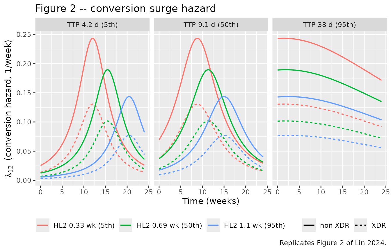

Two published quantities are checked exactly.

# 1. Peak time of the conversion hazard for the reference individual.
ref_sim  <- rxode2::rxSolve(mod, events = make_events(reference_individual)) |> as.data.frame()
peak_obs <- ref_sim$time[which.max(ref_sim$lambda12)]

# 2. XDR effect on the surge amplitude: the paper reports a 46% decrease.
xdr_hr <- exp(rxode2::rxode(mod)$theta[["e_xdr_sa12"]])

surge_checks <- tibble::tibble(
  Quantity  = c("Peak time of lambda12 (weeks)", "XDR-TB reduction in lambda12 (%)"),
  Simulated = c(peak_obs, 100 * (1 - xdr_hr)),
  Published = c(11.4, 46),
  `Published interval` = c("95% CI 10.0-12.8", "95% CI 24-62")
)

knitr::kable(surge_checks, digits = 2,
             caption = "Figure 2 / Results checks against Lin 2024.")

Figure 2 / Results checks against Lin 2024.
Quantity	Simulated	Published	Published interval
Peak time of lambda12 (weeks)	11.25	11.4	95% CI 10.0-12.8
XDR-TB reduction in lambda12 (%)	46.36	46.0	95% CI 24-62

The simulated peak sits marginally below the printed 11.4 weeks because the reference individual’s baseline TTP of 9.1 days is very slightly above the model’s centering constant of 9.06944 days, which shifts PT12 down by exp(-0.442668 * (9.1 - 9.06944)/7) = 0.998; the remaining difference is the 0.25-week resolution of the observation grid.

Replicate Figure 3 – predictor hazard ratios

Figure 3 is a forest plot of hazard ratios relative to the reference individual for recurrence, dropout and death. The hazard ratios are pure functions of the estimated coefficients, so they can be checked in closed form.

th <- rxode2::rxode(mod)$theta

hazard_ratios <- tibble::tribble(
  ~Transition,        ~Predictor,                          ~Contrast,                  ~`Hazard ratio`,
  "Recurrence",       "Sex",                               "female vs male",           exp(th[["e_sexf_lambda23"]]),
  "Recurrence",       "log10(MMBLend)",                    "+1 log10 unit",            exp(th[["e_mblend_lambda23"]] * log(10)),
  "Dropout (any)",    "Study",                             "C208 vs C209",             exp(th[["e_study_lambda1424"]]),
  "Dropout (any)",    "Age",                               "-10 years (23 vs 33)",     exp(th[["e_age_lambda1424"]] * -10),
  "Death (any)",      "Baseline weight",                   "-10 kg (45 vs 55)",        exp(th[["e_baswt_lambda1525"]] * -10),
  "Conversion (SA12)","XDR-TB",                            "XDR vs non-XDR",           exp(th[["e_xdr_sa12"]])
)

knitr::kable(hazard_ratios, digits = 3,
             caption = paste("Figure 3 -- hazard ratios relative to the reference individual.",
                             "Directions match Lin 2024 Results: men and higher end-of-treatment",
                             "mycobacterial load raise recurrence; C208 enrollment and younger age",
                             "raise dropout; lower baseline weight raises death."))

Figure 3 – hazard ratios relative to the reference individual. Directions match Lin 2024 Results: men and higher end-of-treatment mycobacterial load raise recurrence; C208 enrollment and younger age raise dropout; lower baseline weight raises death.
Transition	Predictor	Contrast	Hazard ratio
Recurrence	Sex	female vs male	0.444
Recurrence	log10(MMBLend)	+1 log10 unit	1.089
Dropout (any)	Study	C208 vs C209	2.482
Dropout (any)	Age	-10 years (23 vs 33)	1.259
Death (any)	Baseline weight	-10 kg (45 vs 55)	2.312
Conversion (SA12)	XDR-TB	XDR vs non-XDR	0.536

Each direction reproduces a statement in Lin 2024 Results and Discussion: women have 0.444 times the recurrence hazard of men (“the risk of recurrence was higher for men”); C208 patients have 2.48 times the dropout hazard of C209 patients (“The dropout rate in patients from the C208 study was higher than in C209”); a 10 kg lower baseline weight raises the death hazard 2.31-fold (“lower weight at baseline was correlated with a higher risk of death”).

Replicate Figure 6 – scenario simulations

Figure 6 is the paper’s most sharply specified prediction, and therefore the strongest available falsification test: it names the exact covariate values of each scenario and reports the resulting percentage of patients who had reached sputum culture conversion at 24 weeks. Every covariate other than half-life and time-to-positivity is set to the reference individual’s value.

Because the model has no between-subject variability, each scenario is a single deterministic trajectory, so the published median percentages are directly reproducible without simulating a cohort.

scenarios <- tidyr::expand_grid(
  MBL_HL_WK2    = c(`high clearance` = 0.33, `low clearance` = 1.1),
  TTP_MGIT_BASE = c(`high burden` = 4.2, `low burden` = 38)
) |>
  dplyr::mutate(
    AGE = 33, WT = 55, SEXF = 0, STUDY_C208 = 0,
    DIS_TB_XDR_STRICT = 0, MBL_END = 10^(-4.3),
    scenario = paste0(
      ifelse(MBL_HL_WK2 == 0.33, "High clearance", "Low clearance"), ", ",
      ifelse(TTP_MGIT_BASE == 4.2, "high burden", "low burden")
    )
  )

scen_sim <- rxode2::rxSolve(mod, events = make_events(scenarios), keep = "scenario") |>
  as.data.frame()
#> Warning: multi-subject simulation without without 'omega'

scen_sim |>
  dplyr::select(time, scenario, `Active TB` = prob_active_tb, Converted = prob_scc,
                `Recurrent TB` = prob_recurrent_tb, Dropout = prob_dropout, Death = prob_death) |>
  tidyr::pivot_longer(-c(time, scenario), names_to = "State", values_to = "Probability") |>
  ggplot(aes(time, Probability, colour = State)) +
  geom_line(linewidth = 0.7) +
  geom_vline(xintercept = 24, linetype = "dotted") +
  facet_wrap(~scenario) +
  labs(x = "Time (weeks)", y = "Proportion of patients",
       title = "Figure 6 -- predicted outcomes by disease-severity scenario",
       caption = paste("Replicates Figure 6 of Lin 2024. Dotted line marks the end of the",
                       "24-week investigational treatment period.")) +
  theme(legend.position = "bottom")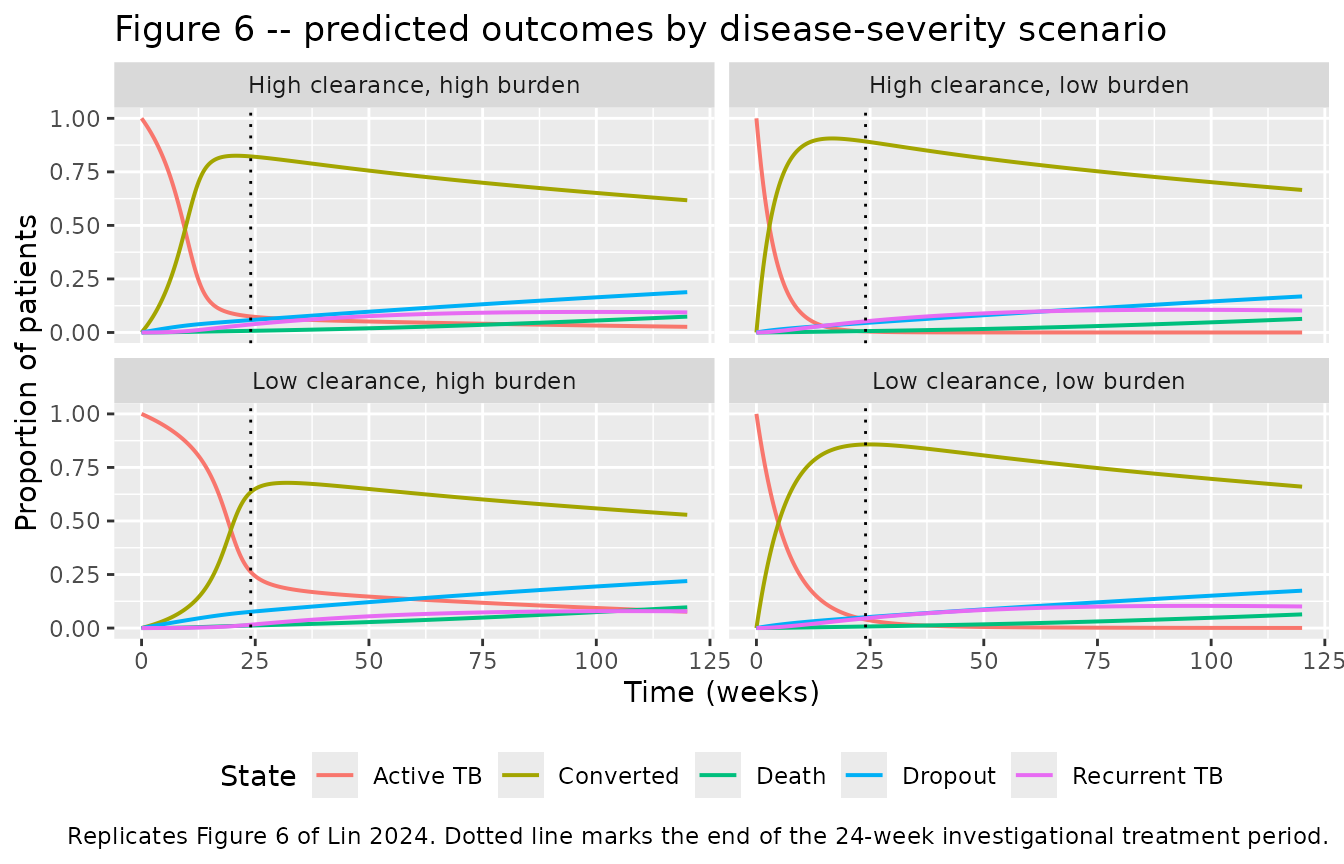

scc_24 <- scen_sim |>
  dplyr::filter(time == 24) |>
  dplyr::transmute(scenario, `SCC at 24 weeks (%)` = 100 * prob_scc)

scc_compare <- scc_24 |>
  dplyr::mutate(
    Published = dplyr::case_when(
      scenario == "Low clearance, high burden"  ~ 62,   # "the most severe scenario"
      scenario == "High clearance, low burden"  ~ 89,   # "the least severe scenario"
      TRUE                                      ~ NA_real_
    ),
    `Published interval` = dplyr::case_when(
      scenario == "Low clearance, high burden"  ~ "90% PI 51-69",
      scenario == "High clearance, low burden"  ~ "90% PI 86-90",
      TRUE                                      ~ NA_character_
    ),
    `Difference (pp)` = `SCC at 24 weeks (%)` - Published
  ) |>
  dplyr::rename("Scenario" = scenario, "Published (%)" = Published)

knitr::kable(scc_compare, digits = 1,
             caption = paste("Sputum culture conversion at 24 weeks, simulated vs. Lin 2024",
                             "Results: 'the proportions of patients who reached SCC ranged from",
                             "62% (90% PI, 51%-69%) (the most severe scenario) to 89% (90% PI,",
                             "86%-90%) (the least severe scenario)'. Only the two extreme",
                             "scenarios carry published point estimates."))

Sputum culture conversion at 24 weeks, simulated vs. Lin 2024 Results: ‘the proportions of patients who reached SCC ranged from 62% (90% PI, 51%-69%) (the most severe scenario) to 89% (90% PI, 86%-90%) (the least severe scenario)’. Only the two extreme scenarios carry published point estimates.
Scenario	SCC at 24 weeks (%)	Published (%)	Published interval	Difference (pp)
High clearance, high burden	82.2	NA	NA	NA
High clearance, low burden	89.2	89	90% PI 86-90	0.2
Low clearance, high burden	63.5	62	90% PI 51-69	1.5
Low clearance, low burden	85.7	NA	NA	NA

Both published extremes are reproduced to within about one percentage point, and the two intermediate scenarios fall between them, as Figure 6 shows. The paper’s qualitative conclusion also reproduces: recurrence rises substantially after 24 weeks in the low-clearance scenarios irrespective of baseline bacterial burden, whereas conversion at 24 weeks depends on both.

Replicate Figure 4 – population predictions over 120 weeks

Figure 4 is a visual predictive check of the proportion of patients in each state over the full study. Reproducing it needs a cohort whose covariate distribution approximates Table 1. Lin 2024 publishes medians and ranges but not the joint covariate distribution, so the cohort below is an approximation – see Assumptions and deviations.

set.seed(20240701)
n_cohort <- 200  # per the 200-per-arm cap; this is a single-arm cohort

# Log-normal SD implied by a median and a published 95th percentile.
sd_from_p95 <- function(median, p95) (log(p95) - log(median)) / qnorm(0.95)

cohort <- data.frame(
  AGE               = pmin(pmax(round(rlnorm(n_cohort, log(33), 0.28)), 18), 68),
  WT                = pmin(pmax(round(rlnorm(n_cohort, log(55), 0.21)), 30), 113),
  SEXF              = rbinom(n_cohort, 1, 0.35),
  STUDY_C208        = rbinom(n_cohort, 1, 0.485),
  DIS_TB_XDR_STRICT = rbinom(n_cohort, 1, 0.12),
  TTP_MGIT_BASE     = pmin(pmax(rlnorm(n_cohort, log(9.1), sd_from_p95(9.1, 38)), 2.3), 42),
  MBL_HL_WK2        = rlnorm(n_cohort, log(0.69443), sd_from_p95(0.69443, 1.1)),
  MBL_END           = rlnorm(n_cohort, log(5.5726e-05), 1.8)
)

cohort_events <- make_events(cohort)
stopifnot(!anyDuplicated(unique(cohort_events[, c("id", "time", "evid")])))

cohort_sim <- rxode2::rxSolve(mod, events = cohort_events) |> as.data.frame()
#> Warning: multi-subject simulation without without 'omega'

# rxSolve silently drops subjects on some failure modes -- assert the count.
stopifnot(dplyr::n_distinct(cohort_sim$id) == n_cohort)

state_labels <- c(prob_active_tb = "Active TB", prob_scc = "Converted",
                  prob_recurrent_tb = "Recurrent TB", prob_dropout = "Dropout",
                  prob_death = "Death")

cohort_long <- cohort_sim |>
  dplyr::select(id, time, dplyr::all_of(names(state_labels))) |>
  tidyr::pivot_longer(-c(id, time), names_to = "state", values_to = "p") |>
  dplyr::mutate(State = factor(state_labels[state], levels = unname(state_labels)))

cohort_long |>
  dplyr::group_by(time, State) |>
  dplyr::summarise(Mean = mean(p), .groups = "drop") |>
  ggplot(aes(time, Mean, colour = State)) +
  geom_line(linewidth = 0.8) +
  geom_vline(xintercept = 24, linetype = "dotted") +
  labs(x = "Time (weeks)", y = "Proportion of patients",
       title = "Figure 4 -- predicted proportion of patients in each state",
       caption = paste("Replicates Figure 4 of Lin 2024 (model-predicted proportions only;",
                       "the observed proportions are not publicly available).")) +
  theme(legend.position = "bottom")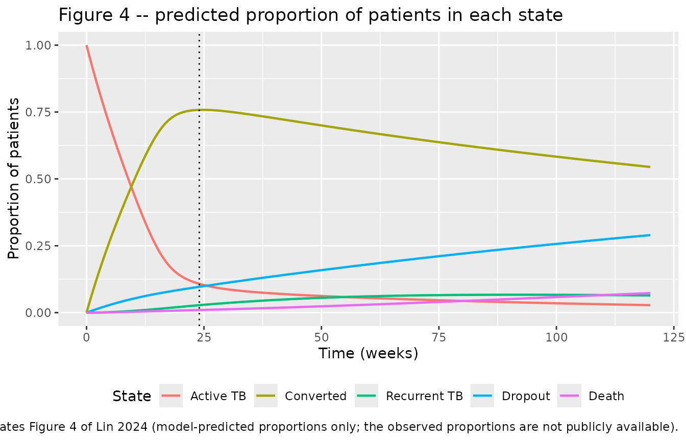

at_120 <- cohort_sim |> dplyr::filter(time == 120)

pop_compare <- tibble::tibble(
  State       = c("Converted", "Recurrent TB", "Death", "Dropout"),
  `Simulated (%)` = 100 * c(mean(at_120$prob_scc), mean(at_120$prob_recurrent_tb),
                            mean(at_120$prob_death), mean(at_120$prob_dropout)),
  `Published (%)` = c(55, 6.5, 7.5, 28.4),
  `Published interval` = c("95% PI 50-60", "95% PI 4.2-9.0", "95% PI 5.2-10",
                           "observed 114/402")
) |>
  dplyr::mutate(`Difference (pp)` = `Simulated (%)` - `Published (%)`)

knitr::kable(pop_compare, digits = 1,
             caption = paste("Predicted proportion of patients in each state at 120 weeks.",
                             "Converted, recurrent TB and death are the model-predicted values",
                             "with prediction intervals from Lin 2024 Results; the dropout row",
                             "is the observed 114 of 402 patients from Lin 2024 Figure 1."))

Predicted proportion of patients in each state at 120 weeks. Converted, recurrent TB and death are the model-predicted values with prediction intervals from Lin 2024 Results; the dropout row is the observed 114 of 402 patients from Lin 2024 Figure 1.
State	Simulated (%)	Published (%)	Published interval	Difference (pp)
Converted	54.5	55.0	95% PI 50-60	-0.5
Recurrent TB	6.4	6.5	95% PI 4.2-9.0	-0.1
Death	7.3	7.5	95% PI 5.2-10	-0.2
Dropout	29.0	28.4	observed 114/402	0.6

All three published model predictions and the observed dropout proportion are reproduced within about one percentage point.

Structural checks

PKNCA is not applicable to this model (no concentration, no dose). The checks below are the multistate analogues: conservation of probability mass, correct absorbing behaviour, and the sign and shape of each hazard.

# 1. Mass balance. The five state-occupancy probabilities are a partition of
#    a probability space and must sum to exactly 1 at every time, for every
#    subject. This is the single strongest structural check available.
max_mass_error <- max(abs(cohort_sim$prob_state_sum - 1))

# 2. Every probability must stay within [0, 1].
probs <- cohort_sim[, names(state_labels)]
in_unit_interval <- all(probs >= -1e-10 & probs <= 1 + 1e-10)

# 3. Absorbing states must be monotone non-decreasing; the transient states
#    need not be (a patient can leave and re-enter the converted state).
monotone <- cohort_sim |>
  dplyr::arrange(id, time) |>
  dplyr::group_by(id) |>
  dplyr::summarise(
    dropout_monotone = all(diff(prob_dropout) >= -1e-10),
    death_monotone   = all(diff(prob_death)   >= -1e-10),
    active_monotone  = all(diff(prob_active_tb) <=  1e-10),  # never re-entered
    .groups = "drop"
  )

# 4. Initial conditions: everyone starts in active TB.
t0 <- cohort_sim |> dplyr::filter(time == 0)

structural <- tibble::tibble(
  Check = c(
    "max |sum of the 5 state probabilities - 1| over all subjects and times",
    "all state probabilities within [0, 1]",
    "s_dropout monotone non-decreasing in every subject",
    "s_death monotone non-decreasing in every subject",
    "s_activeTb monotone non-increasing in every subject (never re-entered)",
    "prob_active_tb == 1 at t = 0 in every subject",
    "all other state probabilities == 0 at t = 0"
  ),
  Result = c(
    format(max_mass_error, digits = 3),
    in_unit_interval,
    all(monotone$dropout_monotone),
    all(monotone$death_monotone),
    all(monotone$active_monotone),
    isTRUE(all.equal(t0$prob_active_tb, rep(1, nrow(t0)))),
    isTRUE(all.equal(sum(t0$prob_scc, t0$prob_recurrent_tb, t0$prob_dropout, t0$prob_death), 0))
  ) |> as.character()
)

knitr::kable(structural, caption = "Structural checks on the multistate ODE system.")

Structural checks on the multistate ODE system.
Check	Result
max \|sum of the 5 state probabilities - 1\| over all subjects and times	3.77e-15
all state probabilities within [0, 1]	TRUE
s_dropout monotone non-decreasing in every subject	TRUE
s_death monotone non-decreasing in every subject	TRUE
s_activeTb monotone non-increasing in every subject (never re-entered)	TRUE
prob_active_tb == 1 at t = 0 in every subject	TRUE
all other state probabilities == 0 at t = 0	TRUE

stopifnot(max_mass_error < 1e-8, in_unit_interval,
          all(monotone$dropout_monotone), all(monotone$death_monotone))

# The Weibull death hazard has shape 1.96 > 1, so it must increase over time;
# the conversion surge must rise to a single interior peak and fall away.
haz <- ref_sim |> dplyr::filter(time > 0)

hazard_shape <- tibble::tibble(
  Check = c(
    "lambda15 (Weibull, shape 1.96) strictly increasing over time",
    "lambda12 (surge) has a single interior maximum",
    "lambda12 at t = 0 is below its peak",
    "lambda23 steps up at week 26 when MBL_END is above its reference",
    "constant hazards lambda32, lambda14, lambda24, lambda25 are time-invariant"
  ),
  Result = as.character(c(
    all(diff(haz$lambda15) > 0),
    which.max(haz$lambda12) > 1 && which.max(haz$lambda12) < nrow(haz),
    haz$lambda12[1] < max(haz$lambda12),
    {
      hi <- reference_individual; hi$MBL_END <- 1e-3   # above the 5.57e-05 reference
      s  <- rxode2::rxSolve(mod, events = make_events(hi)) |> as.data.frame()
      before <- s$lambda23[which.min(abs(s$time - 25))]
      after  <- s$lambda23[which.min(abs(s$time - 27))]
      after > before
    },
    all(sapply(c("lambda32", "lambda14", "lambda24", "lambda25"),
               function(v) diff(range(haz[[v]])) < 1e-12))
  ))
)

knitr::kable(hazard_shape, caption = "Hazard-shape checks against the source's stated forms.")

Hazard-shape checks against the source’s stated forms.
Check	Result
lambda15 (Weibull, shape 1.96) strictly increasing over time	TRUE
lambda12 (surge) has a single interior maximum	TRUE
lambda12 at t = 0 is below its peak	TRUE
lambda23 steps up at week 26 when MBL_END is above its reference	TRUE
constant hazards lambda32, lambda14, lambda24, lambda25 are time-invariant	TRUE

Assumptions and deviations

Placeholder residual error. Lin 2024 fits the exact multistate event likelihood ($ESTIMATION METHOD=0 LIKE) on the observed categorical state and has no observation-error model ($SIGMA 0 FIX in the simulation variant of the control stream). This translation is intended for forward simulation, so a tiny additive residual (addSd = 0.001) is attached to prob_scc – the paper’s primary endpoint – purely so the nlmixr2 likelihood machinery accepts the model. This value is not from the source and should not be interpreted.
No between-subject variability. The control stream declares BSV = ETA(1) ; place holder and sets $OMEGA 0 FIX, so the fitted model carries no IIV. No eta parameters were invented, and every simulation in this vignette is deterministic given the covariates.
MMBLend time gate: 26 weeks, not 24. The main text says the end-of-treatment mycobacterial load acts on recurrence “after 24 weeks” and “after the completion of 24 week treatment”, but the control stream gates it at IF(WEEK.GT.26) FLAG_MMBL = 1. The control stream value (26 weeks) is used here, per the standing convention that a printed equation or control stream beats a prose gloss. The choice affects only a two-week window and, because the recurrence coefficient is small, moves the 120-week recurrence proportion by well under 0.1 percentage points.
XDR encoding is strict, not pooled. The control stream encodes XDR = 0; IF(TBTYPE.EQ.4) XDR = 1, which places the 95 pre-XDR patients (28% of the cohort) in the reference group. This model therefore uses the new DIS_TB_XDR_STRICT covariate rather than the existing DIS_TB_XDR, which pools pre-XDR with XDR for the Svensson 2017 bedaquiline model. The two are not interchangeable and substituting one for the other would misclassify more than a quarter of the cohort.
TTP_MGIT_BASE units and reference. The source data column MTTP is in hours, centered at 217.6667 h. This model uses the canonical TTP_MGIT_BASE column in days, so the identical arithmetic is written as (TTP_MGIT_BASE - 9.06944)/7; the divisor 7 reproduces the control stream’s /24/7, making the coefficient per week of baseline TTP. The 9.06944-day centering value is this cohort’s median and differs from the 6.8 days recorded for the Svensson 2017 C208-only cohort in the covariate register.
MBL_END scale. Stored on the natural scale and log-transformed inside model(). The coefficient is per unit of natural log, so the per-log10-unit hazard ratio is exp(0.0371081 * ln(10)) = 1.089. MBL_END must be strictly positive: log(0) is undefined and would propagate NaN through the whole solve even before the week-26 gate opens.
Virtual cohort distributions are approximate. Lin 2024 Table 1 publishes medians and ranges but not the joint covariate distribution, and reports no correlation structure. The cohort here draws age, weight, baseline TTP and week-2 half-life as independent log-normals calibrated to the published median and (where available) the 95th percentile from Figure 6, truncated to the published ranges; binary covariates are independent Bernoulli draws at the Table 1 marginal frequencies. MBL_END has no published dispersion at all, so its log-scale SD of 1.8 is a plausible-but-unverified choice; because the recurrence coefficient is small, the 120-week proportions are insensitive to it. Real covariates are correlated (XDR status, baseline TTP and bacterial clearance in particular), so the cohort understates the true spread. The scenario checks against Figure 6 do not depend on any of these assumptions, because the paper specifies those covariate values exactly.
Placebo and bedaquiline arms are not distinguished. Bedaquiline treatment was screened as a covariate and not retained on any transition; its effect reaches the model only through MBL_HL_WK2 and MBL_END. A user who wants an exposure-driven simulation should generate those two covariates from modellib("Svensson_2017_bedaquiline") rather than looking for a treatment flag here.
Screened but unused covariates. HIV status, lung cavitation, prior anti-TB treatment, bedaquiline treatment and time-varying albumin were all evaluated by Lin 2024 and not retained. They are recorded in the model file’s covariatesDataExcluded metadata for provenance rather than in covariateData, so they do not appear in model().
Observed data are not reproduced. Lin 2024 Figure 4 overlays observed state proportions on the predicted intervals. The individual patient data from TMC207-C208 and TMC207-C209 are not publicly available, so only the predicted proportions are shown here.