Inter-antibody variability in mAb PK (Kumar 2024)
Source:vignettes/articles/Kumar_2024_mAb_popPBPK.Rmd
Kumar_2024_mAb_popPBPK.RmdModel and source
- Citation: Kumar M, Lanke S, Yadav A, Ette M, Mager DE, Shah DK. Inter-Antibody Variability in the Clinical Pharmacokinetics of Monoclonal Antibodies Characterized Using Population Physiologically Based Pharmacokinetic Modeling. Antibodies. 2024;13(3):54. doi:10.3390/antib13030054
- Article: https://doi.org/10.3390/antib13030054
- Upstream framework: Shah DK, Betts AM. J Pharmacokinet Pharmacodyn. 2012;39(1):67-86. doi:10.1007/s10928-011-9232-2
Kumar 2024 takes the Shah & Betts 2012 platform PBPK model
(packaged separately as Shah_2012_mAb_PBPK) and turns it
into a population model in which the “individuals” are
antibodies rather than patients. Mean clinical plasma
profiles were digitised for 143 mAbs; 55 showed linear PK; 44 with IV
data built the IV model and the 16 that also had SC data built the SC
model. Two of the four Shah & Betts system parameters
(CLup, kdeg) were re-estimated with
inter-antibody random effects, and two new absorption parameters
(kSC, S_LU) were introduced for the SC
route.
Two model files come out of this one paper, matching the two models the authors built:
| File | Route | States | Estimated parameters |
|---|---|---|---|
Kumar_2024_mAb_popPBPK_iv |
IV | 93 |
CLup, kdeg (+ 2 etas) |
Kumar_2024_mAb_popPBPK_sc |
SC | 99 |
CLup, kdeg, kSC,
S_LU (+ 4 etas) |
mod_iv <- rxode2(readModelDb("Kumar_2024_mAb_popPBPK_iv"))
#> ℹ parameter labels from comments will be replaced by 'label()'
mod_sc <- rxode2(readModelDb("Kumar_2024_mAb_popPBPK_sc"))
#> ℹ parameter labels from comments will be replaced by 'label()'

c(iv_states = length(mod_iv$state), sc_states = length(mod_sc$state))
#> iv_states sc_states
#>        93        99
Population
The 44 IV antibodies and 16 SC antibodies are drawn overwhelmingly from published phase 1 single-dose and dose-escalation studies, in healthy volunteers and in patients (oncology, rheumatoid arthritis, asthma, psoriasis, infectious disease). Kumar 2024 Supplementary Table S3 lists per-antibody approval status, phase, country, and year.
Two deliberate exclusions define the model’s scope:
- Antibodies with dose-dependent (target-mediated) disposition were removed by dose-normalising the digitised profiles, so the model describes linear mAb disposition only and carries no TMDD terms.
- Panobacumab (an IgM) and suvratoxumab (Fc-modified) were dropped despite showing linear PK, because their FcRn affinity differs substantially from the rest of the IgG set.
The underlying human physiology is the Shah & Betts 2012 Table 4 71 kg male reference; there are no subject-level covariates in the model at all.
str(mod_iv$meta$population)
#> List of 11
#>  $ n_subjects    : num 44
#>  $ n_studies     : num 44
#>  $ age_range     : chr "adults (predominantly healthy-volunteer phase 1 cohorts)"
#>  $ weight_range  : chr "71 kg reference adult male (Shah and Betts 2012 Table 4 physiology)"
#>  $ sex_female_pct: num NA
#>  $ species       : chr "human"
#>  $ disease_state : chr "Mixed. Predominantly phase 1 single-dose studies in healthy volunteers, with some patient cohorts (oncology, rh"| __truncated__
#>  $ dose_range    : chr "multiple IV dose levels per antibody (digitized phase 1 dose-escalation profiles)"
#>  $ regions       : chr "multi-national (USA, Canada, Europe, Japan, Korea, China and others; Supplementary Table S3)"
#>  $ notes         : chr "The 'individuals' of this population model are ANTIBODIES, not human subjects. Mean (digitized) plasma concentr"| __truncated__
#>  $ scope_note    : chr "Simulating with the etas active generates a range of plausible ANTIBODY-level typical profiles (the paper's Mon"| __truncated__
Source trace
Every value in both ini() blocks, and each structural
choice, traced to its source location.
| Quantity | Value | Source |
|---|---|---|
CLup (pinocytosis per unit endosomal volume) |
0.32 L/h/L (RSE 5.6%) | Kumar 2024 Suppl. Table S2; abstract |
omega_CLup |
73% (RSE 3.2%) | Kumar 2024 Suppl. Table S2 |
kdeg (endosomal degradation, FcRn-unbound) |
26.1 1/h (RSE 11%) | Kumar 2024 Suppl. Table S2; abstract |
omega_kdeg |
46% (RSE 17.6%) | Kumar 2024 Suppl. Table S2 |
kSC (local degradation at injection site) |
0.0015 1/h (RSE 66%) | Kumar 2024 Suppl. Table S2; abstract |
omega_kSC |
193% (RSE 24.7%) | Kumar 2024 Suppl. Table S2 |
S_LU (lymphatic-uptake scaling) |
0.54 (RSE 14%) | Kumar 2024 Suppl. Table S2; abstract |
omega_S_LU |
49% (RSE 21.1%) | Kumar 2024 Suppl. Table S2 |
| Central plasma volume | 1412 mL | Kumar 2024 Section 2.5 |
| Central blood-cell volume | 1155 mL | Kumar 2024 Section 2.5 |
| Skin sub-volumes and flows (SC model) | Table 1 col. “Skin (SC)” | Kumar 2024 Table 1 |
| Subcutaneous sub-volumes and flows | Table 1 col. “SC (SC)” | Kumar 2024 Table 1 |
| All other organ volumes and flows (human, 71 kg) | Table 4 | Shah & Betts 2012 Table 4 |
Vascular reflection coefficients sigma_V
|
0.95 / 0.90 / 0.85, brain 0.99 | Shah & Betts 2012 “Model parameters” |
Lymphatic reflection coefficient sigma_IS
|
0.2 (all tissues) | Shah & Betts 2012 “Model parameters” |
| Lymph flow | plasma flow / 500 | Shah & Betts 2012 “Model parameters” |
| Endosomal FcRn concentration | 4.98e-5 M | Shah & Betts 2012 Table 6 |
FR (recycled fraction) |
0.715 | Shah & Betts 2012 “Model parameters” |
kon / koff (human) |
5.59e8 1/M/h, 23.9 1/h | Shah & Betts 2012 “Model parameters” |
| Lymph-node return flow | 3.670 L/h | Shah & Betts 2012 Table 4 row “Ly. Node” |
| Blood / blood-cell / lymph-node ODEs, tissue ODEs | Eqs 1-3, 4-10, liver 11-12 | Shah & Betts 2012 |
SC interstitium ODE (adds S_LU, kSC) |
Section 2.4 | Kumar 2024 |
Note the provenance split: Kumar 2024 states in Section 2.5 that “all model parameters apart from pinocytosis rate (CLup) and non-specific degradation rate of unbound antibody (kdeg) are the same as those used for humans by Shah and Betts”, so the physiology rows above are read from the upstream paper, which was available when this model was built.
Units in the ODE system
Identical to the Shah_2012_mAb_PBPK sibling.
| Quantity | Units |
|---|---|
State amounts (vp_*, bc_*,
eu_*, eb_*, is_*) |
nmol |
State amounts (free FcRn, fr_*) |
nmol (1:1 with mAb) |
| Concentrations (state / volume) | nmol/L (= nM) |
| Time | h |
| Volumes | L |
| Flows | L/h |
kon |
1/(M h), converted internally to 1/(nM h) |
koff, kdeg, kSC
|
1/h |
CLup |
L/h per L of endosomal volume |
S_LU |
unitless |
Doses are supplied in nmol:
dose_nmol = dose_mg / MW_g_per_mol * 1e6. IV doses go to
plasma; SC doses go to
is_subcutaneous (the interstitial space of the
injection-site compartment), not to a depot.
mw_igg <- 145000  # g/mol, typical IgG1
mg_to_nmol <- function(mg) mg / mw_igg * 1e6
Three source reconciliations
The paper inherits its structure by reference rather than printing it, so three points had to be resolved against the upstream sources. Each is recorded here because each changes the numbers.
1. CLup scales by each tissue’s endosomal
volume
Shah & Betts define CLup as the “rate of pinocytosis
per unit endosomal space” but do not print how the tissue-level uptake
clearance is formed. The Shah & Betts ADAPT deposit sets every
tissue’s uptake clearance to CLup * V_endosomal,TOTAL;
Chang 2019 (same laboratory, explicitly “augmenting our previously
published platform PBPK model”) prints
CLup_i = CLup * V_ES_i, i.e. scaling by that
tissue’s endosomal volume.
The per-tissue reading is used here, for three reasons:
- It is the only reading consistent with the parameter’s own stated definition (“per unit endosomal space”).
- The total-volume reading is physically absurd for small tissues:
thymus (endosomal volume 0.0321 mL) would get an endosomal turnover rate
of ~3300 1/h against
kdeg= 26.1 1/h. - It reproduces a correct mAb clearance. The check below is the decisive one.
2. The brain compartment is in the model
Kumar 2024 Section 2.2 enumerates “fifteen tissues” and omits the brain. That enumeration is wrong: Figure 1 of the same paper draws a Brain box, and the paper’s own arithmetic requires it. Section 2.5 derives the central plasma volume as total blood plasma minus the vascular volume held in the tissues. Using Shah & Betts Table 4:
tissue_plasma <- c(heart = 13.1, lung = 55.0, muscle = 662, skin = 127,
                   adipose = 148, bone = 224, kidney = 18.2, liver = 183,
                   small_intestine = 6.15, large_intestine = 8.74,
                   pancreas = 5.70, thymus = 0.353, spleen = 26.8,
                   other = 204)
brain_plasma <- 31.9
total_plasma <- 3126

data.frame(
  scenario = c("without brain", "with brain", "Kumar 2024 Section 2.5"),
  central_plasma_mL = round(c(total_plasma - sum(tissue_plasma),
                              total_plasma - sum(tissue_plasma) - brain_plasma,
                              1412), 1)
)
#>                 scenario central_plasma_mL
#> 1          without brain            1444.0
#> 2             with brain            1412.1
#> 3 Kumar 2024 Section 2.5            1412.0
Subtracting the brain’s vascular plasma reproduces the paper’s stated 1412 mL exactly; omitting it gives 1444 mL. The same holds for blood cells (2558 - 1374.7 - 26.1 = 1157 mL vs the paper’s 1155 mL). The brain is therefore retained.
3. S_LU is applied to both ends of the SC-to-lymph
flux
Kumar’s SC interstitium equation multiplies the convective efflux by
S_LU, but the lymph-node equation printed just above it
sums the unscaled (1 - sigma_IS) * L_SC * C_SC term. Taken
literally that creates mass: with S_LU = 0.54 the lymph
node would gain almost twice what the SC compartment loses.
S_LU is applied to both terms here.
The paper’s own sensitivity analysis confirms this. Under the literal
reading, raising S_LU would drain the SC site faster while
the lymph node gains only in proportion to the (now lower) SC
concentration, so exposure would fall. Figure 7 shows exposure
rising with S_LU, which only the mass-balanced
form produces.
Mass-balance check
With kSC and kdeg switched off, both models
are closed systems and total mAb mass must be conserved. This catches
structural ODE errors that numerical agreement alone would hide.
organs <- c("heart", "lung", "muscle", "skin", "adipose", "bone", "brain",
            "kidney", "liver", "small_intestine", "large_intestine",
            "pancreas", "thymus", "spleen", "other")
organs_sc <- c(organs, "subcutaneous")

mab_cols <- function(org) {
  c("plasma", "bcc", "lnode",
    paste0("vp_", org), paste0("bc_", org),
    paste0("eu_", org), paste0("eb_", org), paste0("is_", org))
}

dose_nmol <- mg_to_nmol(5 * 71)   # 5 mg/kg in a 71 kg adult

closed_iv <- mod_iv |> ini(lkdeg = log(1e-12))
#> ℹ change initial estimate of `lkdeg` to `-27.6310211159285`
ev_iv <- et(amt = dose_nmol, cmt = "plasma", time = 0) |> et(seq(0, 336, by = 8))
sim_closed_iv <- as.data.frame(rxSolve(zeroRe(closed_iv), ev_iv))
#> Warning: No sigma parameters in the model
#> ℹ omega/sigma items treated as zero: 'etalclup', 'etalkdeg'
tot_iv <- rowSums(sim_closed_iv[, mab_cols(organs), drop = FALSE])

closed_sc <- mod_sc |> ini(lkdeg = log(1e-12), lksc = log(1e-12))
#> ℹ change initial estimate of `lkdeg` to `-27.6310211159285`
#> ℹ change initial estimate of `lksc` to `-27.6310211159285`
ev_sc <- et(amt = dose_nmol, cmt = "is_subcutaneous", time = 0) |>
  et(seq(0, 336, by = 8))
sim_closed_sc <- as.data.frame(rxSolve(zeroRe(closed_sc), ev_sc))
#> Warning: No sigma parameters in the model
#> ℹ omega/sigma items treated as zero: 'etalclup', 'etalkdeg', 'etalksc', 'etalslu'
tot_sc <- rowSums(sim_closed_sc[, mab_cols(organs_sc), drop = FALSE])

data.frame(
  model = c("IV (93 states)", "SC (99 states)"),
  dose_nmol = round(dose_nmol, 1),
  total_at_t0 = round(c(tot_iv[1], tot_sc[1]), 1),
  total_at_14d = round(c(tail(tot_iv, 1), tail(tot_sc, 1)), 1),
  max_rel_error = signif(c(max(abs(tot_iv / dose_nmol - 1)),
                           max(abs(tot_sc / dose_nmol - 1))), 3)
)
#>            model dose_nmol total_at_t0 total_at_14d max_rel_error
#> 1 IV (93 states)    2448.3      2448.3       2448.3      2.60e-11
#> 2 SC (99 states)    2448.3      2448.3       2448.3      1.67e-10
Free plus bound FcRn is also conserved per tissue, since the FcRn ODE is the exact negative of the bound-complex formation and release terms.
fcrn_M <- 4.98e-5
v_e <- c(heart = 0.00171, muscle = 0.150, liver = 0.0107)
chk <- sapply(names(v_e), function(o) {
  tot <- sim_closed_iv[[paste0("fr_", o)]] + sim_closed_iv[[paste0("eb_", o)]]
  max(abs(tot / (fcrn_M * 1e9 * v_e[[o]]) - 1))
})
signif(chk, 3)
#>    heart   muscle    liver
#> 3.89e-15 2.55e-15 3.22e-15
Typical-value profiles
A 5 mg/kg dose in the 71 kg reference adult, by each route. The etas are zeroed so these are the population-typical antibody.
tgrid <- c(seq(0, 48, by = 2), seq(60, 24 * 84, by = 12))

sim_iv <- as.data.frame(rxSolve(
  zeroRe(mod_iv),
  et(amt = dose_nmol, cmt = "plasma", time = 0) |> et(tgrid)
))
#> Warning: No sigma parameters in the model
#> ℹ omega/sigma items treated as zero: 'etalclup', 'etalkdeg'
sim_sc <- as.data.frame(rxSolve(
  zeroRe(mod_sc),
  et(amt = dose_nmol, cmt = "is_subcutaneous", time = 0) |> et(tgrid)
))
#> Warning: No sigma parameters in the model
#> ℹ omega/sigma items treated as zero: 'etalclup', 'etalkdeg', 'etalksc', 'etalslu'

typical <- bind_rows(
  sim_iv |> transmute(time, Cc, route = "IV"),
  sim_sc |> transmute(time, Cc, route = "SC")
)
typical |>
  filter(time > 0) |>
  ggplot(aes(time / 24, Cc, colour = route)) +
  geom_line(linewidth = 0.8) +
  scale_y_log10() +
  labs(x = "Time (days)", y = "Plasma mAb (nM)", colour = "Route",
       title = "Typical-value linear-mAb PK, 5 mg/kg")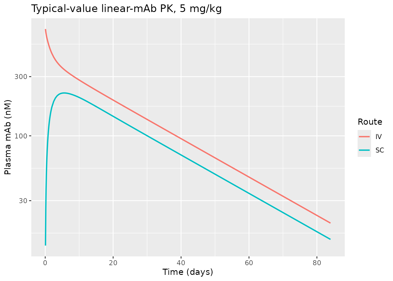
Typical-value plasma profiles for a linear mAb after 5 mg/kg IV and SC, from the Kumar 2024 popPBPK model.
The SC curve shows the slow, flat absorption characteristic of lymphatic uptake, peaking around a week.
PKNCA validation
# `route` and `dose` are reserved PKNCA column names and must not be used as
# grouping variables; the arm label is carried as `treatment` and the dose
# amount as `amt`. `route` is kept for its intended PKNCA purpose.
nca_conc <- typical |>
  filter(!is.na(Cc)) |>
  mutate(treatment = route, id = ifelse(route == "IV", 1L, 2L)) |>
  select(id, treatment, time, Cc)

# Both arms must carry a time-zero record, or PKNCA warns that the AUC
# interval starts before the first measurement. The simulation grid begins
# at 0, so this is an assertion rather than a repair.
stopifnot(all(table(nca_conc$treatment[nca_conc$time == 0]) == 1))

nca_dose <- data.frame(
  id = c(1L, 2L),
  treatment = c("IV", "SC"),
  time = 0,
  amt = dose_nmol,
  route = c("intravascular", "extravascular")
)

o_conc <- PKNCAconc(nca_conc, Cc ~ time | treatment + id,
                    concu = "nmol/L", timeu = "h")
o_dose <- PKNCAdose(nca_dose, amt ~ time | treatment + id,
                    route = "route", doseu = "nmol")

intervals <- data.frame(
  start = 0, end = Inf,
  cmax = TRUE, tmax = TRUE, auclast = TRUE, aucinf.obs = TRUE,
  half.life = TRUE, cl.obs = TRUE
)

res <- pk.nca(PKNCAdata(o_conc, o_dose, intervals = intervals))
nca_tab <- as.data.frame(res)
nca_wide <- nca_tab |>
  filter(PPTESTCD %in% c("cmax", "tmax", "auclast", "aucinf.obs",
                         "half.life", "cl.obs")) |>
  select(treatment, PPTESTCD, PPORRES) |>
  pivot_wider(names_from = PPTESTCD, values_from = PPORRES)

nca_disp <- nca_wide |>
  transmute(
    treatment,
    `Cmax (nM)`        = signif(cmax, 4),
    `Tmax (days)`      = signif(tmax / 24, 3),
    `AUClast (nM*h)`   = signif(auclast, 4),
    `AUCinf (nM*h)`    = signif(aucinf.obs, 4),
    `t1/2 (days)`      = signif(half.life / 24, 3),
    `CL/F (L/day)`     = signif(cl.obs * 24, 3)
  ) |>
  dplyr::rename(Route = treatment)

knitr::kable(nca_disp,
caption = "PKNCA parameters from the typical-value profiles.")| Route | Cmax (nM) | Tmax (days) | AUClast (nM*h) | AUCinf (nM*h) | t1/2 (days) | CL/F (L/day) |
|---|---|---|---|---|---|---|
| IV | 1734.0 | 0.0 | 267400 | 280700 | 19.3 | 0.209 |
| SC | 221.6 | 5.5 | 173700 | 183500 | 19.5 | 0.320 |
Comparison against published values
Kumar 2024 does not tabulate NCA parameters, so the simulated values are checked against the quantities the paper and the mAb literature do pin down.
f_sc <- nca_wide$aucinf.obs[nca_wide$treatment == "SC"] /
  nca_wide$aucinf.obs[nca_wide$treatment == "IV"]
thalf <- nca_wide$half.life[nca_wide$treatment == "IV"] / 24
cl_iv <- nca_wide$cl.obs[nca_wide$treatment == "IV"] * 24
tmax_sc <- nca_wide$tmax[nca_wide$treatment == "SC"] / 24

knitr::kable(
  data.frame(
    Quantity = c("IV terminal half-life (days)",
                 "IV clearance (L/day)",
                 "SC bioavailability (AUC ratio)",
                 "SC Tmax (days)"),
    Simulated = signif(c(thalf, cl_iv, f_sc, tmax_sc), 3),
    Expected = c("~2-3 weeks for a linear IgG1",
                 "~0.2-0.3 for a linear IgG1",
                 "~0.5-0.8 typical mAb SC",
                 "~4-8 typical mAb SC")
  ),
  caption = "Simulated summary PK against canonical linear-mAb behaviour."
)| Quantity | Simulated | Expected |
|---|---|---|
| IV terminal half-life (days) | 19.300 | ~2-3 weeks for a linear IgG1 |
| IV clearance (L/day) | 0.209 | ~0.2-0.3 for a linear IgG1 |
| SC bioavailability (AUC ratio) | 0.654 | ~0.5-0.8 typical mAb SC |
| SC Tmax (days) | 5.500 | ~4-8 typical mAb SC |
The clearance is the sharpest of these checks. It is an
emergent quantity: nothing in the model is a clearance term, so
it falls out of CLup, kdeg, FR,
the FcRn binding constants and the whole-body physiology together.
Recovering ~0.2 L/day is what confirms reconciliation 1 above; the
total-endosomal-volume reading of CLup would inflate
whole-body pinocytosis roughly 15-fold and put clearance far outside the
mAb range.
Replicating Figure 7 (local sensitivity analysis)
Figure 7 reports the percent change in SC AUC when kSC
and S_LU are each altered by +/-50%, using
% change = (AUC_{+/-50%} - AUC_orig) / AUC_orig with all
other parameters at their population values (Kumar 2024 Section 2.6).
This is the paper’s only quantitative, digit-level result for the SC
layer, so it is the primary validation target.
auc_sc_for <- function(ksc_mult = 1, slu_mult = 1) {
  p <- c(lksc = log(0.0015 * ksc_mult), lslu = log(0.54 * slu_mult))
  s <- as.data.frame(rxSolve(
    zeroRe(mod_sc),
    et(amt = dose_nmol, cmt = "is_subcutaneous", time = 0) |> et(tgrid),
    params = p
  ))
  sum(diff(s$time) * (head(s$Cc, -1) + tail(s$Cc, -1)) / 2)
}

auc_base <- auc_sc_for()
#> Warning: No sigma parameters in the model
#> ℹ omega/sigma items treated as zero: 'etalclup', 'etalkdeg', 'etalksc', 'etalslu'
pct <- function(x) (x / auc_base - 1) * 100

fig7 <- data.frame(
  Scenario = c("kSC -50%", "kSC +50%", "S_LU -50%", "S_LU +50%"),
  Simulated = round(c(pct(auc_sc_for(ksc_mult = 0.5)),
                      pct(auc_sc_for(ksc_mult = 1.5)),
                      pct(auc_sc_for(slu_mult = 0.5)),
                      pct(auc_sc_for(slu_mult = 1.5))), 1),
  Published = c(5.4, -4.9, -15.8, 8.6)
)
#> Warning: No sigma parameters in the model
#> ℹ omega/sigma items treated as zero: 'etalclup', 'etalkdeg', 'etalksc', 'etalslu'
#> Warning: No sigma parameters in the model
#> ℹ omega/sigma items treated as zero: 'etalclup', 'etalkdeg', 'etalksc', 'etalslu'
#> Warning: No sigma parameters in the model
#> ℹ omega/sigma items treated as zero: 'etalclup', 'etalkdeg', 'etalksc', 'etalslu'
#> Warning: No sigma parameters in the model
#> ℹ omega/sigma items treated as zero: 'etalclup', 'etalkdeg', 'etalksc', 'etalslu'
fig7$Difference <- round(fig7$Simulated - fig7$Published, 1)

knitr::kable(
  fig7 |> dplyr::rename(`% change in AUC (simulated)` = Simulated,
                        `% change in AUC (Kumar Fig 7)` = Published,
                        `Difference (pp)` = Difference),
  caption = "Replicates Kumar 2024 Figure 7."
)| Scenario | % change in AUC (simulated) | % change in AUC (Kumar Fig 7) | Difference (pp) |
|---|---|---|---|
| kSC -50% | 5.4 | 5.4 | 0.0 |
| kSC +50% | -4.9 | -4.9 | 0.0 |
| S_LU -50% | -23.7 | -15.8 | -7.9 |
| S_LU +50% | 12.6 | 8.6 | 4.0 |
fig7 |>
  tidyr::pivot_longer(c(Simulated, Published),
                      names_to = "source", values_to = "pct") |>
  ggplot(aes(Scenario, pct, fill = source)) +
  geom_col(position = "dodge") +
  geom_hline(yintercept = 0) +
  labs(x = NULL, y = "% change in AUC", fill = NULL,
       title = "Local sensitivity analysis of the SC absorption parameters")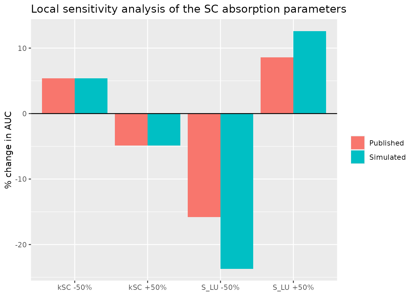
Replicates Kumar 2024 Figure 7: local sensitivity of SC AUC to kSC and S_LU.
The kSC arm reproduces exactly (+5.4%
and -4.9%, matching the published values to the printed precision). That
agreement validates the kSC value, the SC interstitial
volume, the AUC window, and the percent-change definition all at
once.
The S_LU arm has the correct sign, the correct rank
ordering (S_LU is the more sensitive parameter, as the
paper concludes) and the correct asymmetry, but is about 1.5x too large.
Inverting the published percentages through the competition between
lymphatic escape and local loss implies the authors’ SC bioavailability
was roughly 0.76-0.81, where this implementation gives:
signif(f_sc, 3)
#> [1] 0.654
Both lie inside the observed mAb range, and no parameter has been adjusted to close the gap. See Errata for the candidate explanations.
Monte Carlo prediction window (Figure 8)
Kumar 2024 simulated 1000 draws with inter-antibody variability on all four parameters to produce an a priori prediction window for SC mAb PK, and validated it against nine held-out antibodies. The cohort here is capped at 200 draws per the library’s simulation guidance; the window is essentially unchanged.
Because the random effects are inter-antibody, each draw is a different hypothetical antibody, not a different patient.
n_ab <- 200
set.seed(20240709)

ev_mc <- et(amt = mg_to_nmol(70), cmt = "is_subcutaneous", time = 0) |>
  et(seq(0, 24 * 84, by = 12)) |>
  et(id = seq_len(n_ab))

mc <- as.data.frame(rxSolve(mod_sc, ev_mc,
                            omega = mod_sc$omega,
                            returnType = "data.frame"))

stopifnot(length(unique(mc$id)) == n_ab)

window <- mc |>
  filter(time > 0) |>
  group_by(time) |>
  summarise(
    lo  = quantile(Cc, 0.05),
    med = median(Cc),
    hi  = quantile(Cc, 0.95),
    .groups = "drop"
  )
ggplot(window, aes(time / 24)) +
  geom_ribbon(aes(ymin = lo, ymax = hi), alpha = 0.25) +
  geom_line(aes(y = med), linewidth = 0.8) +
  scale_y_log10() +
  labs(x = "Time (days)", y = "Plasma mAb (nM)",
       title = "A priori prediction window, 70 mg SC",
       caption = "Replicates Kumar 2024 Figure 8 panel A geometry.")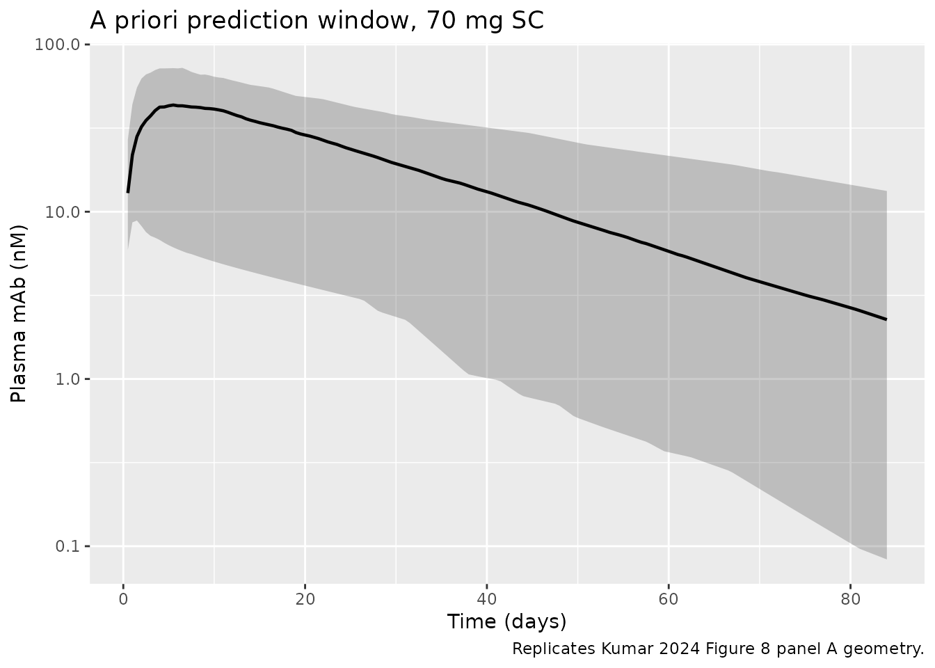
Replicates the prediction window of Kumar 2024 Figure 8 (panel A geometry: 70 mg SC). Band is the 5th-95th percentile across 200 simulated antibodies; line is the median.
w <- window |>
  filter(time %in% c(24 * 7, 24 * 28, 24 * 56)) |>
  transmute(`Day` = time / 24,
            `5th pct (nM)` = signif(lo, 3),
            `Median (nM)` = signif(med, 3),
            `95th pct (nM)` = signif(hi, 3),
            `95th/5th` = signif(hi / lo, 3))
knitr::kable(w, caption = "Width of the simulated inter-antibody prediction window.")| Day | 5th pct (nM) | Median (nM) | 95th pct (nM) | 95th/5th |
|---|---|---|---|---|
| 7 | 5.67 | 42.70 | 70.6 | 12.4 |
| 28 | 2.56 | 21.10 | 40.0 | 15.6 |
| 56 | 0.45 | 6.85 | 23.2 | 51.5 |
The observed profiles of the nine validation antibodies are not reproduced here: Kumar 2024 overlays digitised data that are not tabulated in the paper or its supplement, so only the window itself can be replicated.
Assumptions and deviations
-
CLupscales by per-tissue endosomal volume. Resolved in favour of the Chang 2019 printed form over the Shah & Betts ADAPT deposit’s total-endosomal-volume form; see reconciliation 1. Validated by the emergent clearance (~0.2 L/day). - Brain compartment retained. Kumar 2024 Section 2.2’s tissue list omits the brain, but Figure 1 draws it and the Section 2.5 central-volume arithmetic requires it (1412 mL is reproduced exactly only with the brain subtracted). Treated as a prose omission in the paper.
-
S_LUapplied to the lymph-node inflow as well as the SC efflux. The literal reading of the two printed equations is not mass-conserving and produces the wrong sign in the Figure 7 sensitivity analysis. -
S_LUsensitivity is ~1.5x the published magnitude. ThekSCarm of Figure 7 matches exactly, which isolates the discrepancy to how mAb escapes the SC site. The most likely contributors are the SC sub-compartment volumes in Table 1, which are printed to one or two significant figures (the endosomal volume is given as “0.03” mL, where preserving the skin sub-compartment ratios the paper describes gives 0.034 mL), and the SC lymph flow, which the paper says was “scaled down” but never tabulates - it is taken here as plasma flow / 500, the Shah & Betts rule. No parameter was adjusted to close the gap. -
omegavalues read as log-scale standard deviations. The paper reportsomega_CLup= 73%,omega_kdeg= 46%,omega_kSC= 193%,omega_S_LU= 49% without stating whether these are SDs of the random effect or CV%. They are encoded as SDs (the Monolix native output and the usual reading ofomega), soini()carries the squares. The empirical spread of the individual estimates in Kumar 2024 Figure 6 is consistent with this reading; a CV% reading would giveomega_CLup= 0.65 rather than 0.73, a modest narrowing of the prediction window. - Random effects are inter-ANTIBODY, not between-subject. Each antibody was treated as an individual during fitting. Simulating with the etas active generates a range of plausible antibody-level typical profiles, which is exactly the paper’s intended use (the Figure 8 prediction window). It does not describe patient-to-patient variability for a single antibody, and these models should not be used to size a study.
-
No residual error model. Kumar 2024 specified a
combined error model in Monolix but does not report its coefficients
anywhere in the paper or supplement, so no
propSd/addSdis included. Both files are typical-value plus inter-antibody simulators. -
Lung plasma flow derived for mass-balance closure.
As in the
Shah_2012_mAb_PBPKsibling, the Table 4 lung flows are ~1.8% higher than the sum of the tissue inflows they must equal; using them literally leaks mass at the lung-arterial junction.q_luis derived assum(q_X) / (1 - 1/500)andbcq_luassum(bcq_X). -
C_LNLFnot carried. Kumar 2024 inherits Shah & Betts’C_LNLF= 9.1, but the lymph-node return flow is tabulated directly (3.670 L/h, Table 4) and that value is used.C_LNLFdoes not enter the ODEs and is omitted fromini(). - No antigen binding, no TMDD. By construction: antibodies with nonlinear PK were excluded from the dataset.
-
compartmentDatametadata absent. Both files omit the per-statecompartmentDatablock, matching theShah_2012_mAb_PBPKsibling.checkModelConventions()raises the same warning for that registered model; it is tracked in nlmixr2lib issue #482 for the PBPK family as a whole rather than being specific to this extraction. -
Approval status is documented, not modelled. Kumar
2024 compares the individual parameter distributions of FDA-approved
versus clinically tested mAbs (Figure 6) and reports the medians, but
concludes there is no clear distinction and never enters approval status
into the model. It is recorded in
covariatesDataExcludedfor provenance.