Flip-flop and local identifiability (Kuan 2023)
Source:vignettes/articles/Kuan_2023_flipflop.Rmd
Kuan_2023_flipflop.RmdModel and source
- Citation: Kuan IHS, Wright DFB, Duffull SB. The influence of flip-flop in population pharmacokinetic analyses. CPT Pharmacometrics Syst Pharmacol. 2023;12(3):285-287. doi:10.1002/psp4.12909. PMID 36647235. PMCID PMC10014047. Parameter values transcribed from Supplement Appendix S1 Table S1 (Permutation 1 column); the permutation algebra is main-text Table 1.
- Article: https://doi.org/10.1002/psp4.12909
- Supplement (Appendices S1-S3): https://doi.org/10.1002/psp4.12909, Supporting Information
This paper contributes two model files, one per permutation of the same one-compartment model:
-
Kuan_2023_oral1cmt_permutation1– theka > kbranch. -
Kuan_2023_oral1cmt_permutation2– theka < kbranch.
m1 <- rxode2::rxode(readModelDb("Kuan_2023_oral1cmt_permutation1"))
m2 <- rxode2::rxode(readModelDb("Kuan_2023_oral1cmt_permutation2"))

tibble::tibble(
  Model = c("Kuan_2023_oral1cmt_permutation1", "Kuan_2023_oral1cmt_permutation2"),
  ka    = c(exp(m1$theta[["lka"]]), exp(m2$theta[["lka"]])),
  V     = c(exp(m1$theta[["lvc"]]), exp(m2$theta[["lvc"]])),
  CL    = c(exp(m1$theta[["lcl"]]), exp(m2$theta[["lcl"]]))
) |>
  mutate(k = CL / V) |>
  relocate(k, .after = ka) |>
  knitr::kable(
    digits  = 3,
    caption = "Appendix S1 Table S1. Both permutations of the one-compartment model."
)| Model | ka | k | V | CL |
|---|---|---|---|---|
| Kuan_2023_oral1cmt_permutation1 | 0.5 | 0.1 | 10 | 1 |
| Kuan_2023_oral1cmt_permutation2 | 0.1 | 0.5 | 2 | 1 |
What the paper is about
“Flip-flop” describes a model whose absorption and elimination rate
constants appear to be switched. Kuan 2023 argues that this is not
really a switch but a permutation of the rank order of the
parameter values, and therefore an issue of local
identifiability: a finite set of parameter vectors – not a single
one – reproduces the same input-output relationship. For a mammillary
model with n compartments and a depot, there are
n + 1 such permutations.
The one-compartment case has two, and Appendix S1 Table S1 gives both numerically. The whole point of this vignette is that those two parameter sets must produce the same concentration-time curve.
Population
There is no population. Both model files encode an author-chosen
mathematical demonstration – no drug, no patients, no fitted estimates –
so every value is wrapped in fixed(). This follows the
precedent of Beal_2001_iv1cmt_bql, the other
methodology-reference toy model in the library.
str(m1$population)
#> List of 7
#>  $ species      : chr "None (methodology paper; a single deterministic simulated profile of a hypothetical drug, not a fit of any real molecule)."
#>  $ n_subjects   : int 1
#>  $ disease_state: chr "N/A (algebraic demonstration of local identifiability)."
#>  $ dose_range   : chr "Single unit dose, D = 1, with F = 1 (Appendix S1 Table S1)."
#>  $ regions      : chr "N/A"
#>  $ scope_note   : chr "Filed under inst/modeldb/pharmacokinetics/ rather than specificDrugs/ because there is no drug, following the p"| __truncated__
#>  $ notes        : chr "Appendix S1: 'Simulations using all the possible permutations for a one-compartment model was performed to illu"| __truncated__
The paper’s motivating analysis (main text and Appendix S3) is a separate metformin population fit: 55 participants contributing 426 plasma concentrations pooled from Kuan 2021, Dissanayake 2017 and Pentikainen 1979, with creatinine clearance (Cockcroft-Gault, computed on ideal body weight) spanning 9.5 to 167.0 mL/min. That model is not encodable and is not included here – see Errata below.
Source trace
| Equation / parameter | Value | Source location |
|---|---|---|
| Structural model | 1-compartment, first-order in and out | Main text, p. 286 (“A one-compartment with first-order input and output model was fit to the data”); Appendix S1 |
lka (permutation 1) |
log(0.5) |
Appendix S1 Table S1, Permutation 1: ka = 0.5
|
lvc (permutation 1) |
log(10) |
Appendix S1 Table S1, Permutation 1: V = 10
|
lcl (permutation 1) |
log(1) |
Derived: CL = V * k = 10 * 0.1; Table S1 gives
k = 0.1. Main text p. 286: “CL remains unchanged in both
permutations and is therefore invariant to flip-flop” |
lfdepot (permutation 1) |
log(1) |
Appendix S1 Table S1, Permutation 1: F = 1
|
lka (permutation 2) |
log(0.1) |
Appendix S1 Table S1, Permutation 2: ka = 0.1
|
lvc (permutation 2) |
log(2) |
Appendix S1 Table S1, Permutation 2: V = 2
|
lcl (permutation 2) |
log(1) |
Derived: CL = V * k = 2 * 0.5; Table S1 gives
k = 0.5
|
lfdepot (permutation 2) |
log(1) |
Appendix S1 Table S1, Permutation 2: F = 1
|
| Dose |
D = 1 at time = 0
|
Appendix S1 Table S1 |
| Observation grid | t = 0:100 |
Appendix S1 Table S1 |
| 1-cmt permutation algebra | see below | Main text Table 1 |
| 2-cmt permutation algebra | see below | Main text Table 1; Appendix S2 |
Virtual cohort
The source simulation is deterministic: one profile per permutation, no between-subject variability and no residual error (none is reported, so none is encoded). The “cohort” is therefore two single profiles, far below the 200-per-arm cap.
# Appendix S1 Table S1 specifies t = 0:100. A step of 0.1 rather than 1 is used
# so that the trapezoidal NCA below resolves Tmax (analytically 4.02); the
# plotted curve is unaffected. See "Assumptions and deviations".
tgrid <- seq(0, 100, by = 0.1)

events <- rxode2::et(amt = 1, cmt = "depot", time = 0) |>
  rxode2::et(time = tgrid, cmt = "central")
Note that observation rows use cmt = "central" – the ODE
state – not the algebraic observable Cc; rxode2 returns
Cc as a column regardless.
Simulation
# Neither model declares an eta, so `omega = NA` must NOT be passed (it would
# fail in rep(0, dim(NA)[1])), and zeroRe() is unnecessary.
solve_perm <- function(mod, label) {
  # Tight solver tolerances: the gates below hold two numerically integrated
  # profiles to each other and to the closed form at 1e-8 / 1e-10.
  rxode2::rxSolve(mod, events = events, rtol = 1e-10, atol = 1e-12) |>
    as.data.frame() |>
    # rxSolve omits `id` for a single-subject event table; PKNCA needs it.
    mutate(id = 1L, permutation = label)
}

sim <- bind_rows(
  solve_perm(m1, "Permutation 1"),
  solve_perm(m2, "Permutation 2")
)

stopifnot(
  nrow(sim) == 2 * length(tgrid),
  !anyNA(sim$Cc),
  # PKNCA takes log() of the tail; a solve that dipped negative would give NaN.
  all(sim$Cc >= 0)
)
Replicate Figure S1
# Replicates Figure S1 of Kuan 2023: "Simulations of the permutations that
# provide the same input-output relationship for a one compartment
# pharmacokinetic model." The curves are plotted with different linetypes and
# widths so that the (exact) overlap is visible rather than one hiding the other.
ggplot(sim, aes(time, Cc, colour = permutation, linetype = permutation)) +
  geom_line(aes(linewidth = permutation)) +
  scale_linewidth_manual(values = c("Permutation 1" = 1.6, "Permutation 2" = 0.6)) +
  scale_linetype_manual(values = c("Permutation 1" = "solid", "Permutation 2" = "22")) +
  coord_cartesian(xlim = c(0, 60)) +
  labs(
    x = "Time (time_unit)", y = "Cc (dose_unit / vol_unit)",
    title = "Figure S1 - the two permutations superimpose",
    caption = "Replicates Figure S1 of Kuan 2023."
  ) +
  theme(legend.position = "bottom")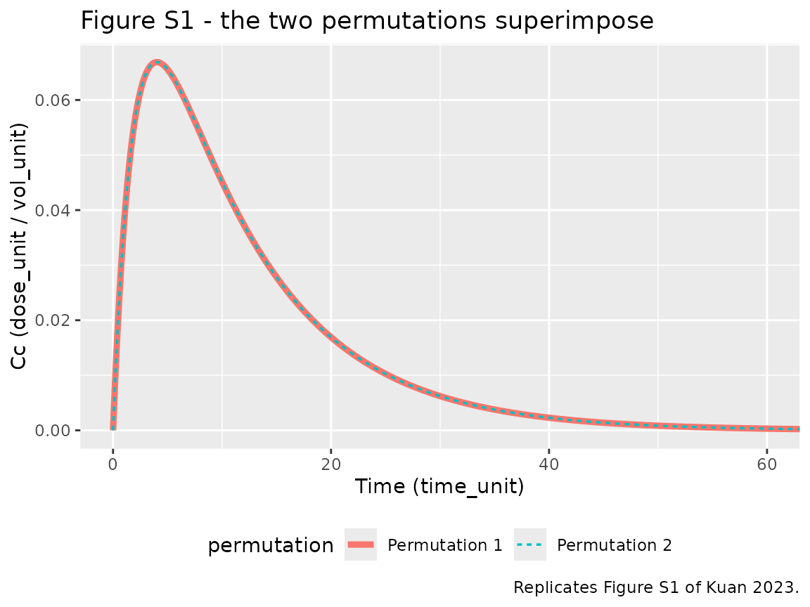
Validation
Every check below is deterministic – there is no random effect anywhere in either model, so both sides of each comparison are exact solves of the same system and the only difference is numerical. Tight tolerances are therefore correct here, and are deliberately not the loose cohort-quantile bounds used in vignettes that simulate a random population.
Gate 1: the permutations superimpose (the paper’s central claim)
w <- sim |>
  select(time, permutation, Cc) |>
  pivot_wider(names_from = permutation, values_from = Cc)

abs_diff <- max(abs(w$`Permutation 1` - w$`Permutation 2`))
big      <- w$`Permutation 1` > 1e-6
rel_diff <- max(abs((w$`Permutation 1` - w$`Permutation 2`) / w$`Permutation 1`)[big])

c(max_abs_difference = abs_diff, max_relative_difference = rel_diff)
#>      max_abs_difference max_relative_difference
#>            1.927555e-12            3.972251e-10

# Achieved 1.9e-12 (absolute) and 4.0e-10 (relative) with the ODE integrator at
# rtol 1e-10 / atol 1e-12 (4.9e-17 / 3.0e-15 under the analytic linCmt path).
# Bound set well above that but still far below any real structural error --
# a single mis-transcribed parameter moves these to O(1).
stopifnot(abs_diff < 1e-10, rel_diff < 1e-8)
Gate 2: each permutation matches the analytic solution
# C(t) = F * D * ka / (V * (ka - k)) * (exp(-k t) - exp(-ka t))
Canalytic <- function(t, F, D, ka, k, V) {
  (F * D * ka) / (V * (ka - k)) * (exp(-k * t) - exp(-ka * t))
}

closed_form <- sim |>
  group_by(permutation) |>
  mutate(
    Cref = Canalytic(
      time, F = 1, D = 1,
      ka = first(ka), k = first(kel), V = first(vc)
    )
  ) |>
  summarise(
    max_abs_error = max(abs(Cc - Cref)),
    max_rel_error = max((abs(Cc - Cref) / Cref)[Cref > 1e-6]),
    .groups = "drop"
  )

knitr::kable(closed_form, digits = 20,
caption = "Numerical solve vs. the closed-form solution.")| permutation | max_abs_error | max_rel_error |
|---|---|---|
| Permutation 1 | 5.385553e-13 | 2.498681e-11 |
| Permutation 2 | 1.982825e-12 | 4.086150e-10 |
# Achieved <= 2.0e-12 absolute / <= 4.1e-10 relative for both permutations with
# the ODE integrator at rtol 1e-10 / atol 1e-12 (~2e-16 / ~5e-14 analytic).
stopifnot(closed_form$max_abs_error < 1e-10, closed_form$max_rel_error < 1e-8)
Gate 3: main-text Table 1, one-compartment permutation algebra
Table 1 states the permutation rules in two parameterizations. Applying them to permutation 1 must reproduce permutation 2 exactly.
ka <- 0.5; V <- 10; k <- 0.1        # Table S1, Permutation 1
CL <- V * k

t1 <- tibble::tibble(
  Parameterization = c("(k, V, ka)", "(k, V, ka)", "(k, V, ka)",
                       "(CL, V, ka)", "(CL, V, ka)", "(CL, V, ka)"),
  Rule = c("k' = ka", "V' = (V * k) / ka", "ka' = k",
           "CL' = CL", "V' = CL / ka", "ka' = CL / V"),
  Derived  = c(ka, (V * k) / ka, k, CL, CL / ka, CL / V),
  Expected = c(0.5, 2, 0.1, 1, 2, 0.1)   # Table S1 Permutation 2 (CL = V * k = 2 * 0.5)
)

knitr::kable(t1, digits = 6,
caption = "Table 1 permutation rules applied to Permutation 1.")| Parameterization | Rule | Derived | Expected |
|---|---|---|---|
| (k, V, ka) | k’ = ka | 0.5 | 0.5 |
| (k, V, ka) | V’ = (V * k) / ka | 2.0 | 2.0 |
| (k, V, ka) | ka’ = k | 0.1 | 0.1 |
| (CL, V, ka) | CL’ = CL | 1.0 | 1.0 |
| (CL, V, ka) | V’ = CL / ka | 2.0 | 2.0 |
| (CL, V, ka) | ka’ = CL / V | 0.1 | 0.1 |
Note the asymmetry the paper highlights: under
(k, V, ka) the permutation is complete – the two rate
constants simply exchange – whereas under (CL, V, ka)
clearance is unchanged, and it is V and
ka that are functions of the other parameters. Clearance is
the flip-flop invariant.
Gate 4: Table 1 / Appendix S2, two-compartment permutation algebra
The two-compartment model has n + 1 = 3 permutations.
The paper gives these symbolically only (Table 1 and the substitutions
of Appendix S2) with no numeric values, so no model
file is generated for this case. The identity can still be checked: the
values below are chosen here purely to evaluate the paper’s algebra and
are not from the paper.
C2 <- function(t, F, D, ka, alpha, beta, k21, Vc) {
  (F * D * ka / Vc) * (
    (k21 - alpha) * exp(-alpha * t) / ((ka - alpha) * (beta - alpha)) +
    (k21 - beta)  * exp(-beta  * t) / ((ka - beta)  * (alpha - beta)) +
    (k21 - ka)    * exp(-ka    * t) / ((alpha - ka) * (beta - ka))
  )
}

tt <- seq(0, 60, by = 0.05)
ka2 <- 0.3; alpha <- 1.0; beta <- 0.1; k21 <- 0.2; Vc <- 5
# Sanity: a valid 2-cmt disposition requires beta < k21 < alpha and k10, k12 > 0.
stopifnot(beta < k21, k21 < alpha,
          alpha * beta / k21 > 0,
          alpha + beta - k21 - alpha * beta / k21 > 0)

p1 <- C2(tt, 1, 1, ka2,  alpha, beta,  k21, Vc)
# Permutation 2: alpha' = ka, beta' = beta, ka' = alpha, Vc' = Vc * alpha / ka
p2 <- C2(tt, 1, 1, alpha, ka2,  beta,  k21, Vc * alpha / ka2)
# Permutation 3: alpha' = alpha, beta' = ka, ka' = beta, Vc' = Vc * beta / ka
p3 <- C2(tt, 1, 1, beta,  alpha, ka2,   k21, Vc * beta / ka2)

relmax <- function(x, y) max((abs(x - y) / abs(y))[abs(y) > 1e-9])
two_cmt <- c(perm2_vs_perm1 = relmax(p2, p1), perm3_vs_perm1 = relmax(p3, p1))
two_cmt
#> perm2_vs_perm1 perm3_vs_perm1
#>   1.227647e-15   2.308361e-16

# Achieved 1.2e-15 and 2.3e-16.
stopifnot(all(two_cmt < 1e-8))
PKNCA validation
The paper makes a specific, testable claim about noncompartmental analysis (main text, p. 286):
“noncompartmental analyses are unaffected by a model being in either a ‘flip’ or a ‘flop’ state”
and
“the standard exposure relationship
AUC = Dose/CLremains true irrespective of whether the system is in a state of ‘flip’ or ‘flop’”.
NCA is therefore the right validation tool here, and the gate is that every NCA parameter must be identical across the two permutations.
sim_nca <- sim |>
  dplyr::filter(!is.na(Cc)) |>
  dplyr::select(id, time, Cc, permutation)

# Guarantee a time = 0 row per (id, permutation); pre-dose Cc = 0 extravascular.
sim_nca <- dplyr::bind_rows(
  sim_nca,
  sim_nca |> dplyr::distinct(id, permutation) |> dplyr::mutate(time = 0, Cc = 0)
) |>
  dplyr::distinct(id, permutation, time, .keep_all = TRUE) |>
  dplyr::arrange(permutation, id, time)

conc_obj <- PKNCA::PKNCAconc(sim_nca, Cc ~ time | permutation + id)

dose_df <- sim_nca |>
  dplyr::distinct(id, permutation) |>
  dplyr::mutate(time = 0, amt = 1)
dose_obj <- PKNCA::PKNCAdose(dose_df, amt ~ time | permutation + id)

# Two intervals. The terminal-slope interval starts at t = 40 because a
# lambda.z window opening just after Tmax still contains the fast exponential
# and biases the estimate (0.0997 rather than 0.1000, so half-life reads 6.95
# instead of 6.93). By t = 40 the fast term has decayed to ~1e-6 of the slow
# one. Fit the terminal slope well clear of the
# distribution phase.
intervals <- data.frame(
  start      = c(0, 40),
  end        = c(Inf, Inf),
  cmax       = c(TRUE,  FALSE),
  tmax       = c(TRUE,  FALSE),
  aucinf.obs = c(TRUE,  FALSE),
  cl.obs     = c(TRUE,  FALSE),
  half.life  = c(FALSE, TRUE),
  lambda.z   = c(FALSE, TRUE)
)

nca_res <- suppressWarnings(
  PKNCA::pk.nca(PKNCA::PKNCAdata(conc_obj, dose_obj, intervals = intervals))
)

nca_tidy <- as.data.frame(nca_res) |>
  # lambda.z / half.life are computed on BOTH intervals (aucinf needs lambda.z);
  # keep the terminal-window value for those and the full-window value otherwise.
  dplyr::filter(
    (PPTESTCD %in% c("half.life", "lambda.z") & start == 40) |
      (PPTESTCD %in% c("cmax", "tmax", "aucinf.obs", "cl.obs") & start == 0)
  ) |>
  dplyr::select(permutation, PPTESTCD, PPORRES)

stopifnot(nrow(nca_tidy) == 12L)   # 6 parameters x 2 permutations; guards against a vacuous pass
NCA is invariant to the permutation
nca_wide <- nca_tidy |>
  pivot_wider(names_from = permutation, values_from = PPORRES)

nca_wide |>
  mutate(`Absolute difference` = abs(`Permutation 1` - `Permutation 2`)) |>
  dplyr::rename("NCA parameter" = PPTESTCD) |>
  knitr::kable(digits = 10,
caption = "Every NCA parameter is identical across permutations.")| NCA parameter | Permutation 1 | Permutation 2 | Absolute difference |
|---|---|---|---|
| cmax | 0.0668731 | 0.0668731 | 0 |
| tmax | 4.0000000 | 4.0000000 | 0 |
| aucinf.obs | 0.9999535 | 0.9999535 | 0 |
| cl.obs | 1.0000465 | 1.0000465 | 0 |
| lambda.z | 0.1000000 | 0.1000000 | 0 |
| half.life | 6.9314718 | 6.9314718 | 0 |
Simulated NCA against the analytic reference
The paper reports no NCA table, so the reference column below is the analytic value implied by the paper’s own Table S1 parameters, not a transcribed published number.
val <- function(p) nca_wide$`Permutation 1`[nca_wide$PPTESTCD == p]

cmp <- tibble::tibble(
  `NCA parameter` = c("Cmax", "Tmax", "AUC0-inf (obs)", "CL/F (obs)", "t-half", "lambda-z"),
  Simulated = c(val("cmax"), val("tmax"), val("aucinf.obs"),
                val("cl.obs"), val("half.life"), val("lambda.z")),
  `Analytic reference` = c(
    Canalytic(log(0.5 / 0.1) / (0.5 - 0.1), 1, 1, 0.5, 0.1, 10),  # Cmax
    log(0.5 / 0.1) / (0.5 - 0.1),                                  # Tmax
    1,                                                             # AUC = Dose/CL = 1/1
    1,                                                             # CL = V * k = 1
    log(2) / 0.1,                                                  # slower rate constant
    0.1                                                            # slower rate constant
  ),
  Source = c(
    "Closed form at Tmax", "ln(ka/k)/(ka-k)",
    "Dose/CL, main text p. 286", "Table S1: CL = V * k",
    "ln(2)/0.1", "the SLOWER of ka and k"
  )
) |>
  mutate(`Percent difference` = 100 * (Simulated - `Analytic reference`) /
           `Analytic reference`)

knitr::kable(cmp, digits = 6,
caption = "Simulated NCA vs. the analytic values implied by Table S1.")| NCA parameter | Simulated | Analytic reference | Source | Percent difference |
|---|---|---|---|---|
| Cmax | 0.066873 | 0.066874 | Closed form at Tmax | -0.001398 |
| Tmax | 4.000000 | 4.023595 | ln(ka/k)/(ka-k) | -0.586410 |
| AUC0-inf (obs) | 0.999953 | 1.000000 | Dose/CL, main text p. 286 | -0.004652 |
| CL/F (obs) | 1.000047 | 1.000000 | Table S1: CL = V * k | 0.004652 |
| t-half | 6.931472 | 6.931472 | ln(2)/0.1 | 0.000000 |
| lambda-z | 0.100000 | 0.100000 | the SLOWER of ka and k | 0.000000 |
# Tmax is exempt from the percentage gate: the observation grid has a 0.1 step
# and the true Tmax is 4.0236, so the grid maximum necessarily lands at 4.0.
# That is a discretisation artefact of the sampling schedule, not a model
# error, and the honest assertion is that it agrees to within one grid step.
tight <- cmp |> dplyr::filter(`NCA parameter` != "Tmax")

# Achieved: 0.0047 percent (AUC and CL/F), 0.0014 percent (Cmax), 4e-7 percent
# (half-life, lambda.z). These are trapezoidal-discretisation errors on a fixed
# grid, not solver noise, so they are reproducible -- but the bound is set an
# order of magnitude above the worst of them so that a future PKNCA AUC-method
# change does not turn this red. It still goes red loudly for what it is meant
# to catch: a mis-transcribed CL, V, ka or dose moves these by tens of percent.
stopifnot(max(abs(tight$`Percent difference`)) < 0.05)

tmax_sim <- cmp$Simulated[cmp$`NCA parameter` == "Tmax"]
tmax_ref <- cmp$`Analytic reference`[cmp$`NCA parameter` == "Tmax"]
stopifnot(abs(tmax_sim - tmax_ref) <= 0.1 + 1e-12)   # within one observation-grid step
Both permutations return AUC0-inf = 1 and
CL/F = 1, confirming AUC = Dose/CL in each
state, and both return the same terminal half-life – because the
terminal slope always recovers the slower of the two
rate constants, which is k = 0.1 under permutation 1 and
ka = 0.1 under permutation 2. That is precisely the
flip-flop ambiguity, and it is invisible to NCA.
What NCA does not recover
Clearance is invariant, but volume is not: Table 1 gives
V' = V * k / ka, so the two permutations have genuinely
different volumes (10 and 2). The usual NCA volume
Vz = CL / lambda_z returns a single number, which can only
be right for one of them.
Vz <- val("cl.obs") / val("lambda.z")

tibble::tibble(
  Quantity = c("Vz from NCA (both permutations)",
               "True V, permutation 1", "True V, permutation 2"),
  Value = c(Vz, exp(m1$theta[["lvc"]]), exp(m2$theta[["lvc"]]))
) |>
  knitr::kable(digits = 4,
caption = "Volume is permuted by flip-flop; NCA cannot resolve it.")| Quantity | Value |
|---|---|
| Vz from NCA (both permutations) | 10.0005 |
| True V, permutation 1 | 10.0000 |
| True V, permutation 2 | 2.0000 |
Assumptions and deviations
-
Observation grid. Appendix S1 Table S1 specifies
t = 0:100. A step of 0.1 rather than 1 is used so trapezoidal NCA resolvesTmax = 4.02; on a unit grid the AUC is understated. The plotted profile is unchanged, and the closed-form gates hold on either grid. -
Clearance is derived, not printed. Table S1 reports
kandV; the model files store the canonical(CL, V, ka)parameterization withCL = V * k = 1. Both permutations therefore carrylcl = log(1), which is the paper’s own invariance claim made explicit in theini()block. The paper’skis recovered inmodel()askel = cl / vc. - No IIV and no residual error are encoded, because the Appendix S1 demonstration is deterministic and reports none. The metformin model (Appendix S3) is described as using exponential between-subject variability and a combined residual error model, but no variance or error value is given for either.
-
Terminal-slope window.
lambda.zis fit fromt = 40rather than from the default post-Tmax window, which would still contain the fast exponential and bias half-life by about 0.3 percent. -
The two-compartment check uses non-paper values.
Gate 4 evaluates the paper’s Table 1 / Appendix S2 algebra at
ka = 0.3,alpha = 1.0,beta = 0.1,k21 = 0.2,Vc = 5. These were chosen for this vignette solely to evaluate an identity the paper states symbolically; they appear in no model file and are not attributable to the authors. -
Compartment metadata is unverified
(
verified = FALSE). Appendix S1 names no molecule and no biological matrix, soanalyteandspecimencannot be confirmed against the source.
Errata and scope
-
The metformin population model is not extractable.
The main text and Appendix S3 describe it in full – data sources, BQL
handling (M6 per Beal 2001), NONMEM 7.3 with FOCE-I, a one-compartment
structure, exponential BSV, combined residual error, and a
creatinine-clearance covariate screen on
kaand onCL– but report no parameter estimate of any kind. There is no fixed-effect value, no OMEGA, no SIGMA and no covariate coefficient anywhere in the paper or its supplement; only the direction of the objective-function change is stated. Nothing can be placed in anini()block, so no metformin model file is generated. The covariate screen is preserved ascovariatesDataExcluded$CRCLin both model files. -
Related metformin models already in the library.
The paper’s own data sources are separately published.
Chae_2012_metformin,Choi_2018_metformin,vanRongen_2018_metforminandYoon_2013_metforminare already packaged; the upstream source for this paper’s largest cohort, Kuan 2021 (PLOS One, doi:10.1371/journal.pone.0246247), is not, and is the natural candidate for a future extraction. - No erratum. No correction or corrigendum was found for doi:10.1002/psp4.12909.
-
Article type. This is a three-page
Perspective. It is extracted because Appendix S1 Table S1 fully
specifies a numeric model, matching the precedent set by
Beal_2001_iv1cmt_bql(a methodology paper’s simulation-only toy model, filed underpharmacokinetics/by maintainer decision).