Generic perfusion-limited whole-body PBPK template (Jones 2013)
Source:vignettes/articles/Jones_2013_perfusionLimited_pbpk.Rmd
Jones_2013_perfusionLimited_pbpk.RmdModel and source
- Citation: Jones HM, Rowland-Yeo K. Basic concepts in physiologically based pharmacokinetic modeling in drug discovery and development. CPT Pharmacometrics Syst Pharmacol. 2013;2(8):e63. doi:10.1038/psp.2013.41. PMID 23945604. PMCID PMC3828005. The model is transcribed in full from the Supplementary Data file (psp201341x1.doc), sections {HUMAN PBPK MODEL}, {SPECIES SPECIFIC PARAMETERS}, {COMPOUND SPECIFIC PARAMETERS} and {DOSING}; the main-text narrative of the perfusion-limited mass balance is Equations 1 and 2 and the microsomal clearance scaling is Equation 3. See the vignette Errata for the one divergence between the main-text equation and the deposited code.
- Article: CPT Pharmacometrics Syst Pharmacol 2013;2(8):e63 (PMC3828005, CC BY-NC-ND).
- Supplement:
psp201341x1.doc, published with the open-access article (PMC3828005). It contains one Berkeley Madonna listing headed{HUMAN PBPK MODEL}followed by{SPECIES SPECIFIC PARAMETERS},{COMPOUND SPECIFIC PARAMETERS}and{DOSING}.
This is a tutorial paper, and the model extracted here is the one the authors deposited rather than either of the two worked examples in the main text. The distinction matters, so it is worth stating plainly:
- The main text’s Example 1 (an anonymised “compound X”) and Example 2 (repaglinide) were both run on the Simcyp Population-Based Simulator. Neither is reproducible from the paper: the tissue-to-plasma partition coefficients, the ADAM absorption model and – for repaglinide – the permeability-limited liver sub-compartment geometry are all vendor-internal and are not printed. Only physicochemical inputs (Tables 1 and 3) and observed-versus-predicted summaries (Table 2) appear. Those two examples are therefore not extracted.
- The Supplementary Data, by contrast, is a complete and platform-free model. Every constant its equations consume is printed: fifteen fractional tissue volumes, thirteen fractional blood flows, a cardiac output, a body weight, thirteen partition coefficients, three binding parameters, MPPGL, a microsomal intrinsic clearance, a renal clearance, and the two absorption parameters. That is what this vignette validates.
The compound is deliberately neutral: every Kp, the
blood-to-plasma ratio and both unbound fractions are set to exactly 1.
The file is a template into which a real compound’s
predicted Kp vector, binding data and intrinsic clearance
are substituted. As shown below, that neutrality also makes the model’s
exposure analytically solvable, which is what lets this vignette check
the transcription against closed forms rather than against a digitised
figure.
mod <- rxode2::rxode2(readModelDb("Jones_2013_perfusionLimited_pbpk"))
length(mod$state)
#> [1] 16
mod$state
#>  [1] "depot"    "adipose"  "bone"     "brain"    "gut"      "heart"
#>  [7] "kidney"   "liver"    "lung"     "muscle"   "skin"     "spleen"
#> [13] "testes"   "venous"   "arterial" "other"
Population
There are no subjects and no data. The physiology is a single 70 kg
male reference adult; the compound is hypothetical. The model is
deterministic – the source reports no between-subject variability and no
residual-error model, so none is encoded (a forced eta or
residual SD here would be invented, not extracted).
The testes compartment is what marks the reference individual as
male, and it is the one organ in this model that had no canonical name
in nlmixr2lib before this extraction; it was registered
when this model was added, as a bare-organ compartment alongside
heart, skin and pancreas.
Source trace
Every value is transcribed from the Supplementary Data listing. The three main-text equations are the narrative form of the same mass balance.
| Model element | Source location |
|---|---|
| Non-eliminating tissue ODEs | Suppl. {Differential equations - mg/hr}; main text Eq.
1 |
| Liver and kidney ODEs (elimination) | Suppl. {Differential equations - mg/hr}; main text Eq.
2 |
venous_return (sum over draining tissues) |
Suppl. Venous = Qad*(...) + ... + Qre*(...)
|
absorption = ka * depot * fdepot |
Suppl. Absorption = Ka*D*F
|
Tissue concentrations c_<organ>
|
Suppl.
{Calculation of total concentrations - mg/L}
|
c_venous_plasma = c_venous / bp (the observable) |
Suppl. Cplasmavenous = Cvenous/BP
|
cu_liver, cu_kidney
|
Suppl. {Calculation of free concentrations - mg/L}
|
cl_met microsomal scaling |
Suppl. {Clearance calculations}; main text Eq. 3 |
mppgl = 45 mg/g |
Suppl. MPPGL = 45
|
bw = 70 kg |
Suppl. {Total tissue volumes - L}
BW = 70
|
co = 108.33 mL/s, qc = co/1000*60*60
|
Suppl. CO = 108.33,
QC = CO/1000*60*60
|
fvol_<organ> (17 values) |
Suppl. {Fractional tissue volumes}
|
v_<organ> = bw * fvol_<organ> |
Suppl. {Total tissue volumes - L}
|
fq_<organ> (13 values) |
Suppl. {Fractional tissue blood flows}
|
q_<organ> = qc * fq_<organ> |
Suppl. {Total tissue blood flows - L/hr}
|
q_ha = q_hepatic - q_gut - q_spleen |
Suppl. Qha = Qh - Qgu - Qsp
|
kp_<organ> (13 values, all 1) |
Suppl. {Tissue to plasma partition coefficients}
|
fup = 1, bp = 1,
fumic = 1
|
Suppl. {In vitro binding data}
|
clint = 10 uL/min/mg, cl_renal = 0
L/h |
Suppl. {Clearances}
|
ka = 1 /h, fdepot = 1
|
Suppl. {Absorption}
|
| 100 mg oral / 0 mg IV dose | Suppl. {DOSING} PODOSE = 100,
IVDOSE = 0
|
Physiology: the two published fraction columns balance exactly
The strongest available check on a physiology transcription is that the published fractions close. Both columns do, to the last printed digit – a mistyped digit in any one of the twenty-eight numbers would break one of these sums. The parameter values are read back out of the model object, so this checks the file as encoded, not the numbers as re-typed here.
th <- mod$theta

fvol <- th[grep("^fvol_", names(th))]
# fvol_plasma and fvol_erythrocytes describe the COMPOSITION of blood; they are
# not compartments and so are not part of the whole-body sum.
fvol_cmt <- fvol[!names(fvol) %in% c("fvol_plasma", "fvol_erythrocytes")]

fq <- th[grep("^fq_", names(th))]
# fq_lung is the whole cardiac output (the lung sees venous return in series, not
# in parallel), and fq_hepatic is the VENOUS-side total hepatic outflow. The
# arterial-side share of the liver is the hepatic artery, q_ha = Qh - Qgu - Qsp.
fq_arterial <- c(
  fq[!names(fq) %in% c("fq_lung", "fq_hepatic")],
  fq_hepatic_artery = unname(fq[["fq_hepatic"]] - fq[["fq_gut"]] - fq[["fq_spleen"]])
)

tibble::tibble(
  quantity = c(
    "n compartment volume fractions", "sum of volume fractions",
    "n arterial-side flow fractions", "sum of flow fractions",
    "total body volume (L)", "hepatic artery fraction"
  ),
  value = c(
    length(fvol_cmt), sum(fvol_cmt),
    length(fq_arterial), sum(fq_arterial),
    unname(th[["bw"]]) * sum(fvol_cmt), unname(fq_arterial[["fq_hepatic_artery"]])
  )
) |>
knitr::kable(digits = 10)| quantity | value |
|---|---|
| n compartment volume fractions | 15.000000 |
| sum of volume fractions | 1.000000 |
| n arterial-side flow fractions | 12.000000 |
| sum of flow fractions | 1.000000 |
| total body volume (L) | 70.000000 |
| hepatic artery fraction | 0.051692 |
stopifnot(
  # Fifteen compartments; both columns close to exactly 1. These are exact
  # arithmetic identities on transcribed constants, not statistics over a
  # simulated cohort, so the tolerance is floating-point, not clinical.
  length(fvol_cmt) == 15L,
  abs(sum(fvol_cmt) - 1) < 1e-12,
  abs(sum(fq_arterial) - 1) < 1e-12,
  # 70 kg reference adult at unit tissue density.
  abs(unname(th[["bw"]]) * sum(fvol_cmt) - 70) < 1e-10,
  # The hepatic artery is the balance of total hepatic outflow after the two
  # portal tributaries; a sign error here would invert the splanchnic bed.
  fq_arterial[["fq_hepatic_artery"]] > 0
)
Derived system quantities
qc     <- unname(th[["co"]]) / 1000 * 60 * 60
v_liver <- unname(th[["bw"]]) * unname(th[["fvol_liver"]])
# Main text Eq. 3: the factor 60/1000 is (1000 g liver per L) x (60 min per h)
# divided by (1e6 uL per L).
cl_met <- (unname(th[["clint"]]) / unname(th[["fumic"]])) *
  unname(th[["mppgl"]]) * v_liver * 60 / 1000
q_hepatic <- qc * unname(th[["fq_hepatic"]])

tibble::tibble(
  quantity = c("cardiac output QC (L/h)", "liver volume (L)",
               "scaled hepatic metabolic clearance CLmet (L/h)",
               "total hepatic blood flow Qh (L/h)"),
  value = c(qc, v_liver, cl_met, q_hepatic)
) |>
knitr::kable(digits = 4)| quantity | value |
|---|---|
| cardiac output QC (L/h) | 389.9880 |
| liver volume (L) | 1.4700 |
| scaled hepatic metabolic clearance CLmet (L/h) | 39.6900 |
| total hepatic blood flow Qh (L/h) | 83.9976 |
Simulation
Two arms, both at the deposited 100 mg dose: the oral arm the
supplement initialises (PODOSE = 100, into the gut lumen
depot) and an intravenous arm using the supplement’s other initialiser
(IVDOSE, into venous blood). The IV arm is what makes
bioavailability observable, and the two arms together over-determine the
transcription – see the next section.
The model is deterministic, so there is no cohort: two “subjects” here are two treatments, not two sampled individuals.
# The IV bolus redistributes out of the 3.6 L venous pool into the 70 L body
# with a time constant of v_venous/QC = about 33 seconds, so the first minutes
# are very steeply convex. A coarse grid there costs the LINEAR trapezoid about
# 1% on AUCinf -- an artifact of the observation grid, not of the model. Sampling
# at 1.8 s over the first 0.2 h resolves it and brings every exposure identity
# below in to within 0.001%.
grid <- sort(unique(c(
  seq(0, 0.2, by = 0.0005),
  seq(0.2, 6, by = 0.005),
  seq(6, 72, by = 0.1)
)))

mk_arm <- function(id, dose_cmt) {
  rbind(
    data.frame(id = id, time = 0, amt = 100, evid = 1L, cmt = dose_cmt),
    # Observation rows sit on the venous-blood ODE STATE. rxode2 returns the
    # algebraic observable Cc at those rows; writing cmt = "Cc" would inject a
    # compartment slot for the observable and renumber the ODE states.
    data.frame(id = id, time = grid, amt = NA_real_, evid = 0L, cmt = "venous")
  )
}
events <- rbind(mk_arm(1L, "depot"), mk_arm(2L, "venous"))

sim <- rxode2::rxSolve(mod, events, returnType = "data.frame")
sim$treatment <- ifelse(sim$id == 1, "Oral 100 mg", "IV 100 mg")
sim$treatment <- factor(sim$treatment, levels = c("Oral 100 mg", "IV 100 mg"))

str(sim[, c("id", "time", "Cc")])
#> 'data.frame':    4442 obs. of  3 variables:
#>  $ id  : int  1 1 1 1 1 1 1 1 1 1 ...
#>  $ time: num  0 0.0005 0.001 0.0015 0.002 0.0025 0.003 0.0035 0.004 0.0045 ...
#>  $ Cc  : num  0.00 1.53e-06 1.19e-05 3.90e-05 8.96e-05 ...
ggplot(sim, aes(time, Cc, colour = treatment)) +
  geom_line(linewidth = 0.8) +
  scale_y_log10() +
  coord_cartesian(xlim = c(0, 48)) +
  labs(x = "Time (h)", y = "Venous plasma concentration (mg/L)", colour = NULL) +
  theme_bw() +
  theme(legend.position = "top")
#> Warning in scale_y_log10(): log-10 transformation introduced infinite values.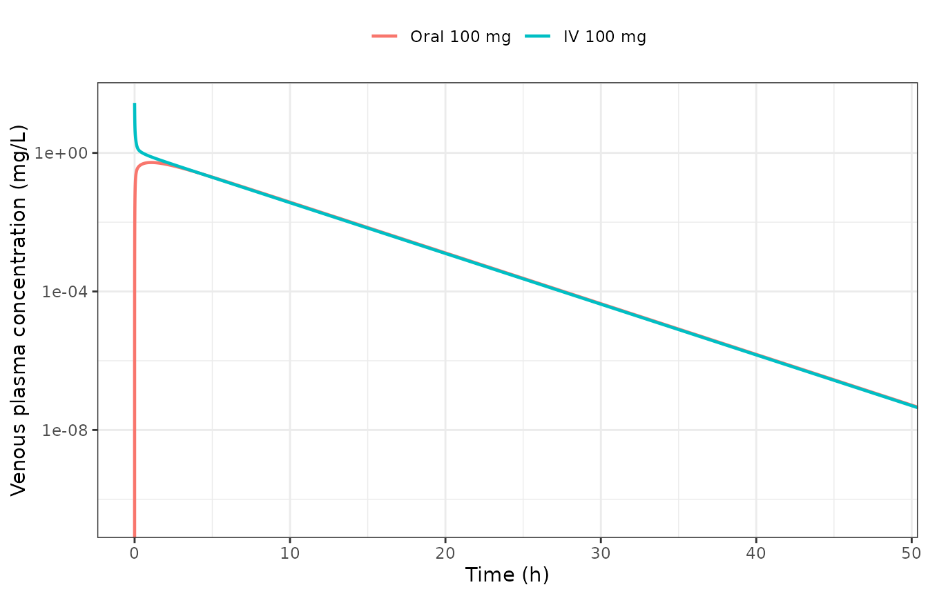
Venous plasma concentration after a 100 mg oral dose (the scenario the supplement initialises) and after a 100 mg intravenous bolus.
Because every partition coefficient is 1, the tissues are not merely similar at late times – they converge onto a single curve, which is the qualitative signature of the neutral template. The liver sits below the others because it is the eliminating organ, and the gut sits above during absorption because it receives the dose.
tissue_cols <- c("c_adipose", "c_brain", "c_muscle", "c_liver", "c_gut", "c_venous")
sim |>
  filter(treatment == "Oral 100 mg") |>
  select(time, all_of(tissue_cols)) |>
  pivot_longer(-time, names_to = "tissue", values_to = "conc") |>
  mutate(tissue = sub("^c_", "", tissue)) |>
  ggplot(aes(time, conc, colour = tissue)) +
  geom_line(linewidth = 0.7) +
  scale_y_log10() +
  coord_cartesian(xlim = c(0, 24)) +
  labs(x = "Time (h)", y = "Concentration (mg/L)", colour = NULL) +
  theme_bw()
#> Warning in scale_y_log10(): log-10 transformation introduced infinite values.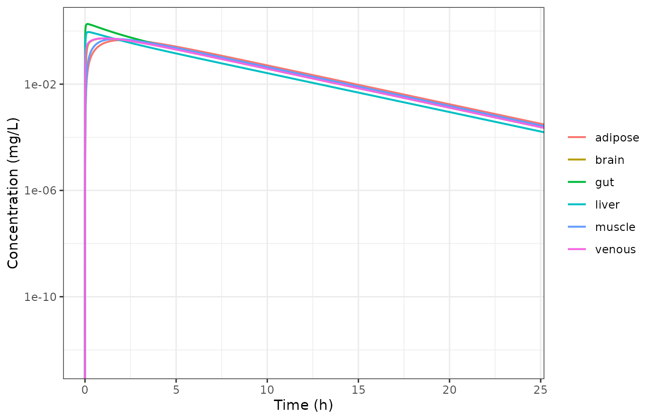
Tissue concentrations after the 100 mg oral dose. With every Kp set to 1 the non-eliminating tissues collapse onto the venous-blood curve once absorption is complete; liver (eliminating) and gut (dose entry) are the two exceptions.
Closed-form validation
With Kp = BP = fup = 1 and hepatic metabolism as the
only elimination route, integrating each compartment’s mass balance from
0 to infinity collapses the whole 16-state system to three exact
identities. They are worth deriving because they are independent of the
blood flows and volumes, so they test the clearance scaling and the
circulatory topology separately.
Total drug eliminated must equal the dose, and the only sink is
cl_met * cu_liver, so
AUC_liver = Dose / cl_met for either
route. Writing out the venous, lung and arterial balances then gives
AUC_arterial = AUC_venous, and substituting into the venous
balance yields:
-
Oral:
AUC(0-inf) = Dose / cl_met, henceCL/F = cl_metexactly. Blood flow cancels: complete absorption into the portal circulation means every absorbed molecule must clear the liver, whatever the perfusion. -
IV:
AUC(0-inf) = AUC_liver + Dose / Qh = Dose / CL_H, whereCL_H = Qh * cl_met / (Qh + cl_met)is the well-stirred hepatic clearance. -
Bioavailability:
F = AUC_oral / AUC_iv = Qh / (Qh + cl_met) = 1 - E_H.
The two arms also share one linear system, so they must share a terminal slope.
cl_h <- q_hepatic * cl_met / (q_hepatic + cl_met)
f_bioav <- q_hepatic / (q_hepatic + cl_met)

closed_form <- tibble::tibble(
  treatment  = c("Oral 100 mg", "IV 100 mg"),
  aucinf.obs = c(100 / cl_met, 100 / cl_h)
)
closed_form |> knitr::kable(digits = 6)| treatment | aucinf.obs |
|---|---|
| Oral 100 mg | 2.519526 |
| IV 100 mg | 3.710037 |
PKNCA validation
conc_data <- sim |>
  # Filter on missingness ONLY. Adding time > 0 or Cc > 0 would drop the
  # time-zero row that PKNCA needs to anchor AUC0-*.
  filter(!is.na(Cc)) |>
  select(id, treatment, time, Cc)

dose_data <- events |>
  filter(evid == 1L) |>
  transmute(
    id,
    treatment = ifelse(id == 1, "Oral 100 mg", "IV 100 mg"),
    time,
    amt,
    route = ifelse(id == 1, "extravascular", "intravascular")
  )

o_conc <- PKNCA::PKNCAconc(conc_data, Cc ~ time | id / treatment)
# PKNCAdose rejects slash grouping (unlike PKNCAconc); use `+` here.
o_dose <- PKNCA::PKNCAdose(dose_data, amt ~ time | id + treatment)
#> Found column named route, using it for the attribute of the same name.
o_data <- PKNCA::PKNCAdata(
  o_conc, o_dose,
  intervals = data.frame(
    start = 0, end = Inf,
    cmax = TRUE, tmax = TRUE, aucinf.obs = TRUE, half.life = TRUE, cl.obs = TRUE
  )
)
res <- PKNCA::pk.nca(o_data)

nca_wide <- as.data.frame(res) |>
  select(treatment, PPTESTCD, PPORRES) |>
  pivot_wider(names_from = PPTESTCD, values_from = PPORRES)
nca_wide |> knitr::kable(digits = 5)| treatment | cmax | tmax | tlast | clast.obs | lambda.z | r.squared | adj.r.squared | lambda.z.time.first | lambda.z.time.last | lambda.z.n.points | clast.pred | half.life | span.ratio | aucinf.obs | cl.obs |
|---|---|---|---|---|---|---|---|---|---|---|---|---|---|---|---|
| Oral 100 mg | 0.52870 | 1.075 | 72 | 0 | 0.33539 | 0.9999 | 0.9999 | 1.120 | 72 | 1637 | 0 | 2.06671 | 34.29608 | 2.51952 | 39.69004 |
| IV 100 mg | 27.79322 | 0.000 | 72 | 0 | 0.33819 | 0.9999 | 0.9999 | 0.165 | 72 | 1891 | 0 | 2.04959 | 35.04855 | 3.71006 | 26.95374 |
cmp <- nlmixr2lib::ncaComparisonTable(
  simulated     = nca_wide,
  reference     = closed_form,
  by            = "treatment",
  params        = "aucinf.obs",
  units         = c(aucinf.obs = "mg*h/L"),
  tolerance_pct = 20
)
knitr::kable(cmp)| NCA parameter | treatment | Reference | Simulated | % diff |
|---|---|---|---|---|
| AUC0-∞ (obs) (mg*h/L) | Oral 100 mg | 2.52 | 2.52 | -0.0% |
| AUC0-∞ (obs) (mg*h/L) | IV 100 mg | 3.71 | 3.71 | +0.0% |
The comparison table uses the standard 20% deviation flag, but the agreement here is far tighter than that, and the assertions below are set accordingly. Both sides of each comparison come from the same fixed parameter vector – there is no cohort and no sampled variability – so the only discrepancy is trapezoidal-integration error on a curve with a sharp absorption peak. A loose bound here would not be conservative, it would simply fail to test anything.
auc <- setNames(nca_wide$aucinf.obs, as.character(nca_wide$treatment))
thalf <- setNames(nca_wide$half.life, as.character(nca_wide$treatment))

checks <- tibble::tibble(
  check = c("oral AUCinf vs Dose/CLmet",
            "IV AUCinf vs Dose/CL_H",
            "F from AUC ratio vs Qh/(Qh+CLmet)"),
  simulated = c(auc[["Oral 100 mg"]], auc[["IV 100 mg"]],
                auc[["Oral 100 mg"]] / auc[["IV 100 mg"]]),
  expected  = c(100 / cl_met, 100 / cl_h, f_bioav)
) |>
  mutate(pct_diff = 100 * (simulated - expected) / expected)
knitr::kable(checks, digits = 8)| check | simulated | expected | pct_diff |
|---|---|---|---|
| oral AUCinf vs Dose/CLmet | 2.5195241 | 2.5195263 | -0.00008918 |
| IV AUCinf vs Dose/CL_H | 3.7100606 | 3.7100370 | 0.00063637 |
| F from AUC ratio vs Qh/(Qh+CLmet) | 0.6791059 | 0.6791108 | -0.00072554 |
stopifnot(
  # A deterministic solve against its own closed form: the only discrepancy is
  # trapezoidal error, which the refined grid drives to ~1e-3 %. The 0.05%
  # bound keeps ~50x headroom for solver/PKNCA version drift while still being
  # 400x tighter than the 20% table flag -- it would catch a single mistyped
  # digit anywhere in the clearance scaling or the circulatory topology.
  all(abs(checks$pct_diff) < 0.05),
  # CL/F must recover the scaled intrinsic clearance to the same precision.
  abs(nca_wide$cl.obs[nca_wide$treatment == "Oral 100 mg"] / cl_met - 1) < 5e-4,
  # Sanity on the well-stirred extraction: a moderate-clearance compound.
  f_bioav > 0.6, f_bioav < 0.75,
  # Both arms are the same 16-state linear system, so their TRUE terminal
  # slopes are identical. The residual difference is entirely lambda-z window
  # selection -- PKNCA starts the oral fit at ~1.1 h and the IV fit at ~0.2 h --
  # so this gets its own, looser bound than the exposure identities above.
  abs(thalf[["Oral 100 mg"]] / thalf[["IV 100 mg"]] - 1) < 0.02
)
# Independent of NCA: integrate the elimination flux and confirm the dose is
# conserved. Amount remaining is the sum of all 16 states.
ob <- sim |> filter(treatment == "IV 100 mg", !is.na(Cc)) |> arrange(time)
trap <- function(x, y) sum(diff(x) * (head(y, -1) + tail(y, -1)) / 2)
eliminated <- cl_met * unname(th[["fup"]]) * trap(ob$time, ob$c_liver)
remaining <- sum(ob[nrow(ob), mod$state])

tibble::tibble(
  quantity = c("eliminated by 72 h (mg)", "remaining in body at 72 h (mg)", "total (mg)"),
  value = c(eliminated, remaining, eliminated + remaining)
) |>
knitr::kable(digits = 4)| quantity | value |
|---|---|
| eliminated by 72 h (mg) | 100.0014 |
| remaining in body at 72 h (mg) | 0.0000 |
| total (mg) | 100.0014 |
Assumptions and deviations
-
The two main-text examples are not extracted.
Compound X (Table 1) and repaglinide (Table 3) are Simcyp runs whose
partition coefficients, absorption model and (for repaglinide)
permeability-limited liver geometry are not published. Their
physicochemical input tables and the observed-versus-predicted summary
in Table 2 are not sufficient to rebuild either model, and computing the
missing
Kpvectors ourselves from a tissue-composition method would be derivation rather than transcription. Only the deposited supplement model is extracted. - No IIV and no residual error. The source reports neither. Nothing is invented; the model is a deterministic typical-value simulation.
-
testesis a new canonical compartment. No previously registerednlmixr2libmodel resolved the gonads. It is added toinst/references/compartment-names.mdas a bare-organ compartment, withkp_testesadded to the partition-coefficient family ininst/references/parameter-names.md, following the precedent set byheart,skinandpancreas. Unlike the splanchnic organs, testes drains directly to venous blood, which is recorded in the register entry. -
Compound-specific parameters are on the linear scale, not
log-transformed.
checkModelConventions()suggestslkp_<organ>,lka,lfdepotandlcl_renal. That convention exists to keep estimation on an unbounded scale, and none of these parameters is estimated – all arefixed()template placeholders. The convention is also not representable here: the publishedcl_renalis exactly 0, andlog(0)is not finite. Keeping the linear scale additionally preserves verbatim transcription (Kpad = 1reads asfixed(1)), which is the point of a template file. Registry precedent:Han_2025_midazolam_pbpk.Rships the same warning class. -
fvol_plasma,fvol_erythrocytesand the two plasma volumes are carried but unused. The deposited code computesVpl,Vrb,Vplas_venandVplas_art; the perfusion-limited mass balance works in whole-blood volumes and never consumes them. They are retained for fidelity and are correctly excluded from the whole-body volume sum above.
Errata
-
Main-text Eq. 2 and the supplement code disagree on the free
concentration driving elimination. The narrative around Eq. 2
states that the rate of elimination is driven by the free concentration
in the venous blood leaving the tissue,
Cvu_T, whereCv_T = C_T / (Kp / BP); that would make the liver sinkC_liver * BP / Kp_liver * fup * CLmet. The deposited code instead writesCliverfree = Cliver*fup(and likewise for kidney), omitting theBP / Kpfactor. The two coincide exactly for the template as published, because it setsKp = BP = 1. They would diverge for any real compound. This file transcribes the deposited code, which is the runnable artifact and the thing the supplement offers for reuse; a user substituting a realKp_livershould be aware that Eq. 2 implies the extra factor. -
Table 2 prints the steady-state volume of distribution in
ml/min/kg. The row “Plasma V ss (ml/min/kg)” carries clearance units for a volume; the values (1.6 rat, 2.4 dog) are consistent withl/kg. This affects the compound X narrative only, not the extracted model.