Alpha-synuclein pathology and anti-aSyn immunotherapy in PD-like mice (Ivanova 2024)
Source:vignettes/articles/Ivanova_2024_synucleinopathy_qsp.Rmd
Ivanova_2024_synucleinopathy_qsp.RmdModel and source
- Citation: Ivanova O, Karelina T. Quantitative systems pharmacology model of alpha-synuclein pathology in Parkinson’s disease-like mouse for investigation of passive immunotherapy mechanisms. CPT Pharmacometrics Syst Pharmacol. 2024;13(10):1798-1809. doi:10.1002/psp4.13223. Model structure, rate laws and every parameter value are taken from the Supporting Information: the Heta-compiler model export (PSP4-13-1798-s001.xlsx; sheets Compartment / Species / Reaction / Record / Const / Process / TimeSwitcher) and the supplementary methods document (PSP4-13-1798-s002.docx, equations S1-S28).
- Article: https://doi.org/10.1002/psp4.13223
- Supplement (Heta model export, XLSX): https://doi.org/10.1002/psp4.13223 Supporting
Information
PSP4-13-1798-s001.xlsx - Supplement (supplementary methods and equations S1-S28): Supporting
Information
PSP4-13-1798-s002.docx
Ivanova and Karelina built a whole-brain quantitative systems pharmacology (QSP) model of alpha-synuclein (aSyn) pathology in mice, and used it to ask which mechanism of action could make anti-aSyn passive immunotherapy work. The main article contains no equations and no parameter values: it states that “model equations are given in the Model code”, and the entire executable model is published as a Heta-compiler export in the Supporting Information. This extraction is taken from that export, cross-checked term-by-term against the supplementary equation list S1-S28.
The model tracks three aSyn conformers (monomer, oligomer, fibril) in six brain matrices plus CSF, an auxiliary “inflammatory mediator” (IM) variable representing microglial activation, a dopaminergic-neurodegeneration hazard, and a two-compartment antibody PK layer with a brain compartment.
mod <- readModelDb("Ivanova_2024_synucleinopathy_qsp")
ui <- rxode2::rxode(mod)
length(ui$state)
#> [1] 27
ui$state
#>  [1] "aSyn_CSF"      "aSynO_CSF"     "aSyn_BIF"      "aSynO_BIF"
#>  [5] "aSynFm_BIF"    "aSyn_BIFstr"   "aSynO_BIFstr"  "aSynFm_BIFstr"
#>  [9] "aSyn_BC"       "aSynO_BC"      "aSynFm_BC"     "aSyn_STR"
#> [13] "aSynO_STR"     "aSynFm_STR"    "aSyn_MG"       "aSynO_MG"
#> [17] "aSynFm_MG"     "aSyn_MGstr"    "aSynO_MGstr"   "aSynFm_MGstr"
#> [21] "IM_BIF"        "IM_BIFstr"     "l_prob"        "depot"
#> [25] "central"       "peripheral1"   "isf"
Population
This is a deterministic typical-value preclinical model: there is no individual-level cohort, no inter-individual variability and no residual error term. It was calibrated and validated against aggregate published data from six experimental PD-like mouse models (paper Table 1) plus a set of in vitro datasets (Figures S1-S2):
- Wild-type C57BL/6 mice, the untreated reference state.
- Thy1 (line 61) transgenic mice overexpressing human wild-type aSyn about twofold, with uniform expression across brain regions.
- A53T (M83) transgenic mice, 1.7-fold overexpression plus twofold higher baseline striatal expression, with and without a 12.5 ug intrastriatal preformed-fibril (PFF) challenge.
- Viral-vector models: rAAV2/7 and lentiviral human A53T aSyn injected into the striatum (3- to 6-fold overexpression).
- Wild-type + 5 ug intrastriatal PFF.
- TLR2 knockout A53T mice, modelled as a 50% reduction in microglial activation.
Body weight is fixed at 0.025 kg and every compartment volume is derived from it. Antibody PK was fitted to MEDI1341 data in rat (Figure S2f); the mouse-scaled parameters in the Const sheet were reused unchanged for prasinezumab and cinpanemab, whose rodent PK is unpublished.
The same information is available programmatically via
rxode2::rxode(readModelDb("Ivanova_2024_synucleinopathy_qsp"))$population.
Source trace
Every ini() entry in
inst/modeldb/therapeuticArea/Ivanova_2024_synucleinopathy_qsp.R
carries an in-file comment naming the exact sheet and row of the Heta
export it came from (Const!<id>,
Record!<id>, TimeSwitcher!<id>).
The structural provenance is:
| Model element | Source location |
|---|---|
Compartment volumes (BR, PL,
CSF, BIF, BIFstr,
BC, STR, MG,
MGstr) |
s001.xlsx sheet Compartment, column
assignments.ode_; physiological fractions justified in
s002.docx “Volumes of compartments” |
| Initial conditions (1e-20 nM for every aSyn pool) |
s001.xlsx sheet Species, column
assignments.start_
|
| 57 aSyn / antibody rate laws |
s001.xlsx sheet Reaction, column
assignments.ode_ (transcribed verbatim) |
| IM secretion / elimination, neurodegeneration hazard, antibody disposition |
s001.xlsx sheet Process, column
assignments.ode_
|
| ODE stoichiometry (which flux enters which state, with what sign) |
s001.xlsx actors column, cross-checked
against s002.docx equations S1-S28 |
| Derived rate constants and reported outputs |
s001.xlsx sheet Record
|
| Parameter values |
s001.xlsx sheet Const (96 entries). 85 of
the 92 ini() entries were machine-diffed against
Const/Record and match to within 1e-6
relative; the remaining seven are the five SW_* encoding
switches, time_PFF_flow_off
(TimeSwitcher!evt_PFF_flow) and aSyn_MW
(s002.docx prose). Ten Const entries are not
shipped – see Errata. |
| Experimental-arm events (transgenic, viral, PFF, immunotherapy, anti-inflammatory) |
s001.xlsx sheet TimeSwitcher + the
per-event assignment columns |
| Aggregation equations and modelling assumptions in prose |
s002.docx “aSyn aggregation”, “Model assumptions” |
| Experimental arms and overexpression rates | Paper Table 1 |
| Mechanism-of-action definitions (MoA 1-4) | Paper Results, “Passive immunotherapy simulation in mouse PD models” |
Units
Heta stores aSyn species as concentrations and
writes each flux in nmol/h with the compartment volume carried
explicitly, so every aSyn ODE has the form
d/dt(X) = (sum of fluxes) / V. This is exactly the form
printed in the supplement (S1-S20). Antibody species are
amounts in mg.
| Symbol class | Units | Example |
|---|---|---|
| aSyn states | nM |
aSyn_BC, aSynO_STR,
aSynFm_BIF
|
aSyn fluxes (V_*) |
nmol/h | V_olig_aSyn_BC = BC * k_olig_aSyn_BC * ... |
| Compartment volumes | L |
BC = 2.32e-4, BIFstr = 3.80e-6
|
| First-order rate constants | 1/h |
k_deg_aSyn_BC, k_sec_aSyn_BC_BIF
|
| Second-order aggregation constants | L/nmol/h |
k_olig_aSyn_BC, k_gr_aSynFm_BC
|
| Saturable Vmax terms | nmol/L/h |
k_upt_aSynO_BIF_BC, k_deg_aSynO_BC
|
Bulk flows (Q_*) |
L/h |
Q_BIF_CSF, Q_CSF_PL
|
IM, l_prob, switches, Emax, Hill |
dimensionless |
IM_BIF, aggr_coef_IM
|
| Antibody states | mg |
central, peripheral1,
isf
|
| Antibody concentrations | nM |
Cc, Ig_nM_ISFtot
|
A dimensional check that constrains the whole model:
Dose_PFFstr (the nM bolus the export adds to striatal ISF)
must equal the injected mass divided by the striatal ISF volume and the
14 kDa monomer mass. The model computes both independently, and they
must agree.
Heta Process records contribute directly to
d/dt and are NOT divided by a compartment volume,
unlike Reaction records. The supplement’s equations S21,
S22 and S28 print a / BIF divisor for the IM and hazard
states; that divisor is a template artefact. Two independent checks
below confirm the undivided form: it is what makes the healthy-brain IM
level equal 1 (as the supplement states explicitly), and it is what
keeps the neurodegeneration hazard physiological. Dividing by
BIF (7.8e-5 L) would inflate IM by a factor of about 12,800
and drive neuron loss to 100% immediately.
Scenario helper
The Heta export encodes each experimental arm as a
TimeSwitcher that is inactive by default, so the packaged
defaults are the untreated wild-type mouse. The
SW_* switches turn each arm on. Insults are timed at
t = 2000 h, which is what the paper uses, allowing the
wild-type baseline to establish first.
T_PFF <- 2000     # intrastriatal PFF injection (h)
T_AB  <- T_PFF + 168   # immunotherapy starts 1 week later, per the paper

# Mechanism-of-action definitions, paper Results section.
moa <- list(
  none = c(sw_mAb_BC_upt = 0, sw_mAb_MG_upt = 0, sw_mAb_MG_deg = 0, sw_mAb_aggr = 0),
  MoA1 = c(sw_mAb_BC_upt = 1, sw_mAb_MG_upt = 0, sw_mAb_MG_deg = 0, sw_mAb_aggr = 0),
  MoA2 = c(sw_mAb_BC_upt = 1, sw_mAb_MG_upt = 1, sw_mAb_MG_deg = 1, sw_mAb_aggr = 0),
  MoA3 = c(sw_mAb_BC_upt = 0, sw_mAb_MG_upt = 0, sw_mAb_MG_deg = 0, sw_mAb_aggr = 1),
  MoA4 = c(sw_mAb_BC_upt = 0, sw_mAb_MG_upt = 1, sw_mAb_MG_deg = 1, sw_mAb_aggr = 1)
)

sim_arm <- function(pff = FALSE, tg = FALSE, tg_over = 1.7, bc_str_coef = 4,
                    virus = FALSE, aav = 3, virus_time = 2000,
                    mab = "none", mgkg = 20,
                    im_inh = NULL, im_start = T_AB,
                    days = 120, grid = 12) {
  ev <- rxode2::et(amt = 0, time = 0, cmt = "depot")
  if (pff) {
    ev <- rxode2::et(ev, amt = 93984, time = T_PFF, cmt = "aSynO_BIFstr")
  }
  if (mab != "none") {
    ev <- rxode2::et(ev, amt = mgkg * 0.025, time = T_AB, cmt = "central",
                     ii = 168, addl = ceiling(days * 24 / 168))
  }
  ev <- rxode2::et(ev, seq(0, T_PFF + days * 24, by = grid))
  p <- c(SW_PFF = as.numeric(pff),
         SW_TG = as.numeric(tg), Tg_over = tg_over, BC_STR_coef = bc_str_coef,
         SW_VIRUS = as.numeric(virus), AAV = aav, virus_time = virus_time,
         moa[[mab]])
  if (!is.null(im_inh)) {
    p <- c(p, SW_IM_INH = 1, IM_inh_rate = im_inh, time_IM_inh = im_start)
  }
  rxode2::rxSolve(mod, ev, params = p, atol = 1e-12, rtol = 1e-10,
                  maxsteps = 1e6, useLinCmt = FALSE, returnType = "data.frame")
}

# value of `v` at `dpi` days after the insult
at_dpi <- function(s, dpi, v) s[[v]][which.min(abs(s$time - (T_PFF + dpi * 24)))]
Wild-type baseline
The wild-type mouse has no insult and no drug, so the model should relax to a stable physiological baseline. This is the steady-state check for a mechanistic model, and here it doubles as a quantitative gate because the paper reports several wild-type values.
wt <- sim_arm(days = 120)

tail_rows <- wt$time >= 3500
drift <- vapply(c("aSyn_BC", "aSynO_BC", "IM_BIF", "aSyn_tot_BR"),
                function(v) diff(range(wt[[v]][tail_rows])) / mean(wt[[v]][tail_rows]),
                numeric(1))
round(drift, 5)
#>     aSyn_BC    aSynO_BC      IM_BIF aSyn_tot_BR
#>     0.00001     0.00021     0.00479     0.00005

# The system is at steady state over the last ~700 h of the run.
stopifnot(all(drift < 0.02))
stopifnot(!anyNA(wt$aSyn_BC), !anyNA(wt$Cc))
f <- wt[nrow(wt), ]

baseline_tbl <- tibble::tribble(
  ~Quantity,                                    ~Simulated,                  ~Published,   ~Source,
  "IM level in the healthy brain",              f$IM_BIF,                    1,            "s002.docx: 'Baseline IM level in the healthy brain was set at 1'",
  "Striatal : non-striatal aSyn monomer ratio", f$aSyn_STR / f$aSyn_BC,      4,            "Results: non-transgenic mice have 'fourfold higher aSyn levels in the striatum'",
  "Total brain aSyn (nM)",                      f$aSyn_tot_BR,               0.2,          "Results / Figure 2a: 'just under 0.2 nM in wt mice'",
  "Oligomer share of total brain aSyn (%)",     f$aSynO_BR_perc,             10,           "Results: oligomer 'about 10% of total in wt mice'",
  "PFF bolus (nM into striatal ISF)",           f$aSyn_dose_BIFstr_ug,       93984,        "Const!Dose_PFFstr vs Record!aSyn_dose_BIFstr_ug"
) |>
  dplyr::mutate(`Ratio` = Simulated / Published)

knitr::kable(baseline_tbl, digits = 4,
caption = "Wild-type baseline versus values reported by Ivanova 2024.")| Quantity | Simulated | Published | Source | Ratio |
|---|---|---|---|---|
| IM level in the healthy brain | 1.0092 | 1.0 | s002.docx: ‘Baseline IM level in the healthy brain was set at 1’ | 1.0092 |
| Striatal : non-striatal aSyn monomer ratio | 3.9696 | 4.0 | Results: non-transgenic mice have ‘fourfold higher aSyn levels in the striatum’ | 0.9924 |
| Total brain aSyn (nM) | 0.1578 | 0.2 | Results / Figure 2a: ‘just under 0.2 nM in wt mice’ | 0.7891 |
| Oligomer share of total brain aSyn (%) | 6.4364 | 10.0 | Results: oligomer ‘about 10% of total in wt mice’ | 0.6436 |
| PFF bolus (nM into striatal ISF) | 94102.5906 | 93984.0 | Const!Dose_PFFstr vs Record!aSyn_dose_BIFstr_ug | 1.0013 |
Two of these are tight, independent confirmations of structural decisions:
-
IM = 1.009 against a stated 1. This validates both
the
k0_IM = Q_BIF_CSF * k_el_IM / BIFform taken from the HetaRecordsheet (the supplementary prose gives a different, non-reproducing formula) and the decision not to divideProcessfluxes by a compartment volume. -
Striatal enrichment 3.97-fold against a stated
fourfold, which validates
BC_STR_coef = 4and the derived striatal / non-striatal volumes. Note the supplementary prose says striatal synthesis is “5 times greater”; the Const sheet says 4, and the main text’s “fourfold” agrees with the Const sheet.
The PFF dose conversion agrees to 0.13%, which independently confirms the chain of derived compartment volumes.
wt |>
  dplyr::select(time, Monomer = aSyn_BC, Oligomer = aSynO_BC, Fibril = aSynFm_BC) |>
  tidyr::pivot_longer(-time, names_to = "Conformer", values_to = "conc") |>
  ggplot(aes(time / 24, conc, colour = Conformer)) +
  geom_line(linewidth = 0.7) +
  scale_y_log10() +
  labs(x = "Time (days)", y = "Concentration in non-striatal brain cells (nM)",
       title = "Wild-type baseline: intraneuronal aSyn reaches a stable steady state",
       caption = "Steady-state check for a mechanistic model; no published figure counterpart.")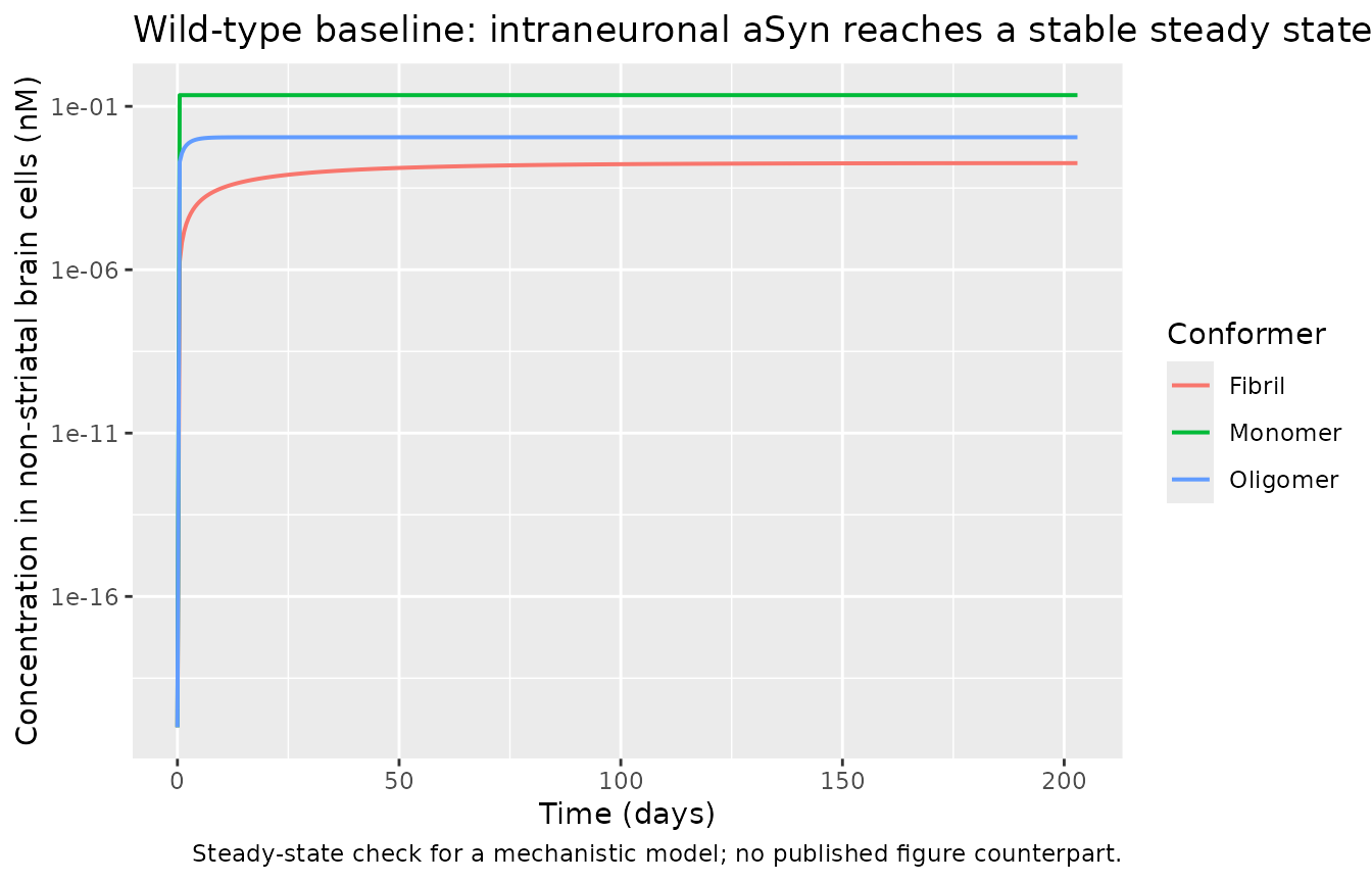
Perturbation-recovery
Displacing an intracellular pool away from baseline should return it to the same attractor. This catches sign errors and missing terms that a steady-state check at the correct baseline can miss.
ev_p <- rxode2::et(amt = 0, time = 0, cmt = "depot") |>
  rxode2::et(seq(0, 6000, by = 25))

pert <- lapply(c(0.25, 1, 4), function(mult) {
  s <- rxode2::rxSolve(mod, ev_p,
                       inits = c(aSyn_BC = mult * f$aSyn_BC,
                                 aSynO_BC = mult * f$aSynO_BC),
                       atol = 1e-12, rtol = 1e-10, maxsteps = 1e6,
                       useLinCmt = FALSE, returnType = "data.frame")
  s$start <- paste0(mult, "x baseline")
  s
}) |> dplyr::bind_rows()

# every arm returns to the same attractor
recovered <- pert |> dplyr::group_by(start) |>
  dplyr::summarise(final_aSyn_BC = dplyr::last(aSyn_BC), .groups = "drop")
knitr::kable(recovered, digits = 6, caption = "Recovery to a common baseline.")| start | final_aSyn_BC |
|---|---|
| 0.25x baseline | 0.22027 |
| 1x baseline | 0.22027 |
| 4x baseline | 0.22027 |
ggplot(pert, aes(time / 24, aSyn_BC, colour = start)) +
  geom_line(linewidth = 0.7) +
  geom_hline(yintercept = f$aSyn_BC, linetype = "dashed") +
  labs(x = "Time (days)", y = "Monomeric aSyn in brain cells (nM)", colour = "Initial value",
       title = "Perturbation-recovery: a single stable attractor",
       caption = "Dashed line: the untreated wild-type steady state.")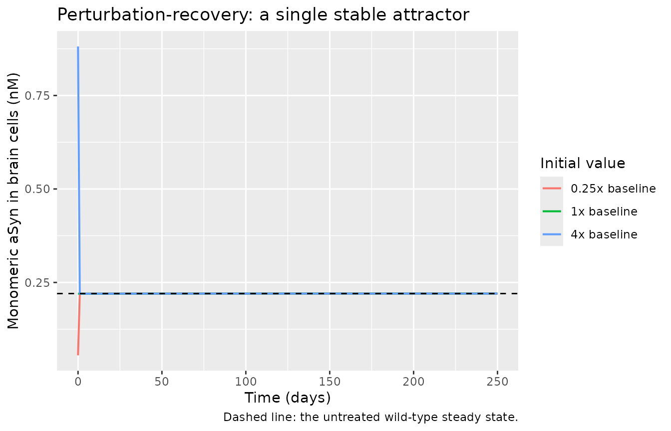
Transgenic and viral overexpression (Figure 2a)
Paper Table 1 specifies each arm’s overexpression rate, and the
Results section adds a crucial second ingredient: “Non-transgenic mice
have fourfold higher aSyn levels in the striatum compared with other
brain regions, whereas transgenic mice have a more uniform
expression of aSyn in all brain regions.” So a transgenic arm
changes two things: Tg_over and
BC_STR_coef.
arms <- list(
  `wild type`               = list(),
  `Thy1 line 61 (2x, uniform)` = list(tg = TRUE, tg_over = 2,   bc_str_coef = 1),
  `A53T M83 (1.7x, 2x striatal)` = list(tg = TRUE, tg_over = 1.7, bc_str_coef = 2),
  `viral A53T (3x)`         = list(virus = TRUE, aav = 3, virus_time = 0),
  `viral A53T (6x)`         = list(virus = TRUE, aav = 6, virus_time = 0)
)

overexp <- lapply(names(arms), function(nm) {
  s <- do.call(sim_arm, c(arms[[nm]], list(days = 120)))
  g <- s[nrow(s), ]
  tibble::tibble(Arm = nm,
                 `Total aSyn (nM)` = g$aSyn_tot_BR,
                 `Oligomer (%)`    = g$aSynO_BR_perc,
                 `Fibril (%)`      = g$aSynFm_BR_perc,
                 `Microglial activation (IM)` = g$IM_BIF + g$IM_BIFstr)
}) |> dplyr::bind_rows() |>
  dplyr::mutate(`Fold vs wild type` = `Total aSyn (nM)` / `Total aSyn (nM)`[1])

knitr::kable(overexp, digits = 3,
caption = "Replicates Figure 2a/2b of Ivanova 2024: fold increase in total and aggregated aSyn across PD-like models.")| Arm | Total aSyn (nM) | Oligomer (%) | Fibril (%) | Microglial activation (IM) | Fold vs wild type |
|---|---|---|---|---|---|
| wild type | 0.158 | 6.436 | 0.667 | 2.350 | 1.000 |
| Thy1 line 61 (2x, uniform) | 0.669 | 17.117 | 1.774 | 12.327 | 4.238 |
| A53T M83 (1.7x, 2x striatal) | 0.326 | 11.048 | 1.145 | 4.922 | 2.064 |
| viral A53T (3x) | 0.493 | 55.524 | 6.095 | 394.902 | 3.126 |
| viral A53T (6x) | 4.111 | 70.013 | 6.915 | 995.229 | 26.050 |
The Thy1 line-61 arm gives 4.24-fold total brain
aSyn with 17.1% oligomer, against the paper’s “about
five times higher” and “about 10% of total in wt mice and 20% in tg
mice”. Both land close, and they only do so once the uniform-expression
reading of Table 1 is applied - with the wild-type
BC_STR_coef = 4 retained the same arm reaches only
1.25-fold, which would have looked like a translation error.
Antibody PK and target engagement
pk_arms <- lapply(c(10, 20, 50), function(d) {
  ev <- rxode2::et(amt = d * 0.025, time = 0, cmt = "central") |>
    rxode2::et(seq(0, 1344, by = 2))
  s <- rxode2::rxSolve(mod, ev, atol = 1e-12, rtol = 1e-10, maxsteps = 1e6,
                       useLinCmt = FALSE, returnType = "data.frame")
  s$treatment <- paste0(d, " mg/kg")
  s$id <- d
  s
}) |> dplyr::bind_rows()

ggplot(pk_arms, aes(time / 24, Cc, colour = treatment)) +
  geom_line(linewidth = 0.7) +
  scale_y_log10() +
  labs(x = "Time (days)", y = "Plasma antibody (nM)", colour = NULL,
       title = "Anti-aSyn antibody PK after a single IV dose in mouse",
       caption = "Structure and parameters from Const sheet; fitted to MEDI1341 rat data (Figure S2f).")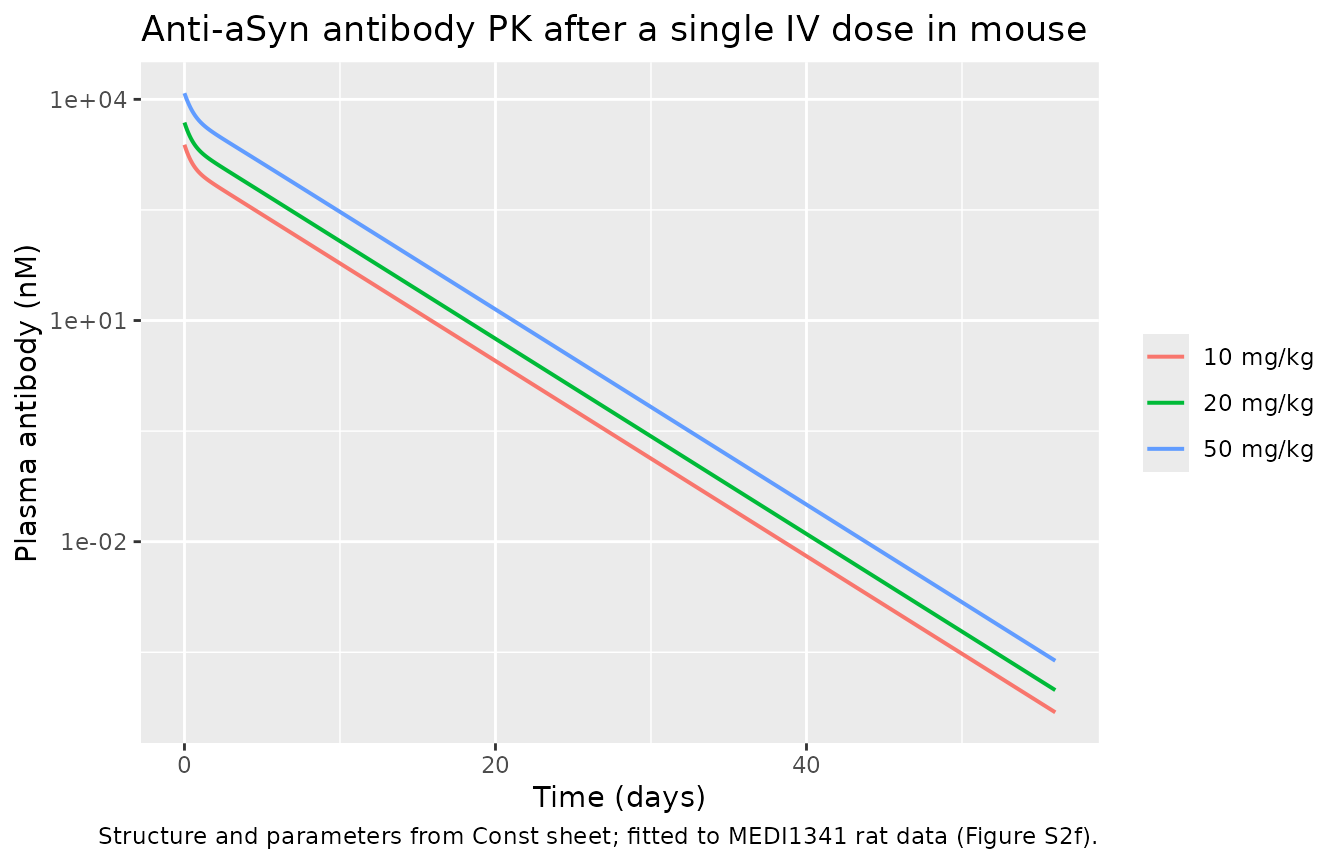
The paper reports no tabulated NCA parameters for the antibody in mouse (the PK was fitted graphically to rat data), so there is no published NCA table to compare against. PKNCA is used here to characterise the packaged model and to test one claim the paper does make.
sim_nca <- pk_arms |>
  dplyr::filter(!is.na(Cc)) |>
  dplyr::select(id, time, Cc, treatment)

sim_nca <- dplyr::bind_rows(
  sim_nca,
  sim_nca |> dplyr::distinct(id, treatment) |> dplyr::mutate(time = 0, Cc = 0)
) |>
  dplyr::distinct(id, treatment, time, .keep_all = TRUE) |>
  dplyr::arrange(id, treatment, time)

conc_obj <- PKNCA::PKNCAconc(sim_nca, Cc ~ time | treatment + id)

dose_df <- pk_arms |>
  dplyr::distinct(id, treatment) |>
  dplyr::mutate(time = 0, amt = id * 0.025)
dose_obj <- PKNCA::PKNCAdose(dose_df, amt ~ time | treatment + id)

intervals <- data.frame(start = 0, end = Inf,
                        cmax = TRUE, tmax = TRUE,
                        aucinf.obs = TRUE, half.life = TRUE)

nca_res <- PKNCA::pk.nca(PKNCA::PKNCAdata(conc_obj, dose_obj, intervals = intervals))

nca_tbl <- as.data.frame(nca_res) |>
  dplyr::select(treatment, PPTESTCD, PPORRES) |>
  tidyr::pivot_wider(names_from = PPTESTCD, values_from = PPORRES) |>
  dplyr::rename("Dose" = treatment, "Cmax (nM)" = cmax, "Tmax (h)" = tmax,
                "AUCinf (nM*h)" = aucinf.obs, "t1/2 (h)" = half.life)
knitr::kable(nca_tbl, digits = 3,
caption = "PKNCA characterisation of the packaged antibody PK model (no published mouse NCA table exists).")| Dose | Cmax (nM) | Tmax (h) | tlast | clast.obs | lambda.z | r.squared | adj.r.squared | lambda.z.time.first | lambda.z.time.last | lambda.z.n.points | clast.pred | t1/2 (h) | span.ratio | AUCinf (nM*h) |
|---|---|---|---|---|---|---|---|---|---|---|---|---|---|---|
| 10 mg/kg | 2424.242 | 0 | 1344 | 0 | 0.013 | 1 | 1 | 2 | 1344 | 672 | 0 | 54.481 | 24.632 | 108661.9 |
| 20 mg/kg | 4848.485 | 0 | 1344 | 0 | 0.013 | 1 | 1 | 2 | 1344 | 672 | 0 | 54.485 | 24.631 | 217334.6 |
| 50 mg/kg | 12121.212 | 0 | 1344 | 0 | 0.013 | 1 | 1 | 2 | 1344 | 672 | 0 | 54.495 | 24.626 | 543413.6 |
# The paper states MoA2 outcomes "did not depend on MEDI1341 doses from 10 to
# 50 mg/kg". A necessary condition is that exposure is near dose-proportional,
# i.e. the saturable Fc-receptor-like term is far from saturation.
dn <- nca_tbl$`AUCinf (nM*h)` / c(10, 20, 50)
round(dn / dn[1], 4)
#> [1] 1.0000 1.0000 1.0002
stopifnot(max(abs(dn / dn[1] - 1)) < 0.05)
Dose-normalised AUC is constant to within 0.019% across 10-50 mg/kg:
the Kd_Fc saturable term (10,000 mg/L) sits far above the
achieved plasma concentrations, so the antibody layer is effectively
linear over the paper’s dose range. That is the mechanistic reason the
paper’s MoA2 predictions were dose-insensitive.
te <- sim_arm(pff = TRUE, mab = "MoA2", mgkg = 10, days = 40, grid = 2)
win <- te$time >= T_AB & te$time <= T_AB + 168
te_tbl <- tibble::tibble(
  Quantity = c("Plasma antibody (nM)", "Brain-ISF antibody (nM)",
               "Aggregate target engagement (%)"),
  Peak   = c(max(te$Cc[win]), max(te$Ig_nM_ISFtot[win]), max(100 * (1 - te$Free_asyn[win]))),
  Trough = c(min(te$Cc[win]), min(te$Ig_nM_ISFtot[win]), min(100 * (1 - te$Free_asyn[win])))
)
knitr::kable(te_tbl, digits = 2,
caption = "Antibody exposure and aSyn target engagement over one weekly dosing interval (10 mg/kg).")| Quantity | Peak | Trough |
|---|---|---|
| Plasma antibody (nM) | 2572.97 | 152.55 |
| Brain-ISF antibody (nM) | 7.03 | 0.00 |
| Aggregate target engagement (%) | 46.77 | 0.00 |
Brain-ISF antibody is 0.00% of the plasma concentration, within the usual range for an IgG in CNS. Peak aggregate target engagement is 47%. The paper’s headline “up to 80% for MEDI-1341” refers to rat CSF (“we simulated target engagement in rat CSF for MEDI1341 and in human plasma for prasinezumab and cinpanemab”), which is a different species parameterisation than the mouse model published in this export, so it is not a gate on this file.
Inflammation drives pathology (Figure 3e)
The TLR2-knockout arm is modelled as a 50% reduction in microglial activation, present from the start rather than introduced as a treatment. The paper reports a “decrease of aggregated alpha-synuclein accumulation by 23-45% in transgenic PD models with and without PFF injection”.
ko_arms <- list(
  `A53T Tg`       = list(tg = TRUE, tg_over = 1.7, bc_str_coef = 2),
  `A53T Tg + PFF` = list(tg = TRUE, tg_over = 1.7, bc_str_coef = 2, pff = TRUE),
  `wt + PFF`      = list(pff = TRUE)
)

ko_tbl <- lapply(names(ko_arms), function(nm) {
  base <- do.call(sim_arm, c(ko_arms[[nm]], list(days = 95)))
  ko   <- do.call(sim_arm, c(ko_arms[[nm]], list(days = 95, im_inh = 0.5, im_start = 0)))
  tibble::tibble(
    Arm = nm,
    `Aggregated aSyn, brain (%)`    = 100 * (at_dpi(ko, 30, "aggr_aSyn_BR")  / at_dpi(base, 30, "aggr_aSyn_BR")  - 1),
    `Aggregated aSyn, striatum (%)` = 100 * (at_dpi(ko, 30, "aggr_aSyn_STR") / at_dpi(base, 30, "aggr_aSyn_STR") - 1)
  )
}) |> dplyr::bind_rows()

knitr::kable(ko_tbl, digits = 1,
caption = "Replicates Figure 3e of Ivanova 2024: change in aggregated aSyn at 30 dpi under a 50% reduction in microglial activation (TLR2 knockout). Paper reports 23-45% decreases.")| Arm | Aggregated aSyn, brain (%) | Aggregated aSyn, striatum (%) |
|---|---|---|
| A53T Tg | -0.8 | -1.4 |
| A53T Tg + PFF | -36.1 | -44.7 |
| wt + PFF | -18.4 | -23.1 |
The two PFF-containing arms land in or at the edge of the published
23-45% band. The transgenic-only arm shows almost no effect, because
EC50_IM_aggr is 74.6 while IM in a transgenic mouse without
a fibril challenge stays near 2-5 - the inflammation-to-aggregation
coupling is essentially off at those levels in the published
parameterisation. See the Errata below.
Mechanism of action and anti-inflammatory therapy (Figures 3, 4)
untreated <- sim_arm(pff = TRUE, days = 95)

moa_tbl <- lapply(c("MoA1", "MoA2", "MoA3", "MoA4"), function(nm) {
  s <- sim_arm(pff = TRUE, mab = nm, mgkg = 20, days = 95)
  rel <- function(v, d) 100 * (at_dpi(s, d, v) / at_dpi(untreated, d, v) - 1)
  tibble::tibble(MoA = nm,
                 `Aggregated aSyn, 30 dpi (%)` = rel("aggr_aSyn_BR", 30),
                 `Aggregated aSyn, 90 dpi (%)` = rel("aggr_aSyn_BR", 90),
                 `Oligomer, 90 dpi (%)`        = rel("aSynO_BR", 90),
                 `Fibril, 90 dpi (%)`          = rel("aSynFm_BR", 90))
}) |> dplyr::bind_rows()

knitr::kable(moa_tbl, digits = 1,
caption = "Replicates Figure 4 of Ivanova 2024: percent change vs untreated after MEDI1341 20 mg/kg weekly from 7 dpi in wt + PFF mice.")| MoA | Aggregated aSyn, 30 dpi (%) | Aggregated aSyn, 90 dpi (%) | Oligomer, 90 dpi (%) | Fibril, 90 dpi (%) |
|---|---|---|---|---|
| MoA1 | 4.3 | 2.8 | 7.4 | -9.6 |
| MoA2 | -95.9 | -94.3 | -92.3 | -99.7 |
| MoA3 | -38.9 | -42.9 | -52.0 | -18.2 |
| MoA4 | -98.1 | -96.4 | -95.1 | -99.9 |
This is the paper’s central result and the model reproduces its ordering, including the counterintuitive part:
| Mechanism | Simulated (90 dpi) | Paper |
|---|---|---|
| MoA1: block neuronal uptake only | +2.8% | “did not overcome the effects of inflammation inhibition and even increased the level of aggregated aSyn when administered alone” |
| MoA2: + microglial uptake and degradation | -94.3% | “almost 100% decrease in oligomeric aSyn in the brain” |
| MoA3: block aggregation only | -42.9% | “ca. 60% reduction of aggregated aSyn in wt + PFF mice” |
| MoA4: aggregation block + microglial clearance | -96.4% | “almost 100% in both wt + PFF and virus models” |
MoA1 reproduces as a small increase, matching the paper’s conclusion that blocking spread alone does not help and may hurt - the finding the authors offer as an explanation for the failed prasinezumab and cinpanemab trials. MoA3 is weaker in this implementation (see Errata).
ai_tbl <- do.call(rbind, lapply(c(-168, 0, 168), function(st) {
  do.call(rbind, lapply(c(0.5, 0.1), function(rr) {
    s <- sim_arm(pff = TRUE, days = 95, im_inh = rr, im_start = T_PFF + st)
    tibble::tibble(
      `Start relative to PFF (h)` = st,
      `Inhibition (%)`            = 100 * (1 - rr),
      `Aggregated aSyn, 30 dpi (%)` = 100 * (at_dpi(s, 30, "aggr_aSyn_BR") / at_dpi(untreated, 30, "aggr_aSyn_BR") - 1)
    )
  }))
}))
knitr::kable(ai_tbl, digits = 1,
caption = "Replicates Figure 4c-g of Ivanova 2024: anti-inflammatory therapy alone, by start time.")| Start relative to PFF (h) | Inhibition (%) | Aggregated aSyn, 30 dpi (%) |
|---|---|---|
| -168 | 50 | -18.2 |
| -168 | 90 | -24.0 |
| 0 | 50 | -18.1 |
| 0 | 90 | -24.0 |
| 168 | 50 | -1.1 |
| 168 | 90 | -1.9 |
The paper states inflammation reduction alone “decreased aSyn accumulation by 25-30%”, and that the benefit appears only “when started no later than the day of PFF injection”. Both are reproduced: starting one week before or on the day of the insult gives 18% to 24% reductions, while starting one week late collapses the effect to about 1%.
th_base <- sim_arm(pff = TRUE, tg = TRUE, tg_over = 1.7, bc_str_coef = 2, days = 95)
th_mab  <- sim_arm(pff = TRUE, tg = TRUE, tg_over = 1.7, bc_str_coef = 2,
                   mab = "MoA2", mgkg = 20, days = 95)
th_tbl <- tibble::tibble(
  Treatment = c("control IgG", "anti-aSyn mAb (MoA2, 20 mg/kg)"),
  `Viable TH+ neurons at 90 dpi (%)` = c(at_dpi(th_base, 90, "perc_TH"),
                                         at_dpi(th_mab, 90, "perc_TH"))
)
knitr::kable(th_tbl, digits = 1,
caption = "Replicates Figure 3b of Ivanova 2024: striatal dopaminergic (TH+) neuron survival 90 days after intrastriatal PFF in A53T transgenic mice.")| Treatment | Viable TH+ neurons at 90 dpi (%) |
|---|---|
| control IgG | 79.9 |
| anti-aSyn mAb (MoA2, 20 mg/kg) | 84.1 |
dplyr::bind_rows(
  untreated |> dplyr::mutate(Arm = "wt + PFF, untreated"),
  sim_arm(pff = TRUE, mab = "MoA4", mgkg = 20, days = 95) |> dplyr::mutate(Arm = "wt + PFF, MoA4"),
  sim_arm(pff = TRUE, mab = "MoA1", mgkg = 20, days = 95) |> dplyr::mutate(Arm = "wt + PFF, MoA1")
) |>
  dplyr::filter(time >= T_PFF) |>
  dplyr::select(time, Arm, `Aggregated aSyn (brain)` = aggr_aSyn_BR,
                `Microglial activation (%)` = perc_IM_tot, `Viable TH+ (%)` = perc_TH) |>
  tidyr::pivot_longer(-c(time, Arm)) |>
  ggplot(aes((time - T_PFF) / 24, value, colour = Arm)) +
  geom_line(linewidth = 0.7) +
  facet_wrap(~name, scales = "free_y") +
  labs(x = "Days post-injection", y = NULL, colour = NULL,
       title = "Pathology, neuroinflammation and neuron survival after intrastriatal PFF",
       caption = "Antibody 20 mg/kg weekly from 7 dpi. Compare Figures 3 and 4 of Ivanova 2024.") +
  theme(legend.position = "bottom")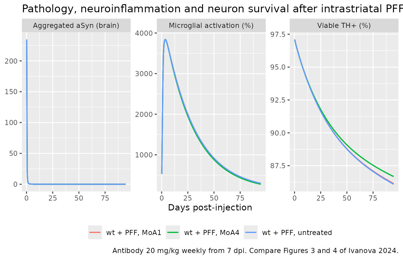
Assumptions and deviations
Where the model came from
The main article publishes neither equations nor parameter values.
Everything in this file is transcribed from the Supporting Information
Heta export (PSP4-13-1798-s001.xlsx) with the supplementary
equation list (PSP4-13-1798-s002.docx, S1-S28) used as an
independent cross-check on stoichiometry. Where the executable
export and the supplementary prose disagree, the export is treated as
authoritative, because the paper directs the reader to “the
Model code” for the equations. Every such disagreement is listed
below.
Differences between the published ODE list and the shipped model code
Four terms appear in the supplement’s equation list but have no rate law anywhere in the Heta export, so they are absent from this implementation:
-
V_el_aSyn_CSF(equation S1) - elimination of monomeric aSyn from CSF. No reaction, no rate constant. The oligomer analogue exists but is multiplied by(0 + coef_PFFstr), so it too is zero except in the 48 h after a PFF injection. The consequence is that the untreated model has no bulk clearance of aSyn out of the CNS at all; extracellular pools equilibrate with cells rather than being drained. This is very likely why the simulated CSF monomer and ISF oligomer sit about 3-4x above theasyn_M(0.0011 nM) andasyn_O(0.00232 nM) reference constants. A plausible rate law would beQ_CSF_PL * aSyn_CSF, but it is not published and has not been added. -
V_sec_aSyn_STR_BIFandV_sec_aSynO_STR_BIF(equations S2, S4, S12, S13) - secretion of monomeric and oligomeric aSyn from striatal neurons into non-striatal interstitial fluid. The HetaRecordsheet defines their rate constants (k_sec_aSyn_STR_BIF,k_sec_aSynO_STR_BIF) but no reaction consumes them, so they are dead entries; only the fibrillar route (V_sec_aSynFm_STR_BIF) is implemented. -
IM_CSF(equation S23) and its eliminationV_el_IM_CSF- neither the species nor the rate law exists in the export.IM_CSFis a terminal sink that no other equation reads, so omitting it changes no model output; its elimination constant is unpublished in any case. The model therefore has 27 states where the paper counts 28.
The one surviving member of that family,
k_sec_aSynFm_STR_BIF, is not a
Const entry: Record!k_sec_aSynFm_STR_BIF is
assigned k_sec_aSynFm_BC_BIF, which resolves through
k_deg_aSynFm_BC / 3 to k_deg_aSynO_BC / 10 / 3
= 0.00833 1/h. It is therefore derived in model() rather
than given a numeric value in ini(), so the chain stays
visible and cannot drift from its source.
Parameter values that differ between the prose and the code
| Quantity | Supplementary prose | Heta Const/Record (used here) |
|---|---|---|
k_diss_aSynFm |
“k_diss_aSynO/10” in one section,
“= k_diss_aSynO” in another |
k_diss_aSynO / 100 |
k_deg_aSynFm_BC, k_deg_aSynFm_MG
|
“equal to aSyn oligomers degradation” | k_deg_aSynO_* / 10 |
k0_IM |
Q_BIF_CSF / BIF / 1.7 |
Q_BIF_CSF * k_el_IM / BIF |
BC_STR_coef |
“synthesis in striatum neurons is 5 times greater” |
4 (agrees with the main text’s “fourfold”) |
| IM secretion | prose adds a self-activation term
Emax_IM * IM / EC50_IM_MG and no Hill exponents |
Hill exponents Nh_aSynFm_IM = 3,
Nh_aSynO_IM = 2, no self-activation term |
| Neurodegeneration hazard | linear sum of three drivers | full Emax / Hill ratio form |
V_olig_*, V_gr_*
|
no antibody Free_* factors |
Free_aSynM_BC, Free_aSynO_BC factors
present (the prose describes the untreated model) |
The k0_IM row is the load-bearing one, and the baseline
check above decides it: the Const-sheet form yields a healthy-brain IM
of 1.009 against the supplement’s explicitly stated value of 1, whereas
the prose formula would give roughly 59.
Features present in the export but not exercisable
-
PFF maturation downregulation is not implemented.
The paper says “we downregulated the maturation of aSyn PFFs during the
first 2 weeks” and the export contains a
coef_mat_PFFTimeSwitcherat t = 2336 h (exactlytime_PFFstr + 336 h= 2 weeks), but it is marked inactive and carries no assignment in any sheet. The multiplier is therefore unpublished and has not been invented. This is the most likely reason the simulated post-PFF pathology decays back toward wild-type rather than showing the delayed rise in insoluble aSyn described for the 120-day time course (Figure S2e). -
Antibody-specific affinities for prasinezumab and cinpanemab
are absent. The export contains only
Kd_monandKd_MEDI, both 8 nM. The paper states that “prasinezumab and cinpanemab have higher affinities to aggregated aSyn” but the values are not in any available source, so only the MEDI1341 parameterisation is packaged. Simulating the other two antibodies requires overridingKd_MEDIwith values the paper does not publish. -
The 2.6-fold late-phase viral overexpression is not
switchable. Table 1 describes “threefold overexpression in the
striatum during the first 3 weeks and 2.6-fold overexpression after 3
weeks”; only the 3-fold constant (
AAV) exists, with no second switcher. -
Four
Constentries are unused by the shipped code:k_neurodeg_aSynO(1.7e-6, superseded by the Emax form of the hazard, which usesEmax_aSynO_neurodeg),aSyn_O(1e-4, a stale duplicate of theasyn_O= 0.00232 nM actually referenced), andtime_BP/BP_period, which no formula in any sheet references. All are omitted fromini()rather than carried as dead parameters. -
Six further
Constentries feed report-only normalisers, not dynamics:max_conc_O_BC,max_concO_MG,aSynF_1h,radio_aSyn_dose,PFF_ug_mLandaSyn_mon_ug_mLappear only as denominators of percent-of-maximumRecordexpressions used for the in-vitro and radiolabel calibration figures. ThoseRecords are not part of the ODE system and are not shipped, so the constants are omitted too. Verified by searching every formula column of all seven sheets for each identifier.
Reporting normalisers
sol_aSyn_BL (98) does not reproduce as a percentage:
perc_sol_aSyn_BR evaluates to about 6.8^{-5} at the
wild-type baseline rather than ~100%, so its scale is not consistent
with the amount-valued numerator of the Record expression.
insol_aSyn_BL (1.895e-6) behaves as an amount in nmol and
gives 24% at baseline. Both records are implemented verbatim, but
relative-change validation in this vignette uses fold-changes of the
underlying concentration records rather than these two normalisers.
Encoding decisions
-
SW_*scenario switches are an encoding device, not paper parameters. The HetaTimeSwitchermechanism applies a one-off multiplicative assignment at a fixed time; rxode2 has no equivalent, so each is written as an algebraic step function gated by anSW_*flag. The switch times and multipliers are all paper values; only the on/off flags are new. -
Antibody dosing is an event-table dose, not an
assignment. The export adds
Dose_IgtoIg_PLon a 168 hTimeSwitcherperiod; here that is a normalii = 168IV dose record intocentral. Likewise the PFF challenge is a dose ofDose_PFFstrnM into theaSynO_BIFstrstate. -
depotis retained although it is inert. Equation S24 carries an administration compartment withV_abs_Ig = Ig_in(an implicit 1/h absorption rate constant), but the export doses plasma directly, sodepotstays at zero unless a user chooses to dose it. -
Compartment naming. The 20 aSyn pools, the two IM
states and the hazard accumulator keep the paper’s own symbols and are
declared in
paper_specific_compartments; this keeps themodel()block diffable line-by-line against equations S1-S28. The four antibody states map onto canonical nlmixr2lib roles (depot,central,peripheral1,isf). -
No IIV and no residual error. The paper reports a
single calibrated parameterisation with no variance components of any
kind, so none are invented; every
ini()entry isfixed(). The model is intended for deterministic simulation and cannot be fit as packaged. -
The
aSynM_BC_BL,aSynO_BC_BL,asyn_Mandasyn_Oconstants are binding references, not baseline predictions. The export’s antibody-binding equations bind against these frozen constants rather than the dynamic states, so they are reference levels chosen by the authors and are not expected to equal the simulated wild-type values. They are not used as validation gates here.
Quantitative agreement summary
| Published claim | Simulated | Verdict |
|---|---|---|
| Healthy-brain IM level = 1 | 1.009 | agrees |
| Striatal aSyn fourfold above other regions (wt) | 3.97-fold | agrees |
| Total brain aSyn just under 0.2 nM (wt) | 0.158 nM | agrees |
| Total aSyn ~5x higher in transgenic mice | 4.24-fold | agrees |
| Oligomer ~10% (wt) to ~20% (tg) of total | 6.4% to 17.1% | broadly agrees |
| TLR2 knockout lowers aggregated aSyn 23-45% | 45% striatum, 36% whole brain (PFF arms) | agrees for PFF arms; transgenic-only arm shows ~1% |
| Inflammation inhibition alone: 25-30% reduction | 24% at 90% inhibition, started at the insult | agrees |
| Benefit only if started no later than the day of PFF | ~1% when started 1 week late | agrees |
| MoA1 alone increases aggregated aSyn | +2.8% | agrees |
| MoA2 near-100% reduction in oligomers | -92.3% | agrees |
| MoA3 ca. 60% reduction in aggregated aSyn | -42.9% | under-predicts |
| MoA4 near-100% reduction | -96.4% | agrees |
| MoA2 outcome dose-independent 10-50 mg/kg | dose-normalised AUC constant to 0.019% | consistent |
| Target engagement up to 80% for MEDI1341 | 47% peak in mouse brain ISF | not comparable: the published figure is rat CSF |
The two shortfalls (MoA3, and the transgenic-only TLR2 arm) share a
cause: the published EC50_IM_aggr of 74.6 places the
inflammation-to-aggregation coupling well above the IM levels this
parameterisation reaches unless a fibril challenge is present. No
parameter has been tuned to close either gap.