Taurocholate transporter inhibition in sandwich-cultured human hepatocytes (Guo 2016)
Source:vignettes/articles/Guo_2016_taurocholate_schh.Rmd
Guo_2016_taurocholate_schh.RmdModel and source
- Citation: Guo C, Yang K, Brouwer KR, St Claire RL 3rd, Brouwer KLR. Prediction of Altered Bile Acid Disposition Due to Inhibition of Multiple Transporters: An Integrated Approach Using Sandwich-Cultured Hepatocytes, Mechanistic Modeling, and Simulation. J Pharmacol Exp Ther. 2016 Aug;358(2):324-333. doi:10.1124/jpet.116.231928. PMID: 27233294. PMCID: PMC4959093. Model structure and differential equations: Materials and Methods, ‘Determination of Kinetic Parameters for d8-TCA Using Mechanistic Modeling’, eqs. 1-5, plus the model schemes in Figure 1A. Clearance and KFlux estimates: Table 2. Inhibition equations: Materials and Methods, ‘Simulation of Inhibitor Effects on TCA Disposition and Comparison with Experimental Results’, eqs. 7, 8 and 10. Inhibitory potencies: Table 1. Measured inhibitor concentrations: Table 3. Predicted-versus-observed fold changes: Table 4.
- Article: https://doi.org/10.1124/jpet.116.231928
Guo and colleagues built a mechanistic model of how the model bile acid taurocholate (TCA) moves between the incubation medium, the hepatocytes and the bile canalicular networks of a sandwich-cultured human hepatocyte (SCHH) monolayer, and then used it to ask a question the conventional static drug-drug-interaction calculation cannot answer: when one drug inhibits hepatic uptake and biliary and basolateral efflux simultaneously, does hepatocellular bile-acid exposure go up or down?
Two features make the model worth packaging. First, the incubations contained a physiologic 4 % albumin concentration, so the clearances are protein-corrected rather than the protein-free values most transporter assays report. Second, the paper is explicit that the unbound intracellular inhibitor concentration is the mechanistically correct driver of efflux inhibition, and it measures four different candidate quantities – cellular total, cellular unbound, cytosolic total and cytosolic unbound – to find out how much the choice matters.
Experimental system
| Field | Value |
|---|---|
| species | in vitro (sandwich-cultured human hepatocytes) |
| n_subjects | 3 |
| n_studies | 1 |
| donors | Three cryopreserved human hepatocyte lots (HUM4045, HUM4061B, HUM4059; Triangle Research Laboratories): one Caucasian male, one Caucasian female and one Hispanic female, aged 2 to 44 years, body mass index 18.3 to 30 |
| system | B-CLEAR-HU Transporter Certified cryopreserved human hepatocytes seeded at 0.4e6 cells/well in 24-well BioCoat plates (1.75e6 cells/well in 6-well plates for the inhibitor-concentration work), overlaid with Matrigel in a sandwich configuration and studied on day 6 of culture |
| medium | Hanks’ balanced salt solution with 4 percent bovine serum albumin, either standard (Ca2+-containing, tight junctions intact) or Ca2+/Mg2+-free with EGTA (tight junctions disrupted); 0.3 mL per well |
| temperature | 37 C |
| dose_range | 1 umol/L d8-TCA in 0.3 mL per well (0.3 nmol/well) |
| duration | up to 20 minutes uptake, a 1-minute wash, then 15 minutes efflux; simulations of the inhibitor effect used a 10-minute uptake and the sensitivity analyses a 120-minute steady state |
| disease_state | not applicable (in vitro) |
| notes | The three SCHH preparations were fitted as three independent data sets and Table 2 reports the mean and SD of the three sets of best-fit parameters; the profiles in Figure 1B were generated from the mean parameter estimates. Fitting was performed in Phoenix WinNonlin v6.3 with the stiff estimation method and a power residual-error model whose parameters are not reported. The inhibitor-concentration measurements in Table 3 come from a single SCHH preparation (n = 1) in triplicate, and the observed fold changes in Table 4 from a single preparation in duplicate. Linear (first-order) transport was assumed because the unbound medium TCA concentration (0.15 uM in 4 percent BSA) and the 5.6 uM cellular total concentration after 20 minutes both sit well below the reported Km values of the uptake transporters NTCP (5-20 uM) and OATPs (5.8-71.8 uM) and of the efflux transporters BSEP (6.2 uM), MRP4 (7.7 uM) and MRP3 (30 uM). Passive diffusion was omitted because active uptake dominates hepatocellular accumulation of TCA. |
Three cryopreserved human hepatocyte lots were cultured in a Matrigel sandwich and studied on day 6. Each preparation was fitted separately, and Table 2 of the paper reports the mean and standard deviation of the three resulting parameter sets rather than a hierarchical between-donor variance. The packaged model is therefore deterministic; the parameter uncertainty is propagated by Monte Carlo sampling in the Table 4 section below, exactly as the paper does it.
The paired-buffer design is what makes biliary clearance
identifiable. In standard Ca2+-containing buffer the tight
junctions are intact, so the canaliculi retain TCA and the cell-lysate
assay measures Cells + Bile. In Ca2+/Mg2+-free
buffer containing EGTA the junctions open, the canalicular contents wash
into the medium, and the same assay measures Cells alone. The
BUFFER_CA_FREE covariate selects between the two.
Source trace
Every ini() entry carries an in-file comment naming its
source location; the table below collects them for review.
| Quantity | Value | Source |
|---|---|---|
| d/dt(buffer), standard HBSS | n/a | Equation 1 |
| d/dt(buffer), Ca2+-free HBSS | n/a | Equation 2 |
| d/dt(cells) | n/a | Equation 3 |
| d/dt(bile) | n/a | Equation 4 |
| Cells + Bile observable | n/a | Equation 5 |
| Uptake inhibition (NTCP 70% / OATP 30%) | n/a | Equation 7 |
| Basolateral (MRP3) efflux inhibition | n/a | Equation 8 |
| Biliary (BSEP) efflux inhibition | n/a | Equation 10 |
| CLUptake | 0.63 mL/min/g liver | Table 2 (SD 0.12, CV 20%) |
| CLBL | 0.034 mL/min/g liver | Table 2 (SD 0.011, CV 32%) |
| CLBile | 0.074 mL/min/g liver | Table 2 (SD 0.030, CV 36%) |
| KFlux | 0.018 1/min | Table 2 (SD 0.0015, CV 8%) |
| VCells per protein | 7.4 uL/mg protein | Methods, ‘Determination of Kinetic Parameters’ |
| VBuffer | 0.3 mL | Methods, ‘Determination of Kinetic Parameters’ |
| Liver protein content | 90 mg protein/g liver | Methods (Sohlenius-Sternbeck 2006) |
| KWash | 1e4 1/min | Methods, ‘Determination of Kinetic Parameters’ |
| NTCP fraction of CLUptake | 0.7 | Methods, ‘Simulation of Inhibitor Effects’ (NTCP 70%, OATPs 30%) |
| Telmisartan NTCP / OATP1B1 / BSEP / MRP3 | 60 / 0.44 / 16.1 / 60 uM | Table 1 (BSEP is the mean of 16-16.2) |
| Bosentan NTCP / OATP1B1 / BSEP / MRP3 | 27 / 18 / 32.5 / 42 uM | Table 1 (NTCP mean of 18 and 36; BSEP mean of 23-42; OATP1B1 per footnote a) |
| Inhibitor concentrations | see Table 3 | Table 3 |
| Observed vs simulated fold changes | see Table 4 | Table 4 |
Units and dimensional analysis
Mechanistic in-vitro models mix a per-well basis (buffer volume, dose) with a per-mg-protein basis (cellular volume, clearances), and a mismatch there is silent. The model file resolves it by converting everything to the well:
| Symbol | Units | Note |
|---|---|---|
| buffer, cells, bile | pmol | ODE states: absolute amount per well |
| vbuffer | uL | 0.3 mL, absolute per well |
| vcells | uL | 7.4 uL/mg protein x PROTEIN_MG |
| cluptake, clbl, clbile | uL/min | (mL/min/g liver) x 1000 / (90 mg protein/g liver) x PROTEIN_MG |
| kflux, kwash | 1/min | first-order rate constants, basis-free |
| ctBuffer, ctCells | pmol/uL = umol/L | amount / volume |
| CONC_INHIBITOR_* | umol/L | enters only as a ratio to an IC50 in umol/L, so dimensionless |
Checking one line: cluptake * ctBuffer has units
(uL/min) x (pmol/uL) = pmol/min, which is d/dt(cells) in
pmol per minute. The same holds for every other term, and the inhibition
factors are dimensionless ratios, so the system is dimensionally
consistent.
The PROTEIN_MG conversion is the one non-obvious step.
Table 2 reports clearances per gram of liver, whereas
the SCHH system is per well. The Methods give the
bridge in the opposite direction – “CL units (uL/min/mg protein) were
converted to mL/min/g liver based on the protein content in liver tissue
(90 mg protein/g liver)” – so the model inverts it and then multiplies
by the well’s protein content.
Building an SCHH incubation
DOSE_PMOL <- 1 * 300     # 1 umol/L d8-TCA in 0.3 mL/well = 300 pmol/well (Methods)

# Cellular protein per well. NOT reported by the paper -- see "Assumptions and
# deviations". 0.4 mg/well is recovered below from the paper's own Figure 2
# fold-change claims and is consistent with the reported 0.4e6 cells/well.
PROTEIN_MG_REF <- 0.4

# One SCHH well as an rxode2 event table. Observation rows point at the `cells`
# ODE state, never at an algebraic observable such as `Cc`.
schh_well <- function(times, id = 1L, protein_mg = PROTEIN_MG_REF, ca_free = 0,
                      conc_med = 0, conc_cell = 0,
                      telmisartan = 0, bosentan = 0,
                      wash_start = NA_real_, wash_end = NA_real_) {
  tt <- sort(unique(c(0, times, wash_start, wash_end)))
  tt <- tt[!is.na(tt)]
  dplyr::bind_rows(
    tibble::tibble(id = id, time = 0, amt = DOSE_PMOL, evid = 1L, cmt = "buffer"),
    tibble::tibble(id = id, time = tt, amt = NA_real_, evid = 0L, cmt = "cells")
  ) |>
    dplyr::arrange(id, time, dplyr::desc(evid)) |>
    dplyr::mutate(
      PROTEIN_MG                       = protein_mg,
      BUFFER_CA_FREE                   = ca_free,
      WASH_ACTIVE                      = if (is.na(wash_start)) 0 else
        as.numeric(time >= wash_start & time < wash_end),
      CONC_INHIBITOR_MEDIUM_UNBOUND_UM = conc_med,
      CONC_INHIBITOR_CELL_UM           = conc_cell,
      CONMED_TELMISARTAN               = telmisartan,
      CONMED_BOSENTAN                  = bosentan
    )
}

mod <- readModelDb("Guo_2016_taurocholate_schh")

# Every covariate here is a step function of time (the wash switch above all),
# so last-observation-carried-forward is the correct interpolation. rxode2's
# default linear interpolation would ramp the wash on over the preceding
# 20 minutes.
solve_schh <- function(events, ...) {
  rxode2::rxSolve(mod, events = events, covsInterpolation = "locf",
                  returnType = "data.frame", ...)
}
Figure 1B: mass-time profiles
The paper’s Figure 1B plots d8-TCA mass per mg protein through the three phases of the assay: a 20-minute uptake, a 1-minute wash, and a 15-minute efflux into fresh buffer. Both buffer configurations are shown.
grid <- sort(unique(c(seq(0, 36, by = 0.25), 20, 21)))
sim_std <- solve_schh(schh_well(grid, id = 1L, ca_free = 0,
                                wash_start = 20, wash_end = 21))
sim_caf <- solve_schh(schh_well(grid, id = 2L, ca_free = 1,
                                wash_start = 20, wash_end = 21))

fig1b <- dplyr::bind_rows(
  tibble::tibble(time = sim_std$time, panel = "Cell lysate",
                 series = "Cells + Bile (standard HBSS)",
                 mass = sim_std$xCellsBile / PROTEIN_MG_REF),
  tibble::tibble(time = sim_caf$time, panel = "Cell lysate",
                 series = "Cells (Ca2+-free HBSS)",
                 mass = sim_caf$cells / PROTEIN_MG_REF),
  tibble::tibble(time = sim_std$time, panel = "Incubation buffer",
                 series = "Cells + Bile (standard HBSS)",
                 mass = sim_std$buffer / PROTEIN_MG_REF),
  tibble::tibble(time = sim_caf$time, panel = "Incubation buffer",
                 series = "Cells (Ca2+-free HBSS)",
                 mass = sim_caf$buffer / PROTEIN_MG_REF)
) |>
  # The buffer panel of Figure 1B shows the efflux phase only; the uptake-phase
  # dosing solution is off-scale and was removed at the wash.
  dplyr::filter(panel == "Cell lysate" | time >= 21)

ggplot(fig1b, aes(time, mass, linetype = series)) +
  geom_line() +
  facet_wrap(~panel, scales = "free_y") +
  labs(x = "Time (min)", y = "TCA (pmol/mg protein)", linetype = NULL,
       title = "Figure 1B - simulated d8-TCA mass-time profiles",
       caption = "Replicates the simulated profiles of Figure 1B of Guo 2016.") +
  theme(legend.position = "bottom")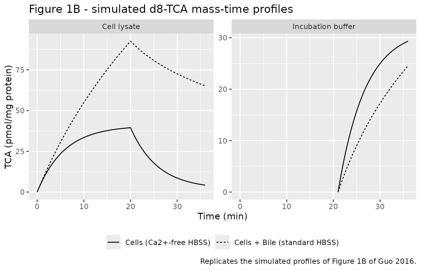
at_time <- function(d, tt) d[which.min(abs(d$time - tt)), ]

cells_20     <- at_time(sim_caf, 20)$cells / PROTEIN_MG_REF
cellsbile_20 <- at_time(sim_std, 20)$xCellsBile / PROTEIN_MG_REF
ctcells_20   <- at_time(sim_caf, 20)$ctCells

# Bounds are wide because the reference values are read off a printed figure,
# not tabulated. Read-offs from Figure 1B at t = 20 min: the simulated Cells
# line sits near 40 pmol/mg protein and the simulated Cells + Bile line near
# 84 pmol/mg protein (its observed mean is higher, near 105 -- the published
# line under-predicts the 20-minute Cells + Bile point, which is visible in the
# paper's own figure). All three checks are deterministic: the model carries no
# random effects, so no cohort is drawn.
stopifnot(
  cells_20     > 30 && cells_20     < 50,
  cellsbile_20 > 70 && cellsbile_20 < 115,
  # Results: "After 20-minute uptake, TCA Ct,Cells was 5.6 uM." That is the
  # observed value; the simulated line runs slightly below it.
  abs(ctcells_20 - 5.6) / 5.6 < 0.10
)

tibble::tibble(
  Quantity = c("Cells at 20 min (pmol/mg protein)",
               "Cells + Bile at 20 min (pmol/mg protein)",
               "Ct,Cells at 20 min (umol/L)"),
  Simulated = round(c(cells_20, cellsbile_20, ctcells_20), 2),
  Published = c("~40 (Fig. 1B line)", "~84 (Fig. 1B line)", "5.6 (Results text)")
) |>
knitr::kable(caption = "Figure 1B read-offs versus the packaged model.")| Quantity | Simulated | Published |
|---|---|---|
| Cells at 20 min (pmol/mg protein) | 39.50 | ~40 (Fig. 1B line) |
| Cells + Bile at 20 min (pmol/mg protein) | 92.58 | ~84 (Fig. 1B line) |
| Ct,Cells at 20 min (umol/L) | 5.34 | 5.6 (Results text) |
Structural checks
Two properties follow from the equations rather than from any fitted value, so they are exact and catch a sign error, a dropped term or a mis-typed clearance immediately.
# 1. Mass balance. With no wash, the well is closed: buffer + cells + bile must
#    equal the administered 300 pmol at every time point.
closed <- solve_schh(schh_well(seq(0, 600, by = 5), ca_free = 0))
total  <- closed$buffer + closed$cells + closed$bile
stopifnot(max(abs(total - DOSE_PMOL)) < 1e-6)

# 2. Steady-state flux identity. Setting eq. 3 to zero gives
#    Ct,Cells / Ct,Buffer = CLUptake / (CLBL + CLBile), independent of every
#    volume and of the protein content.
eq       <- closed[nrow(closed), ]
ratio    <- eq$ctCells / eq$ctBuffer
expected <- 0.63 / (0.034 + 0.074)
stopifnot(abs(ratio - expected) / expected < 1e-4)

tibble::tibble(
  Check = c("Mass balance (max absolute drift, pmol)",
            "Ct,Cells / Ct,Buffer at equilibrium",
            "CLUptake / (CLBL + CLBile) from Table 2"),
  Value = c(signif(max(abs(total - DOSE_PMOL)), 3), round(ratio, 5), round(expected, 5))
) |>
knitr::kable(caption = "Structural checks on the packaged ODE system.")| Check | Value |
|---|---|
| Mass balance (max absolute drift, pmol) | 0.00000 |
| Ct,Cells / Ct,Buffer at equilibrium | 5.83333 |
| CLUptake / (CLBL + CLBile) from Table 2 | 5.83333 |
Figure 2: which model output is sensitive to inhibition?
Figure 2 sweeps the fraction of inhibition of CLUptake and of CLEfflux (= CLBL + CLBile) from 0 to 0.99 and asks which readout of the SCHH assay moves. The paper’s answer is the cellular total concentration Ct,Cells, and it quotes two corner values: Ct,Cells falls to 0.01-fold of baseline when uptake is 99 % inhibited and rises to approximately 15-fold when efflux is 99 % inhibited.
A competitive term CL / (1 + ratio), where
ratio is [I] / IC50, reduces a clearance by
the fraction ratio / (1 + ratio). Setting every IC50 to 1
makes the two inhibitor-concentration covariates act as
ratio directly, which is how the fraction-of-inhibition
sweep is expressed with the packaged model. The IC50s are
fixed() ini() entries, so they are overridden
through params.
frac_to_ratio <- function(f) f / (1 - f)
unit_ic50 <- c(ic50NtcpTel = 1, ic50Oatp1b1Tel = 1, ic50BsepTel = 1, ic50Mrp3Tel = 1)

fractions <- seq(0, 0.99, length.out = 12)
design <- tidyr::expand_grid(f_uptake = fractions, f_efflux = fractions) |>
  dplyr::mutate(id = dplyr::row_number())

ev_fig2 <- dplyr::bind_rows(lapply(seq_len(nrow(design)), function(i) {
  schh_well(c(0, 120), id = design$id[i], ca_free = 0, telmisartan = 1,
            conc_med  = frac_to_ratio(design$f_uptake[i]),
            conc_cell = frac_to_ratio(design$f_efflux[i]))
}))
stopifnot(!anyDuplicated(unique(ev_fig2[, c("id", "time", "evid")])))

sim_fig2 <- solve_schh(ev_fig2, params = unit_ic50)
#> Warning: multi-subject simulation without without 'omega'
ss <- sim_fig2 |>
  dplyr::filter(time == 120) |>
  dplyr::select(id, ctCells) |>
  dplyr::mutate(id = as.integer(as.character(id)))

baseline <- ss$ctCells[ss$id == design$id[design$f_uptake == 0 & design$f_efflux == 0]]
fig2 <- design |>
  dplyr::left_join(ss, by = "id") |>
  dplyr::mutate(fold = ctCells / baseline)

ggplot(fig2, aes(f_uptake, f_efflux, fill = log10(fold))) +
  geom_raster(interpolate = TRUE) +
  scale_fill_viridis_c(option = "C") +
  labs(x = "Fraction of CLUptake inhibited", y = "Fraction of CLEfflux inhibited",
       fill = "log10(fold\nchange)",
       title = "Figure 2A - fold change in TCA Ct,Cells at steady state (120 min)",
       caption = "Replicates panel A of Figure 2 of Guo 2016.")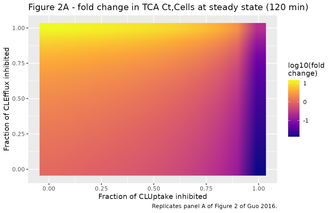
corner <- function(fu, fe) {
  i <- which(abs(fig2$f_uptake - fu) < 1e-9 & abs(fig2$f_efflux - fe) < 1e-9)
  stopifnot(length(i) == 1L)   # a lookup that matches nothing must fail loudly
  fig2$fold[i]
}
fold_uptake_only <- corner(0.99, 0)
fold_efflux_only <- corner(0, 0.99)

# Deterministic quantities -- no random effects anywhere in this model -- so the
# bounds are set from the published claims, not from a tolerance around one run.
stopifnot(
  fold_uptake_only < 0.02,                       # paper: "decreased to 0.01-fold"
  abs(fold_efflux_only - 15) / 15 < 0.15         # paper: "approximately 15-fold"
)

tibble::tibble(
  Scenario  = c("CLUptake 99% inhibited, CLEfflux not inhibited",
                "CLEfflux 99% inhibited, CLUptake not inhibited"),
  Simulated = signif(c(fold_uptake_only, fold_efflux_only), 3),
  Published = c("0.01-fold", "approximately 15-fold")
) |>
knitr::kable(caption = "Figure 2 corner claims versus the packaged model.")| Scenario | Simulated | Published |
|---|---|---|
| CLUptake 99% inhibited, CLEfflux not inhibited | 0.0138 | 0.01-fold |
| CLEfflux 99% inhibited, CLUptake not inhibited | 14.7000 | approximately 15-fold |
Recovering the unreported protein content
The two Figure 2 corners are the only quantities in the paper that
depend appreciably on the per-well protein content, because they are the
only ones driven by how far the medium is depleted over a long
incubation. Sweeping PROTEIN_MG shows that the published
pair is reproduced around 0.2-0.4 mg/well and not at 1-2 mg/well; 0.4
mg/well is also what the reported seeding density of 0.4e6 cells/well
implies at the conventional ~1 mg protein per 10^6 hepatocytes.
protein_corner <- function(p) {
  ev <- dplyr::bind_rows(
    schh_well(c(0, 120), id = 1L, protein_mg = p, telmisartan = 1),
    schh_well(c(0, 120), id = 2L, protein_mg = p, telmisartan = 1,
              conc_med = frac_to_ratio(0.99)),
    schh_well(c(0, 120), id = 3L, protein_mg = p, telmisartan = 1,
              conc_cell = frac_to_ratio(0.99))
  )
  s <- solve_schh(ev, params = unit_ic50) |>
    dplyr::filter(time == 120) |>
    dplyr::mutate(id = as.integer(as.character(id))) |>
    dplyr::arrange(id)
  c(uptake = s$ctCells[2] / s$ctCells[1], efflux = s$ctCells[3] / s$ctCells[1])
}

sweep <- vapply(c(0.1, 0.2, 0.4, 0.67, 1, 1.5, 2), protein_corner, numeric(2))
#> Warning: multi-subject simulation without without 'omega'
#> Warning: multi-subject simulation without without 'omega'
#> Warning: multi-subject simulation without without 'omega'
#> Warning: multi-subject simulation without without 'omega'
#> Warning: multi-subject simulation without without 'omega'
#> Warning: multi-subject simulation without without 'omega'
#> Warning: multi-subject simulation without without 'omega'
tibble::tibble(
  `PROTEIN_MG (mg/well)`             = c(0.1, 0.2, 0.4, 0.67, 1, 1.5, 2),
  `Uptake 99% inhibited (fold)`      = signif(sweep["uptake", ], 3),
  `Efflux 99% inhibited (fold)`      = signif(sweep["efflux", ], 3)
) |>
knitr::kable(caption = "Sensitivity of the Figure 2 corners to the unreported per-well protein content. Published values: 0.01-fold and approximately 15-fold.")| PROTEIN_MG (mg/well) | Uptake 99% inhibited (fold) | Efflux 99% inhibited (fold) |
|---|---|---|
| 0.10 | 0.0109 | 16.80 |
| 0.20 | 0.0118 | 16.10 |
| 0.40 | 0.0138 | 14.70 |
| 0.67 | 0.0164 | 13.30 |
| 1.00 | 0.0198 | 12.00 |
| 1.50 | 0.0249 | 10.60 |
| 2.00 | 0.0299 | 9.77 |
Table 4: predicted versus observed inhibitor effects
The paper pre-incubated SCHH with telmisartan (1 or 10 umol/L) or bosentan (0.8 or 8 umol/L), then co-incubated with 1 umol/L d8-TCA for 10 minutes, and compared the resulting fold change in Ct,Cells against a Monte Carlo prediction: 40 individuals, repeated 10 times, drawing each clearance from a normal distribution with the Table 2 mean and SD.
# Table 3 measured concentrations, and the four candidate intracellular
# quantities the paper substitutes into the same [I]cell slot.
scenarios <- tibble::tribble(
  ~inhibitor,    ~level,  ~conc_med, ~t_cell, ~u_cell, ~t_cyt, ~u_cyt, ~observed,
  "Telmisartan", "1 uM",     0.012,      16,     2.1,     16,   0.85,      0.91,
  "Telmisartan", "10 uM",    0.20,       40,     3.7,     35,   2.8,       1.1,
  "Bosentan",    "0.8 uM",   0.031,     1.9,    0.79,    1.7,   0.21,      0.88,
  "Bosentan",    "8 uM",     0.45,       17,     3.8,     14,   NA,        0.81
)

published <- tibble::tribble(
  ~inhibitor,    ~level,  ~`[I]t,cell`, ~`[I]u,cell`, ~`[I]t,cyt`, ~`[I]u,cyt`,
  "Telmisartan", "1 uM",         1.3,          1.0,         1.3,        1.0,
  "Telmisartan", "10 uM",        1.4,          1.0,         1.3,        0.96,
  "Bosentan",    "0.8 uM",       1.0,         0.99,         1.0,       0.99,
  "Bosentan",    "8 uM",         1.2,          1.0,         1.1,         NA
)
# Monte Carlo over the Table 2 parameter uncertainty. The draws use R's RNG
# (not rxode2's), so unlike a cohort simulated inside rxSolve this is
# reproducible regardless of how many solver threads are available.
set.seed(20160527)
N_IND <- 40L
N_REP <- 10L

TAB2 <- list(cluptake = c(0.63, 0.12), clbl = c(0.034, 0.011),
             clbile   = c(0.074, 0.030), kflux = c(0.018, 0.0015))

# CL was "assumed to be normally distributed" (Methods). A normal draw can go
# non-positive at CV 32-36%; those draws are resampled, which the paper does not
# describe -- see "Assumptions and deviations".
rnorm_pos <- function(n, mean, sd) {
  x <- rnorm(n, mean, sd)
  while (any(x <= 0)) x[x <= 0] <- rnorm(sum(x <= 0), mean, sd)
  x
}

draws <- lapply(seq_len(N_REP), function(rep) {
  data.frame(
    lcluptake = log(rnorm_pos(N_IND, TAB2$cluptake[1], TAB2$cluptake[2])),
    lclbl     = log(rnorm_pos(N_IND, TAB2$clbl[1],     TAB2$clbl[2])),
    lclbile   = log(rnorm_pos(N_IND, TAB2$clbile[1],   TAB2$clbile[2])),
    lkflux    = log(rnorm_pos(N_IND, TAB2$kflux[1],    TAB2$kflux[2]))
  )
})

# 10-minute uptake in standard HBSS, one well per drawn individual.
ev_mc <- dplyr::bind_rows(lapply(seq_len(N_IND), function(i)
  schh_well(c(0, 10), id = i, ca_free = 0)))

# Solve the whole 40-individual replicate in one call, varying only the
# inhibitor covariates between arms.
arm_ctcells <- function(pars, conc_med, conc_cell, telmisartan, bosentan) {
  ev <- ev_mc |>
    dplyr::mutate(CONC_INHIBITOR_MEDIUM_UNBOUND_UM = conc_med,
                  CONC_INHIBITOR_CELL_UM           = conc_cell,
                  CONMED_TELMISARTAN               = telmisartan,
                  CONMED_BOSENTAN                  = bosentan)
  s <- rxode2::rxSolve(mod, params = pars, events = ev, covsInterpolation = "locf",
                       returnType = "data.frame")
  s <- s[s$time == 10, ]
  s$ctCells[order(as.integer(as.character(s$id)))]
}

itypes <- c("[I]t,cell" = "t_cell", "[I]u,cell" = "u_cell",
            "[I]t,cyt" = "t_cyt",  "[I]u,cyt" = "u_cyt")

results <- dplyr::bind_rows(lapply(seq_len(nrow(scenarios)), function(k) {
  sc  <- scenarios[k, ]
  tel <- as.integer(sc$inhibitor == "Telmisartan")
  bos <- as.integer(sc$inhibitor == "Bosentan")
  dplyr::bind_rows(lapply(names(itypes), function(lab) {
    icell <- sc[[itypes[[lab]]]]
    if (is.na(icell)) return(NULL)
    per_rep <- vapply(draws, function(pars) {
      ctrl <- arm_ctcells(pars, 0, 0, tel, bos)
      inh  <- arm_ctcells(pars, sc$conc_med, icell, tel, bos)
      mean(inh / ctrl)                      # mean over the 40 individuals
    }, numeric(1))
    tibble::tibble(inhibitor = sc$inhibitor, level = sc$level, itype = lab,
                   sim = mean(per_rep),     # mean of the 10 simulations
                   lo = quantile(per_rep, 0.025), hi = quantile(per_rep, 0.975))
  }))
}))
#> Warning: multi-subject simulation without without 'omega'
#> Warning: multi-subject simulation without without 'omega'
#> Warning: multi-subject simulation without without 'omega'
#> Warning: multi-subject simulation without without 'omega'
#> Warning: multi-subject simulation without without 'omega'
#> Warning: multi-subject simulation without without 'omega'
#> Warning: multi-subject simulation without without 'omega'
#> Warning: multi-subject simulation without without 'omega'
#> Warning: multi-subject simulation without without 'omega'
#> Warning: multi-subject simulation without without 'omega'
#> Warning: multi-subject simulation without without 'omega'
#> Warning: multi-subject simulation without without 'omega'
#> Warning: multi-subject simulation without without 'omega'
#> Warning: multi-subject simulation without without 'omega'
#> Warning: multi-subject simulation without without 'omega'
#> Warning: multi-subject simulation without without 'omega'
#> Warning: multi-subject simulation without without 'omega'
#> Warning: multi-subject simulation without without 'omega'
#> Warning: multi-subject simulation without without 'omega'
#> Warning: multi-subject simulation without without 'omega'
#> Warning: multi-subject simulation without without 'omega'
#> Warning: multi-subject simulation without without 'omega'
#> Warning: multi-subject simulation without without 'omega'
#> Warning: multi-subject simulation without without 'omega'
#> Warning: multi-subject simulation without without 'omega'
#> Warning: multi-subject simulation without without 'omega'
#> Warning: multi-subject simulation without without 'omega'
#> Warning: multi-subject simulation without without 'omega'
#> Warning: multi-subject simulation without without 'omega'
#> Warning: multi-subject simulation without without 'omega'
#> Warning: multi-subject simulation without without 'omega'
#> Warning: multi-subject simulation without without 'omega'
#> Warning: multi-subject simulation without without 'omega'
#> Warning: multi-subject simulation without without 'omega'
#> Warning: multi-subject simulation without without 'omega'
#> Warning: multi-subject simulation without without 'omega'
#> Warning: multi-subject simulation without without 'omega'
#> Warning: multi-subject simulation without without 'omega'
#> Warning: multi-subject simulation without without 'omega'
#> Warning: multi-subject simulation without without 'omega'
#> Warning: multi-subject simulation without without 'omega'
#> Warning: multi-subject simulation without without 'omega'
#> Warning: multi-subject simulation without without 'omega'
#> Warning: multi-subject simulation without without 'omega'
#> Warning: multi-subject simulation without without 'omega'
#> Warning: multi-subject simulation without without 'omega'
#> Warning: multi-subject simulation without without 'omega'
#> Warning: multi-subject simulation without without 'omega'
#> Warning: multi-subject simulation without without 'omega'
#> Warning: multi-subject simulation without without 'omega'
#> Warning: multi-subject simulation without without 'omega'
#> Warning: multi-subject simulation without without 'omega'
#> Warning: multi-subject simulation without without 'omega'
#> Warning: multi-subject simulation without without 'omega'
#> Warning: multi-subject simulation without without 'omega'
#> Warning: multi-subject simulation without without 'omega'
#> Warning: multi-subject simulation without without 'omega'
#> Warning: multi-subject simulation without without 'omega'
#> Warning: multi-subject simulation without without 'omega'
#> Warning: multi-subject simulation without without 'omega'
#> Warning: multi-subject simulation without without 'omega'
#> Warning: multi-subject simulation without without 'omega'
#> Warning: multi-subject simulation without without 'omega'
#> Warning: multi-subject simulation without without 'omega'
#> Warning: multi-subject simulation without without 'omega'
#> Warning: multi-subject simulation without without 'omega'
#> Warning: multi-subject simulation without without 'omega'
#> Warning: multi-subject simulation without without 'omega'
#> Warning: multi-subject simulation without without 'omega'
#> Warning: multi-subject simulation without without 'omega'
#> Warning: multi-subject simulation without without 'omega'
#> Warning: multi-subject simulation without without 'omega'
#> Warning: multi-subject simulation without without 'omega'
#> Warning: multi-subject simulation without without 'omega'
#> Warning: multi-subject simulation without without 'omega'
#> Warning: multi-subject simulation without without 'omega'
#> Warning: multi-subject simulation without without 'omega'
#> Warning: multi-subject simulation without without 'omega'
#> Warning: multi-subject simulation without without 'omega'
#> Warning: multi-subject simulation without without 'omega'
#> Warning: multi-subject simulation without without 'omega'
#> Warning: multi-subject simulation without without 'omega'
#> Warning: multi-subject simulation without without 'omega'
#> Warning: multi-subject simulation without without 'omega'
#> Warning: multi-subject simulation without without 'omega'
#> Warning: multi-subject simulation without without 'omega'
#> Warning: multi-subject simulation without without 'omega'
#> Warning: multi-subject simulation without without 'omega'
#> Warning: multi-subject simulation without without 'omega'
#> Warning: multi-subject simulation without without 'omega'
#> Warning: multi-subject simulation without without 'omega'
#> Warning: multi-subject simulation without without 'omega'
#> Warning: multi-subject simulation without without 'omega'
#> Warning: multi-subject simulation without without 'omega'
#> Warning: multi-subject simulation without without 'omega'
#> Warning: multi-subject simulation without without 'omega'
#> Warning: multi-subject simulation without without 'omega'
#> Warning: multi-subject simulation without without 'omega'
#> Warning: multi-subject simulation without without 'omega'
#> Warning: multi-subject simulation without without 'omega'
#> Warning: multi-subject simulation without without 'omega'
#> Warning: multi-subject simulation without without 'omega'
#> Warning: multi-subject simulation without without 'omega'
#> Warning: multi-subject simulation without without 'omega'
#> Warning: multi-subject simulation without without 'omega'
#> Warning: multi-subject simulation without without 'omega'
#> Warning: multi-subject simulation without without 'omega'
#> Warning: multi-subject simulation without without 'omega'
#> Warning: multi-subject simulation without without 'omega'
#> Warning: multi-subject simulation without without 'omega'
#> Warning: multi-subject simulation without without 'omega'
#> Warning: multi-subject simulation without without 'omega'
#> Warning: multi-subject simulation without without 'omega'
#> Warning: multi-subject simulation without without 'omega'
#> Warning: multi-subject simulation without without 'omega'
#> Warning: multi-subject simulation without without 'omega'
#> Warning: multi-subject simulation without without 'omega'
#> Warning: multi-subject simulation without without 'omega'
#> Warning: multi-subject simulation without without 'omega'
#> Warning: multi-subject simulation without without 'omega'
#> Warning: multi-subject simulation without without 'omega'
#> Warning: multi-subject simulation without without 'omega'
#> Warning: multi-subject simulation without without 'omega'
#> Warning: multi-subject simulation without without 'omega'
#> Warning: multi-subject simulation without without 'omega'
#> Warning: multi-subject simulation without without 'omega'
#> Warning: multi-subject simulation without without 'omega'
#> Warning: multi-subject simulation without without 'omega'
#> Warning: multi-subject simulation without without 'omega'
#> Warning: multi-subject simulation without without 'omega'
#> Warning: multi-subject simulation without without 'omega'
#> Warning: multi-subject simulation without without 'omega'
#> Warning: multi-subject simulation without without 'omega'
#> Warning: multi-subject simulation without without 'omega'
#> Warning: multi-subject simulation without without 'omega'
#> Warning: multi-subject simulation without without 'omega'
#> Warning: multi-subject simulation without without 'omega'
#> Warning: multi-subject simulation without without 'omega'
#> Warning: multi-subject simulation without without 'omega'
#> Warning: multi-subject simulation without without 'omega'
#> Warning: multi-subject simulation without without 'omega'
#> Warning: multi-subject simulation without without 'omega'
#> Warning: multi-subject simulation without without 'omega'
#> Warning: multi-subject simulation without without 'omega'
#> Warning: multi-subject simulation without without 'omega'
#> Warning: multi-subject simulation without without 'omega'
#> Warning: multi-subject simulation without without 'omega'
#> Warning: multi-subject simulation without without 'omega'
#> Warning: multi-subject simulation without without 'omega'
#> Warning: multi-subject simulation without without 'omega'
#> Warning: multi-subject simulation without without 'omega'
#> Warning: multi-subject simulation without without 'omega'
#> Warning: multi-subject simulation without without 'omega'
#> Warning: multi-subject simulation without without 'omega'
#> Warning: multi-subject simulation without without 'omega'
#> Warning: multi-subject simulation without without 'omega'
#> Warning: multi-subject simulation without without 'omega'
#> Warning: multi-subject simulation without without 'omega'
#> Warning: multi-subject simulation without without 'omega'
#> Warning: multi-subject simulation without without 'omega'
#> Warning: multi-subject simulation without without 'omega'
#> Warning: multi-subject simulation without without 'omega'
#> Warning: multi-subject simulation without without 'omega'
#> Warning: multi-subject simulation without without 'omega'
#> Warning: multi-subject simulation without without 'omega'
#> Warning: multi-subject simulation without without 'omega'
#> Warning: multi-subject simulation without without 'omega'
#> Warning: multi-subject simulation without without 'omega'
#> Warning: multi-subject simulation without without 'omega'
#> Warning: multi-subject simulation without without 'omega'
#> Warning: multi-subject simulation without without 'omega'
#> Warning: multi-subject simulation without without 'omega'
#> Warning: multi-subject simulation without without 'omega'
#> Warning: multi-subject simulation without without 'omega'
#> Warning: multi-subject simulation without without 'omega'
#> Warning: multi-subject simulation without without 'omega'
#> Warning: multi-subject simulation without without 'omega'
#> Warning: multi-subject simulation without without 'omega'
#> Warning: multi-subject simulation without without 'omega'
#> Warning: multi-subject simulation without without 'omega'
#> Warning: multi-subject simulation without without 'omega'
#> Warning: multi-subject simulation without without 'omega'
#> Warning: multi-subject simulation without without 'omega'
#> Warning: multi-subject simulation without without 'omega'
#> Warning: multi-subject simulation without without 'omega'
#> Warning: multi-subject simulation without without 'omega'
#> Warning: multi-subject simulation without without 'omega'
#> Warning: multi-subject simulation without without 'omega'
#> Warning: multi-subject simulation without without 'omega'
#> Warning: multi-subject simulation without without 'omega'
#> Warning: multi-subject simulation without without 'omega'
#> Warning: multi-subject simulation without without 'omega'
#> Warning: multi-subject simulation without without 'omega'
#> Warning: multi-subject simulation without without 'omega'
#> Warning: multi-subject simulation without without 'omega'
#> Warning: multi-subject simulation without without 'omega'
#> Warning: multi-subject simulation without without 'omega'
#> Warning: multi-subject simulation without without 'omega'
#> Warning: multi-subject simulation without without 'omega'
#> Warning: multi-subject simulation without without 'omega'
#> Warning: multi-subject simulation without without 'omega'
#> Warning: multi-subject simulation without without 'omega'
#> Warning: multi-subject simulation without without 'omega'
#> Warning: multi-subject simulation without without 'omega'
#> Warning: multi-subject simulation without without 'omega'
#> Warning: multi-subject simulation without without 'omega'
#> Warning: multi-subject simulation without without 'omega'
#> Warning: multi-subject simulation without without 'omega'
#> Warning: multi-subject simulation without without 'omega'
#> Warning: multi-subject simulation without without 'omega'
#> Warning: multi-subject simulation without without 'omega'
#> Warning: multi-subject simulation without without 'omega'
#> Warning: multi-subject simulation without without 'omega'
#> Warning: multi-subject simulation without without 'omega'
#> Warning: multi-subject simulation without without 'omega'
#> Warning: multi-subject simulation without without 'omega'
#> Warning: multi-subject simulation without without 'omega'
#> Warning: multi-subject simulation without without 'omega'
#> Warning: multi-subject simulation without without 'omega'
#> Warning: multi-subject simulation without without 'omega'
#> Warning: multi-subject simulation without without 'omega'
#> Warning: multi-subject simulation without without 'omega'
#> Warning: multi-subject simulation without without 'omega'
#> Warning: multi-subject simulation without without 'omega'
#> Warning: multi-subject simulation without without 'omega'
#> Warning: multi-subject simulation without without 'omega'
#> Warning: multi-subject simulation without without 'omega'
#> Warning: multi-subject simulation without without 'omega'
#> Warning: multi-subject simulation without without 'omega'
#> Warning: multi-subject simulation without without 'omega'
#> Warning: multi-subject simulation without without 'omega'
#> Warning: multi-subject simulation without without 'omega'
#> Warning: multi-subject simulation without without 'omega'
#> Warning: multi-subject simulation without without 'omega'
#> Warning: multi-subject simulation without without 'omega'
#> Warning: multi-subject simulation without without 'omega'
#> Warning: multi-subject simulation without without 'omega'
#> Warning: multi-subject simulation without without 'omega'
#> Warning: multi-subject simulation without without 'omega'
#> Warning: multi-subject simulation without without 'omega'
#> Warning: multi-subject simulation without without 'omega'
#> Warning: multi-subject simulation without without 'omega'
#> Warning: multi-subject simulation without without 'omega'
#> Warning: multi-subject simulation without without 'omega'
#> Warning: multi-subject simulation without without 'omega'
#> Warning: multi-subject simulation without without 'omega'
#> Warning: multi-subject simulation without without 'omega'
#> Warning: multi-subject simulation without without 'omega'
#> Warning: multi-subject simulation without without 'omega'
#> Warning: multi-subject simulation without without 'omega'
#> Warning: multi-subject simulation without without 'omega'
#> Warning: multi-subject simulation without without 'omega'
#> Warning: multi-subject simulation without without 'omega'
#> Warning: multi-subject simulation without without 'omega'
#> Warning: multi-subject simulation without without 'omega'
#> Warning: multi-subject simulation without without 'omega'
#> Warning: multi-subject simulation without without 'omega'
#> Warning: multi-subject simulation without without 'omega'
#> Warning: multi-subject simulation without without 'omega'
#> Warning: multi-subject simulation without without 'omega'
#> Warning: multi-subject simulation without without 'omega'
#> Warning: multi-subject simulation without without 'omega'
#> Warning: multi-subject simulation without without 'omega'
#> Warning: multi-subject simulation without without 'omega'
#> Warning: multi-subject simulation without without 'omega'
#> Warning: multi-subject simulation without without 'omega'
#> Warning: multi-subject simulation without without 'omega'
#> Warning: multi-subject simulation without without 'omega'
#> Warning: multi-subject simulation without without 'omega'
#> Warning: multi-subject simulation without without 'omega'
#> Warning: multi-subject simulation without without 'omega'
#> Warning: multi-subject simulation without without 'omega'
#> Warning: multi-subject simulation without without 'omega'
#> Warning: multi-subject simulation without without 'omega'
#> Warning: multi-subject simulation without without 'omega'
#> Warning: multi-subject simulation without without 'omega'
#> Warning: multi-subject simulation without without 'omega'
#> Warning: multi-subject simulation without without 'omega'
#> Warning: multi-subject simulation without without 'omega'
#> Warning: multi-subject simulation without without 'omega'
#> Warning: multi-subject simulation without without 'omega'
#> Warning: multi-subject simulation without without 'omega'
#> Warning: multi-subject simulation without without 'omega'
#> Warning: multi-subject simulation without without 'omega'
#> Warning: multi-subject simulation without without 'omega'
#> Warning: multi-subject simulation without without 'omega'
#> Warning: multi-subject simulation without without 'omega'
#> Warning: multi-subject simulation without without 'omega'
#> Warning: multi-subject simulation without without 'omega'
#> Warning: multi-subject simulation without without 'omega'
#> Warning: multi-subject simulation without without 'omega'
#> Warning: multi-subject simulation without without 'omega'
#> Warning: multi-subject simulation without without 'omega'
#> Warning: multi-subject simulation without without 'omega'
#> Warning: multi-subject simulation without without 'omega'
#> Warning: multi-subject simulation without without 'omega'
#> Warning: multi-subject simulation without without 'omega'
#> Warning: multi-subject simulation without without 'omega'
#> Warning: multi-subject simulation without without 'omega'
#> Warning: multi-subject simulation without without 'omega'
tab4 <- results |>
  dplyr::left_join(
    published |> tidyr::pivot_longer(-c(inhibitor, level),
                                     names_to = "itype", values_to = "pub"),
    by = c("inhibitor", "level", "itype")
  ) |>
  dplyr::left_join(scenarios |> dplyr::select(inhibitor, level, observed),
                   by = c("inhibitor", "level")) |>
  dplyr::mutate(
    Simulated = sprintf("%.2f (%.2f-%.2f)", sim, lo, hi),
    Published = sprintf("%.2f", pub),
    Delta     = round(sim - pub, 3)
  )

stopifnot(nrow(tab4) == 15L, !anyNA(tab4$pub))     # all 15 published cells present
# Deterministic given set.seed() above; the residual spread is Monte Carlo
# sampling noise on 400 draws against values the paper prints to two
# significant figures.
stopifnot(max(abs(tab4$Delta)) < 0.12)

tab4 |>
  dplyr::select(inhibitor, level, observed, itype, Simulated, Published, Delta) |>
  dplyr::rename("Inhibitor" = inhibitor, "Dosing concentration" = level,
                "Observed" = observed, "Inhibitor concentration used" = itype) |>
  knitr::kable(
    caption = "Table 4 - fold change in TCA Ct,Cells after a 10-minute uptake. Simulated values are the mean of 10 Monte Carlo simulations of 40 individuals (2.5th-97.5th percentile across the 10 simulations); Published is the corresponding cell of Table 4 of Guo 2016.",
    align = c("l", "l", "r", "l", "r", "r", "r")
)| Inhibitor | Dosing concentration | Observed | Inhibitor concentration used | Simulated | Published | Delta |
|---|---|---|---|---|---|---|
| Telmisartan | 1 uM | 0.91 | [I]t,cell | 1.29 (1.27-1.31) | 1.30 | -0.010 |
| Telmisartan | 1 uM | 0.91 | [I]u,cell | 1.05 (1.04-1.05) | 1.00 | 0.048 |
| Telmisartan | 1 uM | 0.91 | [I]t,cyt | 1.29 (1.27-1.31) | 1.30 | -0.010 |
| Telmisartan | 1 uM | 0.91 | [I]u,cyt | 1.02 (1.01-1.02) | 1.00 | 0.016 |
| Telmisartan | 10 uM | 1.10 | [I]t,cell | 1.37 (1.33-1.40) | 1.40 | -0.030 |
| Telmisartan | 10 uM | 1.10 | [I]u,cell | 0.99 (0.99-1.00) | 1.00 | -0.007 |
| Telmisartan | 10 uM | 1.10 | [I]t,cyt | 1.34 (1.31-1.37) | 1.30 | 0.041 |
| Telmisartan | 10 uM | 1.10 | [I]u,cyt | 0.97 (0.97-0.98) | 0.96 | 0.014 |
| Bosentan | 0.8 uM | 0.88 | [I]t,cell | 1.03 (1.03-1.03) | 1.00 | 0.030 |
| Bosentan | 0.8 uM | 0.88 | [I]u,cell | 1.01 (1.01-1.01) | 0.99 | 0.022 |
| Bosentan | 0.8 uM | 0.88 | [I]t,cyt | 1.03 (1.03-1.03) | 1.00 | 0.027 |
| Bosentan | 0.8 uM | 0.88 | [I]u,cyt | 1.00 (1.00-1.00) | 0.99 | 0.012 |
| Bosentan | 8 uM | 0.81 | [I]t,cell | 1.21 (1.19-1.22) | 1.20 | 0.006 |
| Bosentan | 8 uM | 0.81 | [I]u,cell | 1.04 (1.04-1.04) | 1.00 | 0.042 |
| Bosentan | 8 uM | 0.81 | [I]t,cyt | 1.17 (1.16-1.18) | 1.10 | 0.074 |
Every one of the fifteen reproducible cells of Table 4 is recovered
to the two significant figures the paper prints. The pattern the paper
draws out survives: for telmisartan the unbound concentrations give an
average fold error of ~1.0 whereas the total concentrations
over-predict, while for bosentan the choice barely matters. That
difference tracks the intracellular unbound fraction – 0.09-0.13 for
telmisartan against 0.22-0.41 for bosentan – and the paper’s
[I]t,cell / IC50 yardstick, 3.6 for telmisartan at 10
umol/L against 0.8 for bosentan at 8 umol/L.
afe <- tab4 |>
  dplyr::group_by(Inhibitor = inhibitor, `Inhibitor concentration used` = itype) |>
  dplyr::summarise(AFE = 10^mean(log10(sim / observed)), .groups = "drop") |>
  dplyr::mutate(AFE = round(AFE, 2))

published_afe <- tibble::tribble(
  ~Inhibitor,    ~`Inhibitor concentration used`, ~`Published AFE`,
  "Telmisartan", "[I]t,cell", 1.4,
  "Telmisartan", "[I]u,cell", 1.0,
  "Telmisartan", "[I]t,cyt",  1.3,
  "Telmisartan", "[I]u,cyt",  0.99,
  "Bosentan",    "[I]t,cell", 1.3,
  "Bosentan",    "[I]u,cell", 1.2,
  "Bosentan",    "[I]t,cyt",  1.3
)

afe_cmp <- dplyr::inner_join(afe, published_afe,
                             by = c("Inhibitor", "Inhibitor concentration used"))
stopifnot(nrow(afe_cmp) == 7L)                 # guard the join
stopifnot(max(abs(afe_cmp$AFE - afe_cmp$`Published AFE`)) < 0.15)

knitr::kable(afe_cmp, caption = "Average fold error (eq. 11) versus Table 4 of Guo 2016. The bosentan [I]u,cyt cell is not available in the source.")| Inhibitor | Inhibitor concentration used | AFE | Published AFE |
|---|---|---|---|
| Bosentan | [I]t,cell | 1.32 | 1.30 |
| Bosentan | [I]t,cyt | 1.30 | 1.30 |
| Bosentan | [I]u,cell | 1.22 | 1.20 |
| Telmisartan | [I]t,cell | 1.33 | 1.40 |
| Telmisartan | [I]t,cyt | 1.31 | 1.30 |
| Telmisartan | [I]u,cell | 1.02 | 1.00 |
| Telmisartan | [I]u,cyt | 0.99 | 0.99 |
Assumptions and deviations
-
Per-well cellular protein content (
PROTEIN_MG) is not reported. The Methods state that VCells was computed from “the protein content of each preparation”, but no value is tabulated, and it is needed to reconcile the absolute per-well buffer volume (0.3 mL) with the per-mg-protein cellular volume and clearances. This vignette uses 0.4 mg/well, recovered by inverting the paper’s own two Figure 2 fold-change claims (reproduced only around 0.2-0.4 mg/well; see the sweep above) and independently consistent with the reported seeding density of 0.4e6 cells/well. This is non-paper-derived provenance: no model parameter was adjusted, but the value is inferred from published simulation outputs rather than printed. The Table 4 fold changes – the paper’s primary quantitative result – are insensitive to it across at least 0.1-2 mg/well. -
The residual-error model is not reproducible.
Fitting used “a power model to account for residual error” in Phoenix
WinNonlin, but neither the coefficient nor the exponent is reported.
propSdis thereforefixed(0); the packaged model predicts without residual error. -
No between-donor random effects. The three SCHH
preparations were fitted separately and Table 2 reports the mean and SD
across the three fits, not a hierarchical variance. The model carries no
etaterms; the Table 4 section propagates the Table 2 SDs by Monte Carlo, as the paper does. - Non-positive normal draws are resampled. The paper assumed the clearances are normally distributed but does not say how it handled the negative draws that a CV of 32-36 % produces. Resampling is used here; roughly one draw in 400 is affected, which is well below the two significant figures Table 4 reports.
-
Equation 9 (MRP4) is not encoded. The paper
simulated two extremes for the basolateral efflux transporter, 100 %
MRP3 (eq. 8) or 100 % MRP4 (eq. 9), found “the simulation results were
similar”, and selected MRP3 for every reported simulation. Eq. 9 is
therefore a robustness check rather than a reported final model, and is
excluded. The Table 1 MRP4 potencies (telmisartan 11-36 umol/L, bosentan
22 umol/L) are consequently not carried in
ini(). - Ranges in Table 1 are entered as the mean of their endpoints, following the Methods statement that “the mean IC50 values for each transporter in Table 1 were used”. This affects telmisartan BSEP (16-16.2 -> 16.1), bosentan BSEP (23-42 -> 32.5) and bosentan NTCP (18 and 36 -> 27). Bosentan OATP1B1 is taken as the printed 18 umol/L, per Table 1’s footnote a (“Not available and therefore assumed to be the same as NTCP”).
- Supplemental Figure 1 was not obtainable. The article is not open access, and the supplement was not available when this model was built. The figure shows a simulation of how telmisartan’s effect grows as the uptake phase is extended, generated from equations and parameter values that are all in the main text, so no parameter is missing. The one claim that depends on it – “After a 30-minute uptake phase, the simulated TCA Ct,Cells for telmisartan based on [I]t,cell was threefold of the simulation based on [I]u,cyt” – is not asserted here; the packaged model gives about twofold at 30 minutes for the 10 umol/L level.
- The observed Cells + Bile point at 20 minutes is under-predicted, by the packaged model and by the paper’s own Figure 1B line alike (line ~84 against an observed mean ~105 pmol/mg protein). The paper attributes the Figure 1B lines to “the mean of best-fit parameter estimates from three SCHH datasets”, and a mean-of-parameters simulation is not the mean of three simulations, so the two need not agree.