mRNA-encoded BiTE multiscale PBPK (Fiandaca 2025)
Source:vignettes/articles/Fiandaca_2025_mRNABiTE.Rmd
Fiandaca_2025_mRNABiTE.RmdModel and source
- Citation: Fiandaca G, Campanile E, Leonardelli L, Pettina E, Giampiccolo S, Carstens EJ, Dasti L, Zangani N, Marchetti L. A multiscale physiologically based pharmacokinetic model to support mRNA-encoded BiTE therapy in cancer treatment. Mol Ther Nucleic Acids. 2025;36(3):102606. doi:10.1016/j.omtn.2025.102606. MATLAB source deposited by the authors at https://github.com/cosbi-research/PBPKmRNABiTE (Data and code availability); every physiological constant and fitted estimate in this file is traced to that deposit and/or paper Table 1.
- Article: https://doi.org/10.1016/j.omtn.2025.102606
- Author source code (Data and code availability): https://github.com/cosbi-research/PBPKmRNABiTE
Fiandaca et al. couple two modules. The protein-transport module (PTM) is the Li and Shah (2019) two-pore whole-body PBPK platform: 15 tissues plus a tumour, each split into vascular, endosomal and interstitial sub-compartments, linked by plasma flow and a lymphatic return. Because a BiTE carries no Fc sequence, the authors deliberately drop FcRn recycling, so each tissue endosome is a pure degradation sink. The mRNA-transport module (MTM) sits on top: mRNA dosed intravenously in a liver-tropic ionizable lipid nanoparticle migrates to the liver and passes through a short chain of intracellular states, each translating BiTE directly into the hepatic interstitium.
The paper reports two variants of the MTM, and this package ships both:
scm <- readModelDb("Fiandaca_2025_mRNABiTE_scm")()
lcm <- readModelDb("Fiandaca_2025_mRNABiTE_lcm")()
c(SCM_states = length(scm$state), LCM_states = length(lcm$state))
#> SCM_states LCM_states
#> 53 54-
Fiandaca_2025_mRNABiTE_scm– the short-chain model (SCM), two liver mRNA states, 53 ODEs (paper Equations 1-4, Figure 3). -
Fiandaca_2025_mRNABiTE_lcm– the long-chain model (LCM), three liver mRNA states, 54 ODEs (paper Equations 5-9, Figure 6A). The third state was added because the observed serum profile shows two peaks, i.e. three changes of slope.
Both files also serve the recombinant BiTE: dose
plasma instead of mrna_plasma and the mRNA
states stay at zero, which is exactly the authors’ separate
recombinant_model.m.
Units
Doses are in ug and all ODE states are
amounts in ug; sub-compartment volumes are in
L, so every concentration formed in
model() is ug/L, i.e. ng/mL – the units
Huang et al. report serum BiTE in. checkModelConventions()
raises an informational note that the dosing and concentration
magnitudes differ; that is intended and no scaling term is needed.
Writing the mRNA chain in amounts rather than the deposit’s
concentrations makes the V_BL^TOT / V_LV^IS ratio of
Equations 2 and 6 cancel exactly, so no volume term appears in the mRNA
ODEs.
Population
pop <- readModelDb("Fiandaca_2025_mRNABiTE_scm")()$population
str(pop, max.level = 1, give.attr = FALSE)
#> List of 9
#>  $ species      : chr "mouse (8-10 weeks old, immunodeficient, tumour-bearing)"
#>  $ n_subjects   : int NA
#>  $ n_studies    : int 1
#>  $ age_range    : chr "8-10 weeks"
#>  $ weight_range : chr "0.028 kg used for the physiological parameter set (deposit pars.BW); the dose calculation in the deposit simula"| __truncated__
#>  $ disease_state: chr "Subcutaneous tumour-bearing immunodeficient mice; a 0.472 mL tumour is carried as a 16th perfused tissue."
#>  $ dose_range   : chr "Single IV bolus. Recombinant BiTE 6 mg/kg (120 ug). mRNA-BiTE 1.5 mg/kg (30 ug) for training; 0.5, 1, 1.5 and 2"| __truncated__
#>  $ notes        : chr "Training and validation data are the published mouse serum BiTE profiles of Huang et al. 2023 (the B7H3 x CD3 B"| __truncated__
#>  $ scope_note   : chr "Deterministic mechanistic platform: no between-subject random effects and no residual-error magnitude are repor"| __truncated__
The model was calibrated to the mouse experiments of Huang et al. (2023): 8-10 week old immunodeficient, tumour-bearing mice given a single intravenous dose of either 6 mg/kg (120 ug) recombinant B7H3 x CD3 BiTE or 1.5 mg/kg (30 ug) of the LNP-formulated mRNA encoding it. Serum BiTE was measured at 1, 4, 6, 12, 24, 48, 72, 144 and 168 h. A separate dose-escalation experiment gave 0.5, 1, 1.5 and 2 mg/kg mRNA-BiTE with a single 24 h sample per animal; those data are the validation set (paper Figures 5 and 6C).
Serum was treated as equivalent to plasma, which the authors justify on the grounds that BiTEs do not bind clotting factors appreciably (Materials and methods, “Data”).
The physiological parameter set is the 28 g mouse of Li and Shah
(2019) / Shah and Betts (2012). Note that the deposit’s dose arithmetic
uses a 0.02 kg mouse (6 * 0.02 mg), which is what
reproduces the absolute doses Huang et al. report; the two body weights
are used for different purposes and are carried through unchanged.
Source trace
Every ini() entry carries an in-file comment naming its
origin. The authors deposited their complete MATLAB source, so each
value can be traced to both the paper and an executable line.
| Quantity | Value (SCM / LCM) | Source |
|---|---|---|
lkbl2lv mRNA blood-to-liver migration |
6.804e-1 / 1 | Table 1; *_parameters_estimated.mat[2]
|
lks12 first-to-second mRNA state |
4.807e-1 / 1.03e-1 | Table 1; .mat[6] / .mat[7]
|
lks23 second-to-third mRNA state |
– / 2.44e-2 | Table 1; .mat[8]
|
lkrna mRNA clearance |
1.08e-2 / 2.94e-2 | Table 1; .mat[3]
|
lktr_mrna1 translation, state 1 |
9.682e-1 / 6.816e-1 | Table 1; .mat[4]
|
lktr_mrna2 translation, state 2 |
3.182e-1 / 1.01e-2 | Table 1; .mat[5]
|
lktr_mrna3 translation, state 3 |
– / 1.574 | Table 1; .mat[6]
|
lclup pinocytosis rate |
1e-1 / 1e-3 | Table 1; .mat[1]
|
lfrac_mrna_other non-liver mRNA fraction |
0.011 | Results, “Model training and validation”;
pars.ratio_in_other
|
lkdeg endosomal degradation |
32.2 /h |
SCM_simulation.m K_deg, cited to Li and
Shah 2019 |
lclnlf lymph-node flow scaling |
9.1 |
SCM_simulation.m C_LNLF, cited to Shah and
Betts 2012 |
| Organ volumes, plasma flows, tumour fractions | see model()
|
SCM_parameters_collection_mouse.m |
55 kDa two-pore constants (a_e, theta,
Pe_S, Pe_L, alpha_L,
alpha_S, X_J, Xp, pore
areas) |
see model()
|
Parameters_collection_BiTEs_55kDa.m (Li and Shah 2019
Table 4, 55 kDa row) |
| mRNA ODEs | Equations 1-3 (SCM) / 5-8 (LCM) | paper p.4, p.7 |
| Hepatic BiTE production | Equation 4 (SCM) / 9 (LCM) | paper p.4, p.7 |
| Tissue vascular / endosomal / interstitial / plasma / lymph ODEs | Equations 1-5, 7 of Li and Shah 2019 | deposit SCM.m dydt(1:50)
|
Table 1 in the PDF prints the estimates in scientific notation; the
deposited .mat files carry the same values at full
precision and are used here, with the rounded published value recorded
alongside in each comment.
Observed data
The digitised training and validation data are transcribed from the
deposit’s simulation drivers (SCM_simulation.m,
LCM_simulation.m), which is where the authors themselves
store the Huang et al. (2023) means and confidence limits.
t_obs <- c(1, 4, 6, 12, 24, 48, 72, 144, 168)

obs_recombinant <- tibble::tibble(
  time  = t_obs,
  mean  = c(6227.3, 1772.7, 1090.9, 295.5, 204.5, 90.9, 90.9, 45.5, 45.5),
  upper = c(7772.7, 2181.8, 1454.5, 409.1, 318.2, 204.5, 181.8, 136.4, 90.9),
  lower = c(4681.8, 1272.7, 727.3, 159.1, 0, 0, 0, 0, 0)
)

obs_mrna <- tibble::tibble(
  time  = t_obs,
  mean  = c(0, 3221.1, 6463.2, 5284.2, 4547.4, 3957.9, 3136.8, 547.4, 84.2),
  upper = c(378.9, 3894.7, 7557.9, 5957.9, 5157.9, 4421.1, 4168.4, 842.1, 84.2),
  lower = c(0, 2547.4, 5368.4, 4589.5, 3957.9, 3536.8, 2147.4, 231.6, 0)
)
Simulation helpers
Observation rows point at plasma, a declared ODE state;
Cc is returned as an output column automatically.
DOSE_UG <- function(mg_per_kg) mg_per_kg * 0.02 * 1000   # 0.02 kg mouse, mg -> ug

sim_profile <- function(model, cmt, dose_ug, times = seq(0, 168, by = 0.5)) {
  ev <-
    rxode2::et(amt = dose_ug, cmt = cmt, time = 0) |>
    rxode2::et(time = sort(unique(c(0, times, t_obs))), cmt = "plasma")
  rxode2::rxSolve(model, ev, returnType = "data.frame", useLinCmt = FALSE,
                  atol = 1e-12, rtol = 1e-10) |>
    dplyr::filter(!is.na(Cc)) |>
    dplyr::select(time, Cc)
}
Note the et(time = ..., cmt = ...) form. Passing the
observation grid as a data.frame to et()
instead silently yields a different, shorter grid with no error
and no warning, which would quietly break every comparison below.
Replicating Figure 4A – recombinant BiTE training
Dosing plasma reduces either model to the pure
protein-transport module.
rec <- sim_profile(scm, "plasma", DOSE_UG(6))

ggplot(rec, aes(time, Cc)) +
  geom_line(colour = "#001a66", linewidth = 1) +
  geom_pointrange(data = obs_recombinant,
                  aes(time, mean, ymin = lower, ymax = upper),
                  colour = "#80b3e6", inherit.aes = FALSE) +
  coord_cartesian(ylim = c(0, 8000)) +
  labs(x = "time (h)", y = "BiTE concentration (ng/mL)",
       title = "Replicates Figure 4A of Fiandaca 2025",
       subtitle = "Recombinant BiTE, 6 mg/kg IV; points are Huang 2023 mean and range")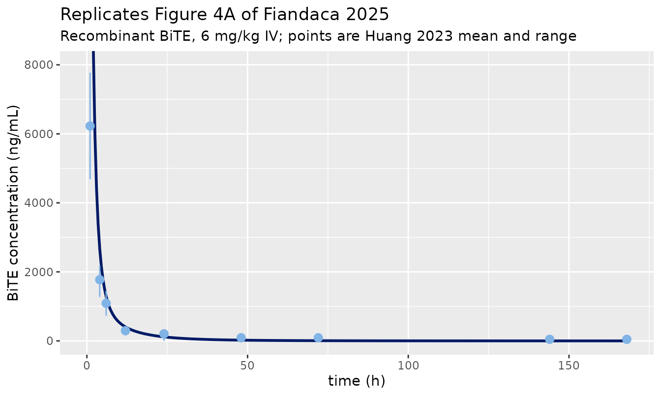
As in the published Figure 4A, the model curve leaves the top of the
axis: the whole 120 ug dose is placed in 0.944 mL of plasma, so
Cc(0) is about 127,072 ng/mL, and the profile falls steeply
through the observed points.
Replicating Figure 4B and 6B – mRNA-encoded BiTE training
mrna_scm <- sim_profile(scm, "mrna_plasma", DOSE_UG(1.5))
mrna_lcm <- sim_profile(lcm, "mrna_plasma", DOSE_UG(1.5))

both <- dplyr::bind_rows(
  dplyr::mutate(mrna_scm, model = "SCM (Figure 4B)"),
  dplyr::mutate(mrna_lcm, model = "LCM (Figure 6B)")
)

ggplot(both, aes(time, Cc, colour = model)) +
  geom_line(linewidth = 1) +
  geom_pointrange(data = obs_mrna, aes(time, mean, ymin = lower, ymax = upper),
                  colour = "grey30", inherit.aes = FALSE) +
  labs(x = "time (h)", y = "BiTE concentration (ng/mL)", colour = NULL,
       title = "Replicates Figures 4B and 6B of Fiandaca 2025",
       subtitle = "mRNA-BiTE 1.5 mg/kg IV; points are Huang 2023 mean and range")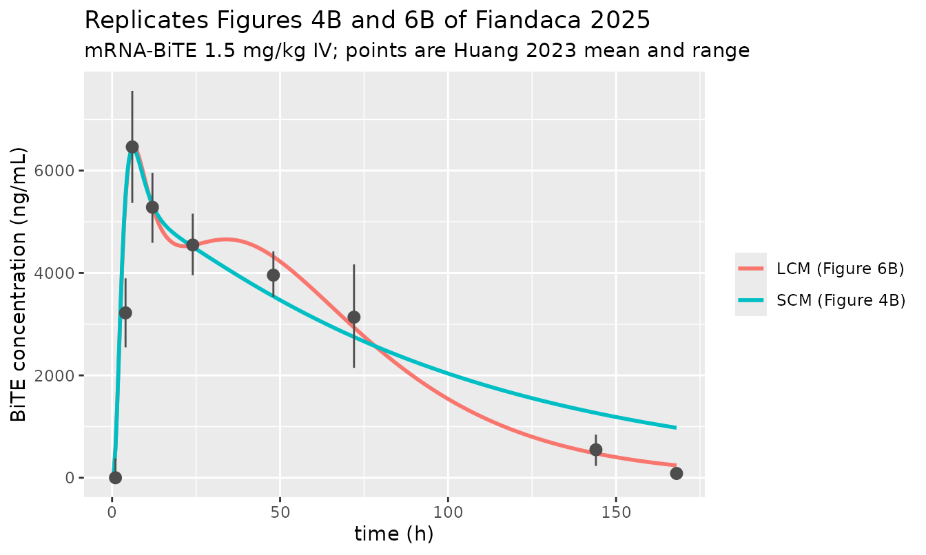
pick <- function(d) d$Cc[match(t_obs, d$time)]
train_tab <- tibble::tibble(
  `Time (h)` = t_obs,
  `Observed (ng/mL)` = obs_mrna$mean,
  `SCM` = round(pick(mrna_scm), 1),
  `LCM` = round(pick(mrna_lcm), 1)
)
knitr::kable(train_tab, caption = "mRNA-BiTE training profile, simulated vs observed")| Time (h) | Observed (ng/mL) | SCM | LCM |
|---|---|---|---|
| 1 | 0.0 | 581.1 | 585.5 |
| 4 | 3221.1 | 5524.6 | 5453.2 |
| 6 | 6463.2 | 6426.8 | 6443.5 |
| 12 | 5284.2 | 5337.4 | 5295.0 |
| 24 | 4547.4 | 4511.6 | 4541.4 |
| 48 | 3957.9 | 3543.8 | 4318.2 |
| 72 | 3136.8 | 2749.8 | 2937.1 |
| 144 | 547.4 | 1265.7 | 474.9 |
| 168 | 84.2 | 976.1 | 241.6 |
Both variants track the observed rise and the 6 h peak closely. The two deficiencies the authors themselves report are reproduced exactly:
- The SCM “slightly overestimates antibody concentrations in the latter part of the observed time frame”, visible here as 976 ng/mL against an observed 84 ng/mL at 168 h.
- The LCM “exhibits improved performance in blood clearance”: at 144 h it gives 475 ng/mL against the SCM’s 1266 ng/mL, with 547 ng/mL observed.
stopifnot(
  # peak within 10% of the observed 6 h maximum, both variants
  abs(max(mrna_scm$Cc) - 6463.2) / 6463.2 < 0.10,
  abs(max(mrna_lcm$Cc) - 6463.2) / 6463.2 < 0.10,
  # the LCM must clear faster than the SCM late, which is why it was built
  pick(mrna_lcm)[8] < pick(mrna_scm)[8],
  pick(mrna_lcm)[9] < pick(mrna_scm)[9]
)
Replicating Figures 5 and 6C – dose-escalation validation
The validation experiment sampled serum BiTE once, at 24 h, after 0.5, 1, 1.5 and 2 mg/kg of mRNA-BiTE.
doses <- c(0.5, 1, 1.5, 2)
esc <- lapply(doses, function(d) {
  tibble::tibble(
    dose_mg_kg = d,
    SCM = sim_profile(scm, "mrna_plasma", DOSE_UG(d), times = c(0, 24)) |>
      dplyr::filter(time == 24) |> dplyr::pull(Cc),
    LCM = sim_profile(lcm, "mrna_plasma", DOSE_UG(d), times = c(0, 24)) |>
      dplyr::filter(time == 24) |> dplyr::pull(Cc)
  )
}) |> dplyr::bind_rows()

knitr::kable(
  esc |> dplyr::mutate(dplyr::across(c(SCM, LCM), ~ round(.x, 1))) |>
    dplyr::rename("mRNA dose (mg/kg)" = dose_mg_kg,
                  "SCM C24 (ng/mL)" = SCM, "LCM C24 (ng/mL)" = LCM),
  caption = "Replicates Figure 5 (SCM) and Figure 6C (LCM): plasma BiTE 24 h after dosing"
)| mRNA dose (mg/kg) | SCM C24 (ng/mL) | LCM C24 (ng/mL) |
|---|---|---|
| 0.5 | 1503.9 | 1513.8 |
| 1.0 | 3007.8 | 3027.6 |
| 1.5 | 4511.6 | 4541.4 |
| 2.0 | 6015.5 | 6055.2 |
The 1.5 mg/kg arm is the training dose, where the observed mean was 4547 ng/mL; the SCM predicts 4512 and the LCM 4541 ng/mL.
Both modules are linear in dose, so the model makes an exact structural prediction: the 24 h concentration must be strictly proportional to the dose. This is a much stronger assertion than “within the experimental variance”, and it is what the paper’s Discussion appeals to when it notes that “protein expression follows a linear dose dependence”.
ratio_scm <- esc$SCM / esc$dose_mg_kg
ratio_lcm <- esc$LCM / esc$dose_mg_kg
stopifnot(
  max(abs(ratio_scm / ratio_scm[1] - 1)) < 1e-6,
  max(abs(ratio_lcm / ratio_lcm[1] - 1)) < 1e-6
)
round(c(SCM_ng_mL_per_mg_kg = ratio_scm[1], LCM_ng_mL_per_mg_kg = ratio_lcm[1]), 1)
#> SCM_ng_mL_per_mg_kg LCM_ng_mL_per_mg_kg
#>              3007.8              3027.6
Structural checks on the mRNA module
Two quantitative claims in the paper can be checked directly against the packaged model rather than against a figure.
Liver targeting. The Results state that the
non-liver fraction was “set to 0.011 based on Huang et al. (2023),
indicating that approximately 99% of administered mRNA accumulates in
the liver after 6 h”. In the model the fraction of the dose that ever
reaches the liver is
kbl2lv / (kbl2lv + krna) * (1 - frac_mrna_other), because
mRNA in blood is lost in parallel to liver uptake and degradation.
p_scm <- scm$theta
frac_to_liver <- function(th) {
  kbl2lv <- exp(th[["lkbl2lv"]]); krna <- exp(th[["lkrna"]])
  kbl2lv / (kbl2lv + krna) * (1 - exp(th[["lfrac_mrna_other"]]))
}
round(c(SCM = frac_to_liver(scm$theta), LCM = frac_to_liver(lcm$theta)), 4)
#>    SCM    LCM
#> 0.9735 0.9608
The SCM delivers 97.4% of the dose to the liver and the LCM 96.1%,
against the paper’s “approximately 99%”. The shortfall is the parallel
blood-side degradation term k_d in Equation 1, which the
0.011 figure from Huang et al. does not account for;
1 - frac_mrna_other alone is 98.9%.
Whole-body mRNA half-life. The paper reports that the fitted degradation rate implies “the corresponding average half-life for the whole-body mRNA concentration resulted in around 45 h”. Total body mRNA is the sum of the plasma and liver states; below is the time at which it has fallen to half the dose.
total_mrna <- function(model, mrna_states, dose_ug = DOSE_UG(1.5)) {
  ev <- rxode2::et(amt = dose_ug, cmt = "mrna_plasma", time = 0) |>
    rxode2::et(time = seq(0, 400, by = 0.25), cmt = "plasma")
  s <- rxode2::rxSolve(model, ev, returnType = "data.frame", useLinCmt = FALSE,
                       atol = 1e-12, rtol = 1e-10)
  tibble::tibble(time = s$time, total = rowSums(s[, mrna_states, drop = FALSE]))
}
half_time <- function(d, dose_ug = DOSE_UG(1.5)) {
  stats::approx(x = d$total, y = d$time, xout = dose_ug / 2)$y
}
tm_scm <- total_mrna(scm, c("mrna_plasma", "mrna_liver1", "mrna_liver2"))
tm_lcm <- total_mrna(lcm, c("mrna_plasma", "mrna_liver1", "mrna_liver2", "mrna_liver3"))
round(c(SCM_t_half_h = half_time(tm_scm), LCM_t_half_h = half_time(tm_lcm),
        SCM_terminal_h = log(2) / exp(scm$theta[["lkrna"]]),
        LCM_terminal_h = log(2) / exp(lcm$theta[["lkrna"]])), 1)
#>   SCM_t_half_h   LCM_t_half_h SCM_terminal_h LCM_terminal_h
#>           62.9           23.2           64.0           23.6
This claim does not reproduce. The packaged SCM
takes about 63 h to clear half the dosed mRNA, essentially its terminal
log(2) / k_d of 64 h – the two agree because almost all the
mRNA sits in the slow second state within a couple of hours. There is no
quantity in the SCM that is close to 45 h.
The likeliest explanation is a factor-of-log(2) slip:
0.5 / k_d is 46 h, which would round to the quoted “around
45 h”, whereas the half-life is log(2) / k_d. Nothing
downstream depends on it – the sentence is a plausibility remark about
the fitted k_d and no parameter is derived from it – but
the figure should not be relied on. It is recorded in the deviations
below.
PKNCA validation
Non-compartmental analysis of the simulated plasma profiles. The
mRNA-BiTE arm is an input-limited profile with a 6 h peak, so
tmax and cmax are the informative checks; the
recombinant arm is a conventional IV bolus.
nca_input <- dplyr::bind_rows(
  dplyr::mutate(sim_profile(scm, "plasma", DOSE_UG(6)),
                id = 1L, treatment = "Recombinant 6 mg/kg (SCM)"),
  dplyr::mutate(mrna_scm, id = 2L, treatment = "mRNA-BiTE 1.5 mg/kg (SCM)"),
  dplyr::mutate(mrna_lcm, id = 3L, treatment = "mRNA-BiTE 1.5 mg/kg (LCM)")
) |>
  dplyr::filter(!is.na(Cc))

dose_input <- tibble::tibble(
  id = 1:3,
  treatment = c("Recombinant 6 mg/kg (SCM)", "mRNA-BiTE 1.5 mg/kg (SCM)",
                "mRNA-BiTE 1.5 mg/kg (LCM)"),
  amt = c(DOSE_UG(6), DOSE_UG(1.5), DOSE_UG(1.5)),
  time = 0
)

conc_obj <- PKNCA::PKNCAconc(nca_input, Cc ~ time | id / treatment)
dose_obj <- PKNCA::PKNCAdose(dose_input, amt ~ time | id)
res <- PKNCA::pk.nca(PKNCA::PKNCAdata(conc_obj, dose_obj))

nca_tab <- as.data.frame(res) |>
  dplyr::filter(PPTESTCD %in% c("cmax", "tmax", "auclast", "half.life")) |>
  dplyr::select(treatment, PPTESTCD, PPORRES) |>
  tidyr::pivot_wider(names_from = PPTESTCD, values_from = PPORRES) |>
  dplyr::mutate(dplyr::across(where(is.numeric), ~ signif(.x, 4)))

knitr::kable(
  nca_tab |> dplyr::rename("Treatment" = treatment, "Cmax (ng/mL)" = cmax,
                           "Tmax (h)" = tmax, "AUClast (ng*h/mL)" = auclast,
                           "t1/2 (h)" = half.life),
  caption = "PKNCA summary of the simulated plasma profiles"
)| Treatment | AUClast (ng*h/mL) | Cmax (ng/mL) | Tmax (h) | t1/2 (h) |
|---|---|---|---|---|
| Recombinant 6 mg/kg (SCM) | 82750 | 127100 | 0.0 | 15.51 |
| mRNA-BiTE 1.5 mg/kg (SCM) | 115700 | 6427 | 6.0 | 64.88 |
| mRNA-BiTE 1.5 mg/kg (LCM) | 114200 | 6465 | 6.5 | 25.10 |
tmax_mrna <- nca_tab$tmax[nca_tab$treatment == "mRNA-BiTE 1.5 mg/kg (SCM)"]
cmax_mrna <- nca_tab$cmax[nca_tab$treatment == "mRNA-BiTE 1.5 mg/kg (SCM)"]
stopifnot(
  # the mRNA route is input-limited: the observed peak is at 6 h
  tmax_mrna >= 4, tmax_mrna <= 12,
  abs(cmax_mrna - 6463.2) / 6463.2 < 0.10,
  # the recombinant IV bolus peaks at time zero
  nca_tab$tmax[nca_tab$treatment == "Recombinant 6 mg/kg (SCM)"] == 0
)
The observed Huang et al. peak is 6463 ng/mL at 6 h; the SCM’s
simulated cmax and tmax reproduce both.
Parameter-uncertainty band (Figures 4B and 6B shading)
The shaded bands in the published Figures 4 and 6B are not a random-effects model. Materials and methods, “Model implementation”, describes a 1,000-subject virtual population in which the newly introduced mRNA parameters and the pinocytosis rate were drawn from normal distributions centred on the fitted value with a relative standard deviation of 0.2. The package files carry no etas, so the sweep is reproduced here explicitly, at 200 replicates to keep the vignette fast.
set.seed(20250917)
n_rep <- 200
swept <- c("lkbl2lv", "lks12", "lkrna", "lktr_mrna1", "lktr_mrna2", "lclup")

vpop <- vapply(swept, function(nm) {
  mu <- exp(scm$theta[[nm]])
  pmax(stats::rnorm(n_rep, mean = mu, sd = 0.2 * abs(mu)), .Machine$double.eps)
}, numeric(n_rep))
colnames(vpop) <- swept
vpop_log <- as.data.frame(log(vpop))

ev_vp <- rxode2::et(amt = DOSE_UG(1.5), cmt = "mrna_plasma", time = 0) |>
  rxode2::et(time = seq(0, 168, by = 2), cmt = "plasma") |>
  rxode2::et(id = seq_len(n_rep))

sim_vp <- rxode2::rxSolve(scm, ev_vp, params = vpop_log,
                          returnType = "data.frame", useLinCmt = FALSE) |>
  dplyr::filter(!is.na(Cc))
#> Warning: multi-subject simulation without without 'omega'

# Two guards. First, rxSolve can silently drop subjects, so the replicate count
# is checked rather than assumed. Second, the spread below must come entirely
# from the swept thetas: the model declares no etas, so re-solving two identical
# parameter rows must give bit-identical profiles. If an omega ever leaked in
# from a previous call, this would fail.
stopifnot(dplyr::n_distinct(sim_vp$id) == n_rep)
.twin <- rxode2::rxSolve(
  scm,
  rxode2::et(amt = DOSE_UG(1.5), cmt = "mrna_plasma", time = 0) |>
    rxode2::et(time = seq(0, 48, by = 4), cmt = "plasma") |>
    rxode2::et(id = 1:2),
  params = vpop_log[c(1, 1), ], returnType = "data.frame", useLinCmt = FALSE
)
#> Warning: multi-subject simulation without without 'omega'
stopifnot(isTRUE(all.equal(.twin$Cc[.twin$id == 1], .twin$Cc[.twin$id == 2])))

band <- sim_vp |>
  dplyr::group_by(time) |>
  dplyr::summarise(
    p05 = stats::quantile(Cc, 0.05), p25 = stats::quantile(Cc, 0.25),
    p50 = stats::median(Cc),
    p75 = stats::quantile(Cc, 0.75), p95 = stats::quantile(Cc, 0.95),
    .groups = "drop"
  )

ggplot(band, aes(time)) +
  geom_ribbon(aes(ymin = p05, ymax = p95), fill = "#e8b4b8", alpha = 0.45) +
  geom_ribbon(aes(ymin = p25, ymax = p75), fill = "#d98b91", alpha = 0.55) +
  geom_line(aes(y = p50), colour = "#8b1a1a", linewidth = 1) +
  geom_pointrange(data = obs_mrna, aes(time, mean, ymin = lower, ymax = upper),
                  colour = "grey20", inherit.aes = FALSE) +
  labs(x = "time (h)", y = "BiTE concentration (ng/mL)",
       title = "Replicates the shaded band of Figure 4B",
       subtitle = "200-replicate parameter sweep, relative SD 0.2 on the six SCM estimates")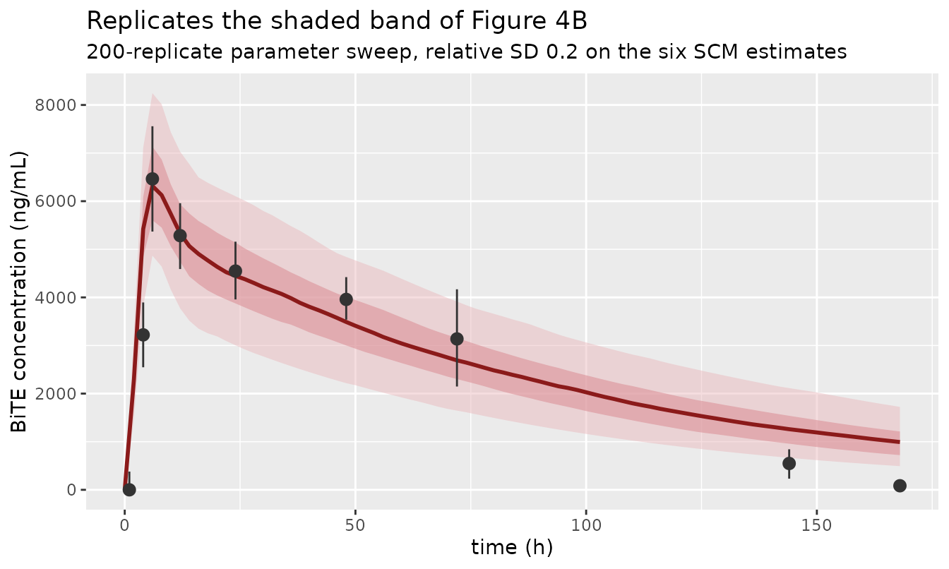
Tissue distribution
One motivation for a whole-body model is predicting exposure the experiment never measured. The liver interstitium is where translation happens, so it carries by far the highest BiTE concentration.
# The observation grid starts at 1 h so the log-scale panel has no zero record;
# this is a plotting choice and is unrelated to the PKNCA input above.
ev_t <- rxode2::et(amt = DOSE_UG(1.5), cmt = "mrna_plasma", time = 0) |>
  rxode2::et(time = seq(1, 168, by = 1), cmt = "plasma")
sim_t <- rxode2::rxSolve(scm, ev_t, returnType = "data.frame", useLinCmt = FALSE)

tissue <- tibble::tibble(
  time = sim_t$time,
  `Plasma`             = sim_t$plasma / 0.00094435,
  `Liver interstitium` = sim_t$is_liver / 3.84595163e-04,
  `Tumour interstitium`= sim_t$is_tumor / (0.55 * 0.000472),
  `Muscle interstitium`= sim_t$is_muscle / 1.47147e-03
) |>
  tidyr::pivot_longer(-time, names_to = "space", values_to = "conc")

ggplot(tissue, aes(time, conc, colour = space)) +
  geom_line(linewidth = 0.9) +
  scale_y_log10() +
  labs(x = "time (h)", y = "BiTE concentration (ng/mL, log scale)", colour = NULL,
       title = "Predicted BiTE distribution after 1.5 mg/kg mRNA-BiTE (SCM)")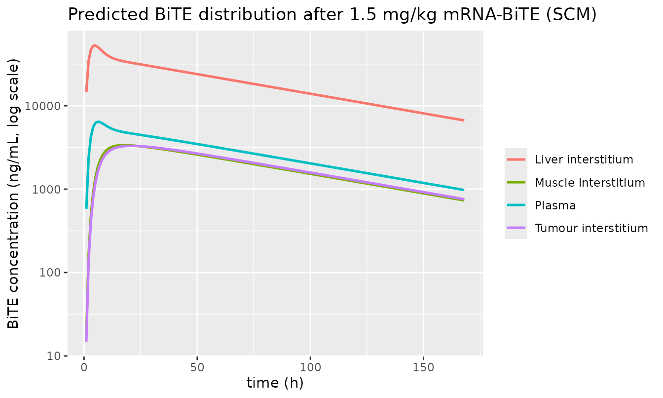
peak <- tissue |> dplyr::group_by(space) |> dplyr::summarise(peak = max(conc))
stopifnot(
  # translation occurs in the liver interstitium, so it must lead every other space
  peak$peak[peak$space == "Liver interstitium"] == max(peak$peak),
  # the paper's own caveat: tissue predictions are unvalidated, but must be finite
  all(is.finite(peak$peak))
)
knitr::kable(peak |> dplyr::arrange(dplyr::desc(peak)) |>
               dplyr::mutate(peak = signif(peak, 4)) |>
dplyr::rename("Space" = space, "Peak concentration (ng/mL)" = peak))| Space | Peak concentration (ng/mL) |
|---|---|
| Liver interstitium | 52690 |
| Plasma | 6427 |
| Muscle interstitium | 3363 |
| Tumour interstitium | 3300 |
As the authors note in the Discussion, these tissue predictions are a capability of the platform, not a validated output: the only quantitative data available are plasma profiles, so “additional concentration-time profile data specific for each organ … is needed in order to validate this prediction.”
Assumptions and deviations
The authors deposited their complete MATLAB source, so almost nothing
had to be assumed. Three discrepancies between the printed paper and
that deposit were found and are resolved as follows; all three are
recorded as a comment block at the top of model() in both
files.
Two-pore convective coefficients.
Parameters_collection_BiTEs_55kDa.mdefines the osmotic reflection coefficientssigma_S = 0.906andsigma_L = 0.0877and then never references them: the convective terms of the two-pore clearance use(1 - alpha_L)and(1 - alpha_S), the fractional hydraulic conductances, where two-pore theory calls for(1 - sigma_L)and(1 - sigma_S). Because Table 1 was fitted with the deposit’s form and the published figures were generated from it, that form is reproduced here. Substituting the reflection coefficients changes the plasma profile by at most 0.2%, so the choice is immaterial to every result in the paper. The paper does not print these equations, deferring to Li and Shah (2019), which was not available when this model was built; the deposit is therefore the operative definition.Large-intestine transcapillary terms. All three of the deposit’s ODE files drive the large-intestine two-pore clearance off
C_V_HEARTinstead ofC_V_LG_INT– a copy-paste slip. The paper’s Equations 3 and 5 are written per organ, socv_lris used here. The difference on the plasma profile is below 0.03%.Printed Equations 7 and 8. As typeset, Equation 7 reads
d mRNA_LV2/dt = k_s12 mRNA_LV1 - k_s23 mRNA_LV1 - k_d mRNA_LV2and Equation 8 readsd mRNA_LV3/dt = k_s23 mRNA_LV2 - k_d mRNA_LV2. Both subscripts are wrong: as printed, the transfer out of state 2 would not depend on state 2, and state 3 would never clear. Mass balance and the deposit (LCM.mlines 279-280) both give- k_s23 mRNA_LV2and- k_d mRNA_LV3, which is what is implemented.
Further notes:
-
CL_updiffers 100-fold between the two variants. The Table 1 footnote states thatCL_up“has been estimated using the PK data of the recombinant version of the product”, which is the same dataset for both variants, yet the table reports 1e-1 for the SCM and 1e-3 for the LCM. The depositedLCM_parameters_estimated.matconfirms 9.9996e-4, so the values are reproduced as published. In practice this means the LCM’s protein-transport module is not interchangeable with the SCM’s: dosingplasmain the LCM file does not reproduce Figure 4A. UseFiandaca_2025_mRNABiTE_scmfor the recombinant arm. - Tumour lymph is not returned to the lymph node. The deposit’s lymph-node equation sums the 15 anatomical tissues but omits the tumour’s interstitial lymph flow, a small mass-balance leak. Reproduced as written.
-
No random effects and no residual error. Neither
the paper nor the deposit reports a between-subject variance or a
residual-error magnitude; the model is fitted by least squares on
relative deviations and simulated deterministically.
propSdis therefore carried asfixed(0)and the published uncertainty bands are reproduced above as an explicit parameter sweep, which is what Materials and methods describes. - Body weight. The physiological parameter set is a 0.028 kg mouse while the deposit’s dose arithmetic uses 0.02 kg. Both are carried through unchanged because the 0.02 kg figure is what reproduces the absolute doses (120 ug and 30 ug) that Huang et al. report.
-
Local, not global, identifiability. The authors’
GenSSI analysis established only local structural identifiability, and
they “refrain from discussing the estimated values of rates”. The
individual mRNA-state rates should be read as a phenomenological delay
description, not as measured biology; that is why the liver mRNA chain
is declared through
paper_specific_compartmentsrather than mapped onto canonical compartment roles. - Upstream platform. Li and Shah (2019) was not available when this model was built. It was not needed: the authors’ deposit supplies every physiological constant, every size-dependent two-pore constant and every equation in executable form, and each is traced to the deposit line in the model files.