Monoclonal antibody TMDD model instability (Duffull 2025)

Model and source

Duffull 2025 is a tutorial on diagnosing and resolving population-model instability. Its case example 1 works through a two-compartment target-mediated drug disposition (TMDD) model for an unnamed monoclonal antibody (mAb), shows that the quasi-steady-state binding constant is not deterministically identifiable under a realistic clinical sampling design, and resolves the instability by simplifying the model in the target-saturated limit. Both the unstable full model and the stable simplification are packaged here, because the pair is what makes the tutorial’s argument reproducible.

• Citation: Duffull SB, Wright DFB, Zhu X, Liu X, Abulfathi A, Hishe H. A pharmacometric workflow for resolving model instability in model use-reuse settings. CPT Pharmacometrics Syst Pharmacol. 2025;14(10):1547-1556. doi:10.1002/psp4.70049
• Article: https://doi.org/10.1002/psp4.70049

Full model (Duffull_2025_mab_tmdd_qss) – Two-compartment target-mediated drug disposition (TMDD) model with quasi-steady-state target binding confined to the central compartment, for an unnamed monoclonal antibody (mAb) and its soluble target; case example 1 of the Duffull 2025 model-instability tutorial (Equations 1-3; Table 2 ‘Nominal value’ column). Free antibody exchanges with a peripheral compartment by first-order rate constants and is removed both by linear clearance and by saturable target-mediated internalisation of the antibody-target complex. The total target (free target plus antibody-target complex) is a dynamic state with zero-order synthesis and first-order degradation, initialised at its drug-free steady state ksyn*Vc/kdeg. Cc is the free antibody concentration and Ctotal_target is the total target concentration, both nmol/L. This is the FULL model that the tutorial shows to be structurally identifiable under a rich design but NOT deterministically identifiable under the reduced clinical design (Km relative standard error 1495.65%); the target-saturated simplification that the authors adopted instead is packaged separately as Duffull_2025_mab_tmdd_simplified. Parameter values are the nominal set used for the Fisher-information evaluations, not a fit to observed patient data: the tutorial’s datasets were generated under the stated sampling designs.

Simplified model (Duffull_2025_mab_tmdd_simplified) – Two-compartment TMDD model for an unnamed monoclonal antibody (mAb) simplified under the target-saturated limit, and the model the Duffull 2025 tutorial adopted to resolve the instability of its full counterpart (Equations 2, 4 and 5; Table 2 ‘Simplified model’ column). Because the free-antibody amount in the central compartment exceeds KmVc by roughly two orders of magnitude over the 24 h observation window, the binding saturation fraction LC/(LC + KmVc) is set to 1: the binding constant Km drops out of the model entirely and target-mediated removal of antibody becomes kintRtot, independent of antibody amount. The total target still has zero-order synthesis and first-order internalisation, and kdeg survives only through the drug-free initial condition ksynVc/kdeg. Cc is the free antibody concentration and Ctotal_target is the total target concentration, both nmol/L. All parameters were estimated with relative standard errors below 30% under the reduced clinical sampling design that made the full model unidentifiable. IMPORTANT: this approximation is valid only while the target remains saturated – it makes target-mediated antibody removal a constant-rate sink, so the free-antibody state can be driven negative once antibody washes out. Restrict simulations to the 24 h window the source validated. The full model is packaged as Duffull_2025_mab_tmdd_qss.

What this paper is, and what is not packaged

This is a methods tutorial, not a drug-development report, and only part of it yields a packageable model. For the reviewer’s benefit:

• Case example 1 (TMDD, packaged as the two models above). Equations 1-3 give the full model and Equations 2, 4 and 5 the simplification; Table 2 gives a complete parameter set for each. Fully specified, so fully extracted.
• Case example 2 (allopurinol / oxypurinol turnover PKPD, NOT packaged). Section 2.2 fits a urate turnover model to 648 patients and concludes that it is not internally deterministically identifiable, because oxypurinol’s elimination rate constant and urate’s turnover rate constant are too close to separate. The resolution the authors adopt in Section 2.2.5 is “to simplify the model structure using an immediate effects PD model” – which is exactly the model already in this library as Wright_2016_allopurinol, co-authored by this paper’s first two authors. The turnover variant is therefore both superseded and explicitly reported as unreliable (Table 3: kout relative standard error 125%, between-subject variability on kout 257 CV% with its own RSE 239%). Two further gaps make it unpackageable as it stands: the oxypurinol PK is fixed to individual empirical Bayes estimates (“IPP”) rather than a reported population PK model, so there is no PK layer in the paper; and Table 3’s theta diuretic = 1.7 is given as a “fractional effect of diuretic” without saying which parameter it acts on.
• The stochastic simulation-estimation scenario in Section 2.2.4 (NOT packaged). A hypothetical one-compartment PK plus turnover PD model used to demonstrate the ke vs kout flip. It reports ke, three kout settings and residual-error magnitudes, but not Emax, ka, V or Rin, so it cannot be assembled without inventing values.

Population

The source is a tutorial, so the “population” is thin by design and is recorded honestly rather than embellished. Case example 1 used 80 subjects given a single intravenous bolus into the central compartment, with free antibody and total target (free target plus antibody-target complex) both measured. Neither the antibody nor its target is named, and no demographics, age, weight, sex or region are reported. The species is never stated; the framing (“sparse sampling, common in mAb clinical trials”) implies human.

Two sampling designs are used (Section 2.1.3):

Design	Sampling times (h post-dose)	Free drug obs	Total target obs
Hypothetical rich (structural identifiability template)	0, 0.01, 0.2, 0.6, 3, 50, 64, 81, 91	640	720
Reduced clinical (deterministic identifiability, and the simplified model’s estimation design)	0, 0.5, 3, 5, 12, 24	400	480

The datasets are simulated, not observed: the reported observation counts are exactly the sampling grids multiplied by 80 subjects (80 x 9 = 720 and 80 x 6 = 480 total target; the free-drug counts are one time point fewer, 80 x 8 = 640 and 80 x 5 = 400).

The same information is available programmatically via readModelDb("Duffull_2025_mab_tmdd_qss")()$population.

Source trace

Per-parameter origins are also recorded as in-file comments beside each ini() entry in inst/modeldb/pharmacokinetics/Duffull_2025_mab_tmdd_qss.R and ..._simplified.R.

Equations

Model element	Encoded as	Source location
dLC/dt = -(ke + k12) LC + k21 LT - kint LC Rtot / (LC + Km Vc)	d/dt(central), full model	Duffull 2025 Equation 1, p. 1551
dLT/dt = k12 LC - k21 LT	d/dt(peripheral1), both models	Duffull 2025 Equation 2, p. 1551
dRtot/dt = -(kint - kdeg) LC Rtot / (LC + Km Vc) - kdeg Rtot + ksyn Vc	d/dt(total_target), full model	Duffull 2025 Equation 3, p. 1551
dLC/dt = -(ke + k12) LC + k21 LT - kint Rtot	d/dt(central), simplified model	Duffull 2025 Equation 4, p. 1551
dRtot/dt = -kint Rtot + ksyn VC	d/dt(total_target), simplified model	Duffull 2025 Equation 5, p. 1551
LC(0) = 0, LT(0) = 0, Rtot(0) = ksyn VC / kdeg	state initial conditions	Duffull 2025, stated below Equation 5, p. 1551
ke = CL/Vc, k12 = Q/Vc, k21 = Q/Vp	micro-constants in model()	Derived: the equations are written in rate constants but Table 2 tabulates CL, Vc, Vp, Q
Two compartments, single IV bolus into central, binding in central only	model structure	Duffull 2025 Section 2.1.5, p. 1551
Outputs: free drug concentration, total target concentration	Cc, Ctotal_target	Duffull 2025 Section 2.1.1, p. 1550

Parameters

Full is the Table 2 “Nominal value” column (the parameter set at which the Fisher information matrix was evaluated); Simplified is the Table 2 “Simplified model” column (final estimates, RSE in parentheses).

Parameter	Full	Simplified	Source location
lcl (CL, L/h)	4.13	4.15 (6%)	Duffull 2025 Table 2 row CL
lvc (Vc, L)	76.7	68.4 (9%)	Duffull 2025 Table 2 row Vc
lvp (Vp, L)	70	75.8 (5%)	Duffull 2025 Table 2 row Vp
lq (Q, L/h)	44.7	59.9 (11%)	Duffull 2025 Table 2 row Q
lksyn (ksyn, nmol/L/h)	1.09	1.16 (6%)	Duffull 2025 Table 2 row ksyn
lkdeg (kdeg, 1/h)	0.349	0.373 (4%)	Duffull 2025 Table 2 row kdeg
lkint (kint, 1/h)	11.1	11.5 (5%)	Duffull 2025 Table 2 row kint
lkss (Km in the source; Kss, nmol/L)	0.13	absent	Duffull 2025 Table 2 row Km (dash in the simplified column)
etalcl (IIV CL, CV%)	25	21.9 (15%)	Duffull 2025 Table 2 row IIV-CL
etalvc (IIV Vc, CV%)	25	31.1 (17%)	Duffull 2025 Table 2 row IIV-Vc
etalksyn (IIV ksyn, CV%)	25	32.6 (14%)	Duffull 2025 Table 2 row IIV-ksyn
etalkint (IIV kint, CV%)	25	28.7 (13%)	Duffull 2025 Table 2 row IIV-kint
propSd, propSd_Ctotal_target	fixed(0)	fixed(0)	Not reported by the source (see Assumptions)
Dose = 10000 nmol IV bolus	vignette event table	Read off Duffull 2025 Figure 3 (free-drug amount at t = 0); not stated in the text

Two naming translations were applied, both to existing canonicals:

• The source’s Km is recorded as lkss. Its role in Equations 1 and 3 is the quasi-steady-state binding constant of the Gibiansky 2008 TMDD reduction (it scales free-drug saturation of target-mediated internalisation while the total target remains a dynamic state), which is what this library’s PK_2cmt_tmdd_qss archetype calls lkss. It is not a metabolic Michaelis-Menten constant (canonical lkm), which would describe saturable elimination with no target state.
• The source’s Rtot state is the canonical compartment total_target, and its concentration output is Ctotal_target.

mod_full <- readModelDb("Duffull_2025_mab_tmdd_qss")
mod_simp <- readModelDb("Duffull_2025_mab_tmdd_simplified")

DOSE  <- 10000  # nmol; read off Figure 3
TOBS  <- c(0, 0.5, 3, 5, 12, 24)  # reduced clinical design, Section 2.1.3

# Event-table helper. Both models expose two `~` endpoints (Cc and
# Ctotal_target), so observation rows must carry `dvid` rather than a `cmt`
# naming an algebraic observable; rxode2 returns BOTH observable columns at
# every observation row regardless.
make_events <- function(n, times, id_offset = 0L) {
  ids <- id_offset + seq_len(n)
  dplyr::bind_rows(
    tibble(id = ids, time = 0, amt = DOSE, evid = 1L,
           cmt = "central", dvid = NA_integer_),
    tidyr::expand_grid(id = ids, time = times) |>
      mutate(amt = NA_real_, evid = 0L, cmt = NA_character_, dvid = 1L)
  ) |>
    arrange(id, time, desc(evid))
}

Structural verification

Three checks establish that the packaged ODEs are the source’s ODEs, before any attempt to reproduce a figure. They are the gates that a visual profile comparison would not catch.

The simplification is algebraically exact in the saturated limit

Duffull 2025 derives Equations 4 and 5 by setting the saturation fraction LC/(LC + Km*Vc) to 1. That substitution should be exact, and in the target equation the kdeg terms should cancel:

-(kint - kdeg) Rtot - kdeg Rtot + ksyn Vc = -kint Rtot + ksyn Vc

So driving Kss to zero in the full model must reproduce the simplified model run with the same parameters, to solver precision. If the transcription of either equation set were wrong, this would not hold.

ev1 <- make_events(1, seq(0, 24, by = 0.05))
full_pars <- c(lcl = log(4.13), lvc = log(76.7), lvp = log(70), lq = log(44.7),
               lksyn = log(1.09), lkdeg = log(0.349), lkint = log(11.1))

sat_limit <- rxSolve(zeroRe(mod_full), ev1,
                     params = c(full_pars, lkss = log(0.13 * 1e-6)),
                     returnType = "data.frame")
#> ℹ parameter labels from comments will be replaced by 'label()'
#> ℹ omega/sigma items treated as zero: 'etalcl', 'etalvc', 'etalksyn', 'etalkint'
simp_same <- rxSolve(zeroRe(mod_simp), ev1, params = full_pars,
                     returnType = "data.frame")
#> ℹ parameter labels from comments will be replaced by 'label()'
#> ℹ omega/sigma items treated as zero: 'etalcl', 'etalvc', 'etalksyn', 'etalkint'

rel_diff <- max(abs(simp_same$central - sat_limit$central) /
                  pmax(sat_limit$central, 1e-8))
cat(sprintf("max relative difference in free-drug amount = %.3g\n", rel_diff))
#> max relative difference in free-drug amount = 6.05e-11
stopifnot(rel_diff < 1e-6)

The target-mediated term actually reaches the integrator

In the nlmixr2 model-function form, a named intermediate referencing an ODE state can silently evaluate to zero inside d/dt(), deleting a whole elimination pathway with no error. Both models therefore write the saturation fraction inline. This exaggeration test proves the term is live: making Kss enormous switches target-mediated elimination off, which must raise exposure.

nominal <- rxSolve(zeroRe(mod_full), ev1, returnType = "data.frame")
#> ℹ parameter labels from comments will be replaced by 'label()'
#> ℹ omega/sigma items treated as zero: 'etalcl', 'etalvc', 'etalksyn', 'etalkint'
inert   <- rxSolve(zeroRe(mod_full), ev1,
                   params = c(lkss = log(0.13 * 1e6)), returnType = "data.frame")
#> ℹ parameter labels from comments will be replaced by 'label()'
#> ℹ omega/sigma items treated as zero: 'etalcl', 'etalvc', 'etalksyn', 'etalkint'

lc24_nominal <- nominal$central[nrow(nominal)]
lc24_inert   <- inert$central[nrow(inert)]
cat(sprintf("LC(24 h) with nominal Kss = %.1f nmol\n", lc24_nominal))
#> LC(24 h) with nominal Kss = 1756.1 nmol
cat(sprintf("LC(24 h) with Kss x 1e6   = %.1f nmol (target term switched off)\n", lc24_inert))
#> LC(24 h) with Kss x 1e6   = 2575.9 nmol (target term switched off)
cat(sprintf("ratio = %.3f\n", lc24_inert / lc24_nominal))
#> ratio = 1.467
stopifnot(lc24_inert / lc24_nominal > 1.05)  # term is live, not inert

Target baseline and saturated plateau

The total target must start at its drug-free steady state ksyn/kdeg and, once the antibody saturates it, fall to the plateau of Equation 5, ksyn/kint.

tt_checks <- tibble(
  Quantity = c("Baseline total target Rtot(0)/Vc",
               "Saturated plateau (Equation 5 steady state)"),
  `Closed form` = c("ksyn / kdeg", "ksyn / kint"),
  Expected = c(1.09 / 0.349, 1.09 / 11.1),
  Simulated = c(nominal$Ctotal_target[1], nominal$Ctotal_target[nrow(nominal)])
) |>
  mutate(`% diff` = 100 * (Simulated - Expected) / Expected)
knitr::kable(tt_checks, digits = 4,
             caption = "Total target concentration (nmol/L), full model, typical values.")

Total target concentration (nmol/L), full model, typical values.

Quantity	Closed form	Expected	Simulated	% diff
Baseline total target Rtot(0)/Vc	ksyn / kdeg	3.1232	3.1232	0.0000
Saturated plateau (Equation 5 steady state)	ksyn / kint	0.0982	0.0987	0.5473

stopifnot(max(abs(tt_checks$`% diff`)) < 1)

Virtual cohort

Each model is simulated as one cohort of 100 subjects on the reduced clinical design, well inside the 200-per-arm cap. Between-subject variability comes from the model’s own etalcl, etalvc, etalksyn and etalkint; there are no covariates to sample, because Duffull 2025 turns covariate effects off for the identifiability analyses and reports no covariate model.

SEED <- 20251009
N <- 100
grid_dense <- sort(unique(c(seq(0, 24, by = 0.25), TOBS)))
events <- make_events(N, grid_dense)
stopifnot(!anyDuplicated(events[events$evid == 0L, c("id", "time")]))

Simulation

The seed is reset immediately before each solve, so both models are simulated on the same draw of etalcl, etalvc, etalksyn and etalkint. That makes the full-versus-simplified comparison paired at the subject level; seeding once and solving twice would give each model a different cohort and confound the structural comparison with sampling noise.

set.seed(SEED)
sim_full <- rxSolve(mod_full, events, returnType = "data.frame") |>
  mutate(model = "Full TMDD (Eq 1-3)")
#> ℹ parameter labels from comments will be replaced by 'label()'
set.seed(SEED)
sim_simp <- rxSolve(mod_simp, events, returnType = "data.frame") |>
  mutate(model = "Simplified (Eq 2, 4, 5)")
#> ℹ parameter labels from comments will be replaced by 'label()'
sim <- bind_rows(sim_full, sim_simp) |>
  mutate(model = factor(model, levels = c("Full TMDD (Eq 1-3)",
                                          "Simplified (Eq 2, 4, 5)")))

Replicate Figure 3

Figure 3 of Duffull 2025 plots the free-drug amount in the central compartment (red) against Km * Vc (blue) over 24 h on a log scale, with 95% intervals, to justify the simplification. Both quantities carry between-subject variability here because Vc has an eta.

fig3 <- sim_full |>
  mutate(km_vc = kss * vc) |>
  group_by(time) |>
  summarise(
    drug_med = median(central), drug_lo = quantile(central, 0.025),
    drug_hi  = quantile(central, 0.975),
    km_med   = median(km_vc),   km_lo = quantile(km_vc, 0.025),
    km_hi    = quantile(km_vc, 0.975),
    .groups = "drop"
  )

ggplot(fig3, aes(x = time)) +
  geom_ribbon(aes(ymin = drug_lo, ymax = drug_hi), fill = "red", alpha = 0.15) +
  geom_line(aes(y = drug_med, colour = "Free drug in central compartment"), linewidth = 0.9) +
  geom_ribbon(aes(ymin = km_lo, ymax = km_hi), fill = "blue", alpha = 0.15) +
  geom_line(aes(y = km_med, colour = "Km * Vc"), linewidth = 0.9) +
  scale_y_log10(limits = c(1, 20000)) +
  scale_colour_manual(values = c("Free drug in central compartment" = "red",
                                 "Km * Vc" = "blue")) +
  labs(x = "Time (h)", y = "Amount (nmol)", colour = NULL) +
  theme_bw() + theme(legend.position = "top")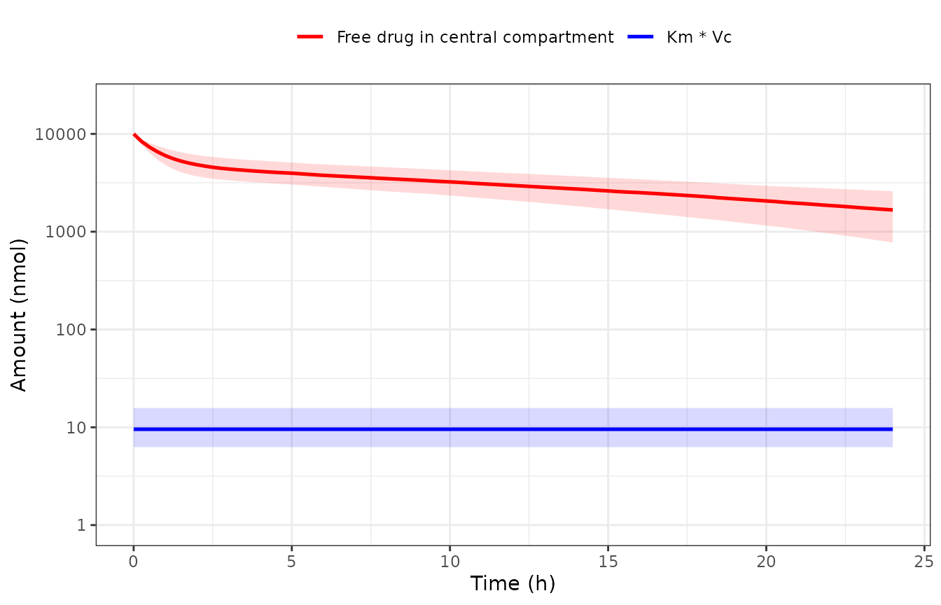

Replicates Figure 3 of Duffull 2025: free-drug amount in the central compartment versus Km * Vc over the first 24 h (full model). Lines are medians, ribbons 95% intervals.

The source’s justification is that “during the first 24 h, the drug amount in the central compartment exceeded the Km x VC value by almost 100 fold”. Checked against the median profile that Figure 3 draws, the margin holds with room to spare – but the cohort tail is worth reporting, because the approximation is a per-subject claim and the paper’s figure only shows the aggregate:

ratios <- sim_full |>
  filter(time > 0) |>
  mutate(ratio = central / (kss * vc))

median_margin <- ratios |>
  group_by(time) |>
  summarise(m = median(central) / median(kss * vc), .groups = "drop") |>
  pull(m) |>
  min()

per_subject_min <- ratios |>
  group_by(id) |>
  summarise(mn = min(ratio), .groups = "drop")

cat(sprintf("median-profile minimum free-drug / (Km * Vc) over 0-24 h = %.1f\n",
            median_margin))
#> median-profile minimum free-drug / (Km * Vc) over 0-24 h = 174.7
cat(sprintf("per-subject minima: median %.1f, 2.5th percentile %.1f, lowest %.1f\n",
            median(per_subject_min$mn), quantile(per_subject_min$mn, 0.025),
            min(per_subject_min$mn)))
#> per-subject minima: median 174.2, 2.5th percentile 78.0, lowest 40.6
cat(sprintf("subjects dipping below 100-fold at some point: %d of %d\n",
            sum(per_subject_min$mn < 100), nrow(per_subject_min)))
#> subjects dipping below 100-fold at some point: 6 of 100
stopifnot(median_margin > 100)  # the source's claim, on the profile it plots

So the source’s stated margin is a property of the typical profile. With the published 25% CV on CL and Vc, a minority of subjects (6 of 100 at this seed) spend part of the window under a 100-fold margin, where the saturated approximation is correspondingly weaker. That is consistent with – and slightly sharpens – the tutorial’s argument: the simplification is justified on the aggregate design, and the residual error it introduces is concentrated in the tail.

Quantitative gates against closed-form identities

The source reports no NCA table, so there is nothing to transcribe for a side-by-side comparison. Closed-form identities are used instead, and they are the stronger check: each one gates the ODE encoding, the dose encoding, the observation scaling and the NCA settings simultaneously.

Cmax equals dose / Vc

An IV bolus into the central compartment must peak at dose / Vc exactly.

cmax_gate <- tibble(
  model = c("Full TMDD (Eq 1-3)", "Simplified (Eq 2, 4, 5)"),
  Vc = c(76.7, 68.4),
  Expected = DOSE / Vc,
  Simulated = c(
    rxSolve(zeroRe(mod_full), ev1, returnType = "data.frame")$Cc[1],
    rxSolve(zeroRe(mod_simp), ev1, returnType = "data.frame")$Cc[1]
  )
) |>
  mutate(`% diff` = 100 * (Simulated - Expected) / Expected)
#> ℹ parameter labels from comments will be replaced by 'label()'
#> ℹ omega/sigma items treated as zero: 'etalcl', 'etalvc', 'etalksyn', 'etalkint'
#> ℹ parameter labels from comments will be replaced by 'label()'
#> ℹ omega/sigma items treated as zero: 'etalcl', 'etalvc', 'etalksyn', 'etalkint'
knitr::kable(cmax_gate, digits = 4,
             caption = "Cmax of free antibody (nmol/L), typical values.")

Cmax of free antibody (nmol/L), typical values.

model	Vc	Expected	Simulated	% diff
Full TMDD (Eq 1-3)	76.7	130.3781	130.3781	0
Simplified (Eq 2, 4, 5)	68.4	146.1988	146.1988	0

stopifnot(max(abs(cmax_gate$`% diff`)) < 1e-6)

PKNCA instrument gate: AUC0-inf equals dose / CL for the linear reduction

Setting ksyn to zero removes the target entirely (Rtot(0) = ksyn*Vc/kdeg and the synthesis term both vanish), so each model collapses to a plain linear two-compartment IV bolus, for which AUC0-inf = dose / CL and the terminal half-life is ln(2) over the smaller eigenvalue of the disposition matrix. Reproducing both through PKNCA confirms the NCA machinery is set up correctly before it is used on the target-mediated model.

ev_long <- make_events(1, sort(unique(c(seq(0, 48, by = 0.25),
                                       seq(48, 336, by = 2)))))

lin_profile <- function(mod) {
  rxSolve(zeroRe(mod), ev_long, params = c(lksyn = log(1e-12)),
          returnType = "data.frame")
}

nca_of <- function(df, intervals) {
  conc <- df |> filter(!is.na(Cc)) |> transmute(id = 1L, time, Cc)
  dose <- tibble(id = 1L, time = 0, amt = DOSE)
  PKNCA::pk.nca(PKNCA::PKNCAdata(
    PKNCA::PKNCAconc(conc, Cc ~ time | id, concu = "nmol/L", timeu = "h"),
    PKNCA::PKNCAdose(dose, amt ~ time | id, doseu = "nmol"),
    intervals = intervals
  ))
}

lin_intervals <- data.frame(start = 0, end = Inf,
                            cmax = TRUE, aucinf.obs = TRUE, half.life = TRUE)

# Analytic terminal half-life of the linear reduction.
analytic_thalf <- function(cl, vc, vp, q) {
  ke <- cl / vc; k12 <- q / vc; k21 <- q / vp
  s <- ke + k12 + k21
  lam2 <- (s - sqrt(s^2 - 4 * ke * k21)) / 2
  log(2) / lam2
}

lin_gate <- bind_rows(
  lapply(
    list(list(nm = "Full TMDD (Eq 1-3)",      mod = mod_full,
              cl = 4.13, vc = 76.7, vp = 70,   q = 44.7),
         list(nm = "Simplified (Eq 2, 4, 5)", mod = mod_simp,
              cl = 4.15, vc = 68.4, vp = 75.8, q = 59.9)),
    function(z) {
      res <- as.data.frame(nca_of(lin_profile(z$mod), lin_intervals)$result)
      getp <- function(p) res$PPORRES[res$PPTESTCD == p][1]
      tibble(
        model = z$nm,
        `AUC0-inf expected (dose/CL)` = DOSE / z$cl,
        `AUC0-inf PKNCA` = getp("aucinf.obs"),
        `t1/2 expected (eigenvalue)` = analytic_thalf(z$cl, z$vc, z$vp, z$q),
        `t1/2 PKNCA` = getp("half.life")
      )
    }
  )
) |>
  mutate(`AUC % diff` = 100 * (`AUC0-inf PKNCA` - `AUC0-inf expected (dose/CL)`) /
           `AUC0-inf expected (dose/CL)`,
         `t1/2 % diff` = 100 * (`t1/2 PKNCA` - `t1/2 expected (eigenvalue)`) /
           `t1/2 expected (eigenvalue)`)
#> ℹ parameter labels from comments will be replaced by 'label()'
#> ℹ omega/sigma items treated as zero: 'etalcl', 'etalvc', 'etalksyn', 'etalkint'
#> ℹ parameter labels from comments will be replaced by 'label()'
#> ℹ omega/sigma items treated as zero: 'etalcl', 'etalvc', 'etalksyn', 'etalkint'

knitr::kable(lin_gate, digits = 3,
             caption = "Linear reduction (ksyn -> 0): PKNCA versus closed form. AUC in nmol*h/L, half-life in h.")

Linear reduction (ksyn -> 0): PKNCA versus closed form. AUC in nmol*h/L, half-life in h.

model	AUC0-inf expected (dose/CL)	AUC0-inf PKNCA	t1/2 expected (eigenvalue)	t1/2 PKNCA	AUC % diff	t1/2 % diff
Full TMDD (Eq 1-3)	2421.308	2421.585	25.151	25.124	0.011	-0.107
Simplified (Eq 2, 4, 5)	2409.639	2410.083	24.554	24.531	0.018	-0.092

stopifnot(max(abs(lin_gate$`AUC % diff`))  < 0.5)
stopifnot(max(abs(lin_gate$`t1/2 % diff`)) < 2)

PKNCA: AUC0-24 of the target-mediated models

AUC24h is the source’s own response index – it is what the Sobol global sensitivity analysis of Figure 2 attributes variance to – so it is the natural exposure metric to summarise. The interval ends at 24 h, which is both the reduced design’s last sampling time and the window over which the target-saturated approximation was justified.

nca_cohort <- function(df, conc_col) {
  conc <- df |>
    filter(!is.na(.data[[conc_col]])) |>
    transmute(id, model, conc = .data[[conc_col]], time)
  dose <- events |>
    filter(evid == 1L) |>
    transmute(id, time, amt) |>
    tidyr::expand_grid(model = unique(df$model)) |>
    select(id, model, time, amt)
  PKNCA::pk.nca(PKNCA::PKNCAdata(
    PKNCA::PKNCAconc(conc, conc ~ time | model + id,
                     concu = "nmol/L", timeu = "h"),
    PKNCA::PKNCAdose(dose, amt ~ time | model + id, doseu = "nmol"),
    intervals = data.frame(start = 0, end = 24,
                           cmax = TRUE, tmax = TRUE, auclast = TRUE)
  ))
}

nca_drug   <- nca_cohort(sim, "Cc")
nca_target <- nca_cohort(sim, "Ctotal_target")

summarise_nca <- function(res, label) {
  as.data.frame(res$result) |>
    filter(PPTESTCD %in% c("cmax", "tmax", "auclast")) |>
    group_by(model, PPTESTCD) |>
    summarise(median = median(PPORRES, na.rm = TRUE),
              p2.5 = quantile(PPORRES, 0.025, na.rm = TRUE),
              p97.5 = quantile(PPORRES, 0.975, na.rm = TRUE), .groups = "drop") |>
    mutate(Analyte = label)
}

nca_tbl <- bind_rows(summarise_nca(nca_drug, "Free antibody (Cc)"),
                     summarise_nca(nca_target, "Total target (Ctotal_target)")) |>
  mutate(Parameter = recode(PPTESTCD,
                            cmax = "Cmax (nmol/L)", tmax = "Tmax (h)",
                            auclast = "AUC0-24 (nmol*h/L)")) |>
  select(Analyte, Parameter, model, median, p2.5, p97.5) |>
  rename("Model" = model, "Median" = median,
         "2.5th pct" = p2.5, "97.5th pct" = p97.5) |>
  arrange(Analyte, Parameter, Model)

knitr::kable(nca_tbl, digits = 3,
             caption = "PKNCA summary over 0-24 h, 100 simulated subjects per model.")

PKNCA summary over 0-24 h, 100 simulated subjects per model.

Analyte	Parameter	Model	Median	2.5th pct	97.5th pct
Free antibody (Cc)	AUC0-24 (nmol*h/L)	Full TMDD (Eq 1-3)	1032.167	759.320	1344.296
Free antibody (Cc)	AUC0-24 (nmol*h/L)	Simplified (Eq 2, 4, 5)	1052.803	716.376	1389.621
Free antibody (Cc)	Cmax (nmol/L)	Full TMDD (Eq 1-3)	136.153	82.982	207.575
Free antibody (Cc)	Cmax (nmol/L)	Simplified (Eq 2, 4, 5)	154.297	83.399	260.746
Free antibody (Cc)	Tmax (h)	Full TMDD (Eq 1-3)	0.000	0.000	0.000
Free antibody (Cc)	Tmax (h)	Simplified (Eq 2, 4, 5)	0.000	0.000	0.000
Total target (Ctotal_target)	AUC0-24 (nmol*h/L)	Full TMDD (Eq 1-3)	2.582	1.425	4.687
Total target (Ctotal_target)	AUC0-24 (nmol*h/L)	Simplified (Eq 2, 4, 5)	2.628	1.227	5.558
Total target (Ctotal_target)	Cmax (nmol/L)	Full TMDD (Eq 1-3)	3.019	1.891	4.818
Total target (Ctotal_target)	Cmax (nmol/L)	Simplified (Eq 2, 4, 5)	2.976	1.616	5.474
Total target (Ctotal_target)	Tmax (h)	Full TMDD (Eq 1-3)	0.000	0.000	0.000
Total target (Ctotal_target)	Tmax (h)	Simplified (Eq 2, 4, 5)	0.000	0.000	0.000

The simplification reproduces the full model over 24 h

This is the tutorial’s substantive claim: the simplified model is a usable stand-in over the observed window. Comparing typical-value profiles with each model’s own published parameters (so the comparison includes the re-estimation, not just the structural change):

tv_full <- rxSolve(zeroRe(mod_full), ev1, returnType = "data.frame")
#> ℹ parameter labels from comments will be replaced by 'label()'
#> ℹ omega/sigma items treated as zero: 'etalcl', 'etalvc', 'etalksyn', 'etalkint'
tv_simp <- rxSolve(zeroRe(mod_simp), ev1, returnType = "data.frame")
#> ℹ parameter labels from comments will be replaced by 'label()'
#> ℹ omega/sigma items treated as zero: 'etalcl', 'etalvc', 'etalksyn', 'etalkint'

cmp <- tibble(
  `Time (h)` = TOBS,
  `Full Cc (nmol/L)` = approx(tv_full$time, tv_full$Cc, TOBS)$y,
  `Simplified Cc (nmol/L)` = approx(tv_simp$time, tv_simp$Cc, TOBS)$y
) |>
  mutate(`% diff` = 100 * (`Simplified Cc (nmol/L)` - `Full Cc (nmol/L)`) /
           `Full Cc (nmol/L)`)
knitr::kable(cmp, digits = 3,
             caption = "Typical-value free-antibody concentration, each model with its own Table 2 parameters.")

Typical-value free-antibody concentration, each model with its own Table 2 parameters.

Time (h)	Full Cc (nmol/L)	Simplified Cc (nmol/L)	% diff
0.0	130.378	146.199	12.135
0.5	96.407	97.129	0.749
3.0	58.217	58.605	0.666
5.0	52.704	53.903	2.276
12.0	39.803	40.796	2.496
24.0	22.896	23.580	2.990

auc24 <- function(df) {
  d <- df[df$time <= 24, ]
  sum(diff(d$time) * (head(d$Cc, -1) + tail(d$Cc, -1)) / 2)
}
auc_pct <- 100 * (auc24(tv_simp) - auc24(tv_full)) / auc24(tv_full)

cat(sprintf("post-dose sampling times (t > 0): max |%% diff| = %.2f%%\n",
            max(abs(cmp$`% diff`[cmp$`Time (h)` > 0]))))
#> post-dose sampling times (t > 0): max |% diff| = 2.99%
cat(sprintf("AUC0-24 of the typical profile:   %% diff = %.2f%%\n", auc_pct))
#> AUC0-24 of the typical profile:   % diff = 1.92%
stopifnot(max(abs(cmp$`% diff`[cmp$`Time (h)` > 0])) < 5)
stopifnot(abs(auc_pct) < 5)

The one large entry is at t = 0, and it is not a structural discrepancy – the simplification was already shown above to be algebraically exact. An IV bolus starts at dose / Vc, so the t = 0 difference must be exactly the ratio of the two re-estimated central volumes (76.7 L versus 68.4 L). Checking that closes the loop:

t0_observed <- cmp$`% diff`[cmp$`Time (h)` == 0]
t0_expected <- 100 * (76.7 / 68.4 - 1)
cat(sprintf("t = 0 difference observed = %.4f%%, expected from Vc ratio = %.4f%%\n",
            t0_observed, t0_expected))
#> t = 0 difference observed = 12.1345%, expected from Vc ratio = 12.1345%
stopifnot(abs(t0_observed - t0_expected) < 1e-6)

So over the observed window the two models agree to within 3% at every post-dose sampling time and to within 2% on AUC0-24, with the remaining difference attributable to re-estimation of the disposition parameters rather than to the structural change. That is the tutorial’s claim, reproduced.

sim |>
  select(id, time, model, Cc, Ctotal_target) |>
  pivot_longer(c(Cc, Ctotal_target), names_to = "output", values_to = "conc") |>
  mutate(output = recode(output, Cc = "Free antibody",
                         Ctotal_target = "Total target")) |>
  group_by(model, output, time) |>
  summarise(med = median(conc), lo = quantile(conc, 0.025),
            hi = quantile(conc, 0.975), .groups = "drop") |>
  ggplot(aes(time, med, colour = model, fill = model)) +
  geom_ribbon(aes(ymin = lo, ymax = hi), alpha = 0.15, colour = NA) +
  geom_line(linewidth = 0.9) +
  facet_wrap(~output, scales = "free_y") +
  labs(x = "Time (h)", y = "Concentration (nmol/L)", colour = NULL, fill = NULL) +
  theme_bw() + theme(legend.position = "top")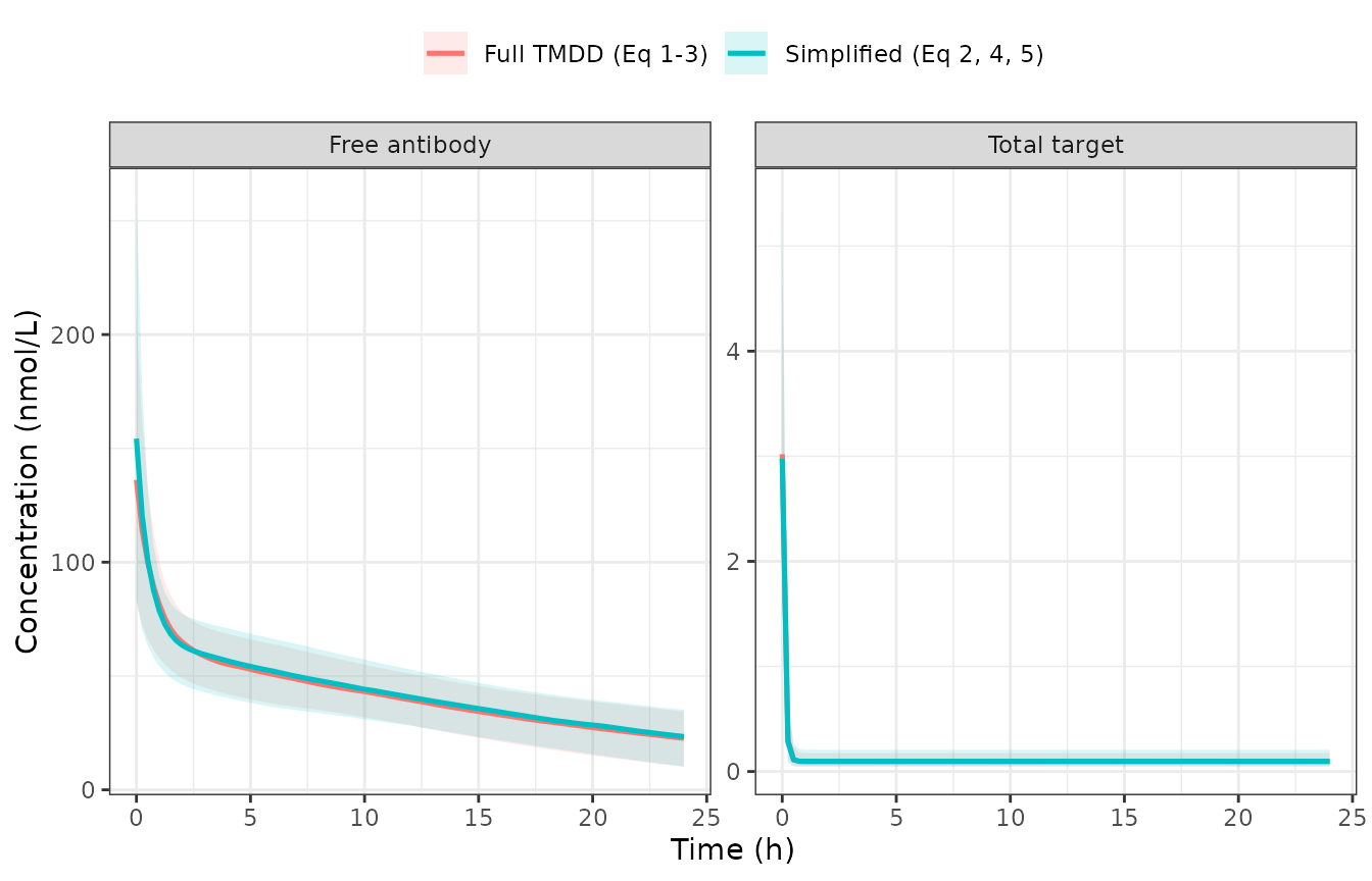

Free antibody (left) and total target (right) over 24 h: full versus simplified model. Lines are medians of 100 subjects, ribbons 95% intervals.

Limitation of the target-saturated approximation

Setting the saturation fraction to 1 makes target-mediated removal of antibody kint * Rtot, which is independent of how much antibody is present. Once Rtot reaches its plateau this is a constant-rate sink, so the free-antibody state is driven negative when antibody washes out. The full model does not have this problem, because its saturation fraction goes to zero along with the drug.

This is why the simplified model must not be simulated beyond the window the source validated.

ev_96 <- make_events(1, seq(0, 96, by = 0.25))
tail_simp <- rxSolve(zeroRe(mod_simp), ev_96, returnType = "data.frame")
#> ℹ parameter labels from comments will be replaced by 'label()'
#> ℹ omega/sigma items treated as zero: 'etalcl', 'etalvc', 'etalksyn', 'etalkint'
tail_full <- rxSolve(zeroRe(mod_full), ev_96, returnType = "data.frame")
#> ℹ parameter labels from comments will be replaced by 'label()'
#> ℹ omega/sigma items treated as zero: 'etalcl', 'etalvc', 'etalksyn', 'etalkint'

first_neg <- tail_simp$time[which(tail_simp$central < 0)][1]
cat(sprintf("simplified model: free-drug amount first goes negative at %.1f h\n", first_neg))
#> simplified model: free-drug amount first goes negative at 52.5 h
cat(sprintf("simplified model: free-drug amount at 96 h = %.1f nmol\n",
            tail_simp$central[nrow(tail_simp)]))
#> simplified model: free-drug amount at 96 h = -925.1 nmol
cat(sprintf("full model:       free-drug amount at 96 h = %.3f nmol (stays non-negative)\n",
            tail_full$central[nrow(tail_full)]))
#> full model:       free-drug amount at 96 h = 0.000 nmol (stays non-negative)
stopifnot(first_neg > 24)                             # 24 h window is safe
stopifnot(min(tail_full$central) >= -1e-6)            # full model does not

Within the 24 h window the same mechanism can still bite for subjects in the upper tail of ksyn and kint, where the constant sink is largest. Whether any subject is affected depends on the eta draw, so it is demonstrated across several seeds rather than left to chance. It is not a solver artifact: the minima are reproduced to five significant figures at atol = rtol = 1e-12.

neg_scan <- bind_rows(lapply(c(1, 3, 42, 777, SEED), function(sd) {
  bind_rows(lapply(list(list(nm = "Full TMDD (Eq 1-3)", m = mod_full),
                        list(nm = "Simplified (Eq 2, 4, 5)", m = mod_simp)),
    function(z) {
      set.seed(sd); d  <- rxSolve(z$m, events, returnType = "data.frame")
      set.seed(sd); dt <- rxSolve(z$m, events, returnType = "data.frame",
                                  atol = 1e-12, rtol = 1e-12)
      tibble(Seed = sd, Model = z$nm,
             `Subjects with negative free drug` = n_distinct(d$id[d$central < 0]),
             `Minimum free drug (nmol)` = min(d$central),
             `Minimum at atol=rtol=1e-12` = min(dt$central))
    }))
}))
knitr::kable(neg_scan, digits = 3,
             caption = "Negative free-drug states within the 24 h window, 100 subjects per model per seed.")

Negative free-drug states within the 24 h window, 100 subjects per model per seed.

Seed	Model	Subjects with negative free drug	Minimum free drug (nmol)	Minimum at atol=rtol=1e-12
1	Full TMDD (Eq 1-3)	0	679.932	679.932
1	Simplified (Eq 2, 4, 5)	0	178.330	178.331
3	Full TMDD (Eq 1-3)	0	244.648	244.648
3	Simplified (Eq 2, 4, 5)	0	80.258	80.258
42	Full TMDD (Eq 1-3)	0	550.414	550.414
42	Simplified (Eq 2, 4, 5)	2	-330.144	-330.143
777	Full TMDD (Eq 1-3)	0	563.424	563.424
777	Simplified (Eq 2, 4, 5)	0	374.939	374.940
20251009	Full TMDD (Eq 1-3)	0	525.213	525.214
20251009	Simplified (Eq 2, 4, 5)	0	55.552	55.555

# The full model must never go negative; the simplified one may, for some draws.
stopifnot(all(neg_scan$`Subjects with negative free drug`[
  neg_scan$Model == "Full TMDD (Eq 1-3)"] == 0))
# Tolerance-independence: default and 1e-12 minima agree.
stopifnot(max(abs(neg_scan$`Minimum free drug (nmol)` -
                    neg_scan$`Minimum at atol=rtol=1e-12`)) < 1e-2)

The cohort used for the figures and the NCA above (seed 2.0251009^{7}, the same draw for both models) has no negative states, so the PKNCA results are not affected. A user re-running with a different seed may see a small number of affected subjects in the simplified model and should filter or shorten the window accordingly.

Assumptions and deviations

• Residual error is not reported and is fixed at zero. Table 2 has no sigma row for either output, and no residual-error model is described for case example 1. The only sigma values in the paper – 1E-3 in Section 1.2.1 and 0.0225 (15% CV) in Section 1.2.2 – are illustrative advice for setting up a $DESIGN run, not estimates for this model, and are deliberately not used. Both models are therefore typical-value / IIV-only simulation models (propSd and propSd_Ctotal_target are fixed(0)). No variance was invented.
• The %CV to omega^2 convention. Table 2 reports IIV as IIV-<param> (CV%). It is encoded as omega^2 = (CV%/100)^2, i.e. the reported %CV taken as the log-scale standard deviation directly, which is the usual NONMEM reporting convention for $OMEGA inputs and the convention already adopted for this author group in Wright_2016_allopurinol. The alternative lognormal reading omega^2 = log(1 + CV^2) would give 0.06062 rather than 0.0625 for the 25% nominal case. The source reports no omega^2 with which to discriminate the two; the difference in variance is about 3%.
• The dose is read off Figure 3, not the text. The paper states only “a single intravenous bolus dose administered into the central compartment”. The 10000 nmol used here is the free-drug amount at t = 0 on Figure 3. It is corroborated independently: the resulting 24 h free-drug amount, 1756 nmol, matches Figure 3’s red line at 24 h, and Km * Vc = 9.97 nmol matches the blue line.
• Species is inferred. The source never states it. population$species records “human (implied, not stated)”.
• The upstream $DESIGN tutorial is not on disk. The structure was “adapted from a previously published TMDD example in the tutorial for $DESIGN in NONMEM” (reference [24]). Nothing is inherited from it: Equations 1-5 and every parameter value used here come from Duffull 2025 itself, so no value depends on the unavailable source.
• The full model’s parameters are nominal, not fitted. Table 2’s first column is the parameter set at which the Fisher information matrix was evaluated. Only the simplified model’s column is a converged estimation result. Users should treat Duffull_2025_mab_tmdd_qss as a structurally faithful model with a plausible parameter set, not as a fit to patient data – and note that the source’s whole point is that Kss is not estimable under a realistic design.
• Micro-constants are derived. Equations 1, 2 and 4 are written in ke, k12 and k21, but Table 2 tabulates CL, Vc, Vp and Q. The conversions ke = CL/Vc, k12 = Q/Vc, k21 = Q/Vp are standard and are the only reading consistent with both.
• No covariates. Section 1.2.1 directs that “covariate effects will need to be turned off” for the identifiability analyses, and no covariate model is reported, so covariateData is empty for both models.
• Case example 2 is not packaged; see the reasons in “What this paper is, and what is not packaged” above. The library’s Wright_2016_allopurinol is the immediate-effects model that Section 2.2.5 identifies as the resolution.
• The source’s saturation margin is a typical-profile claim. Section 2.1.5 says the drug amount exceeded Km x VC “by almost 100 fold”. On the median profile that Figure 3 plots, the simulated minimum margin over 0-24 h is about 175-fold (1000-fold at t = 0), so the claim holds with room to spare. Once the published 25% CV on CL and Vc is included, however, about 6% of subjects spend part of the window below a 100-fold margin (lowest 41-fold at the seed used here). This does not contradict the paper – Figure 3 shows medians – but it does locate where the approximation is weakest, and it is reported in the vignette rather than asserted away.

Errata

No erratum, corrigendum or author correction was located for doi:10.1002/psp4.70049 at the time of extraction. Supporting Information S1-S3 (the worked $DESIGN and empirical-prior examples) are referenced by the paper but were not present in the open-access package on disk; they illustrate the NONMEM workflow rather than supply parameter values, and nothing in the two packaged models depends on them.