COVID-19 mRNA vaccine QSP (Dogra 2023) • nlmixr2lib

Model and source

Citation: Dogra P, Schiavone C, Wang Z, Ruiz-Ramirez J, Caserta S, Staquicini DI, Markosian C, Wang J, Sostman HD, Pasqualini R, Arap W, Cristini V. (2023). A modeling-based approach to optimize COVID-19 vaccine dosing schedules for improved protection. JCI Insight 8(13):e169860. doi:10.1172/jci.insight.169860.
Description: QSP. Mechanistic ODE model (17 states) of the adaptive immune response to COVID-19 mRNA vaccination in healthy and immunocompromised adults. States include naive and activated antigen-presenting cells (apc, apc_active); naive and effector CD4+ T-cells (cd4, cd4_effector); naive and effector CD8+ T-cells (cd8, cd8_effector); naive and activated B-cells (bcell, bcell_active); antibody-secreting plasma cells (plasma_cell); neutralizing antibody titer (antibody, U/mL); type-I and type-II interferons and interleukin-6 (ifn1, ifn2, il6, pg/mL); and a target-cell-limited SARS-CoV-2 infection subsystem (healthy_cell, infected_cell, virus). Antigen from mRNA vaccine doses enters via a nanoparticle depot (depot_antigen); the immune-status modulation factor f_immune in [0,1] scales the naive-cell homeostasis of CD4, CD8, and B cells to represent healthy (f_immune=1), mildly (~0.75), or severely (~0.55) immunocompromised subjects. Deterministic typical-value mechanism (no IIV, no residual error) calibrated jointly against Lucas 2020 infection kinetics (n=80) and Collier 2021 healthy-adult (n=31) and Peeters 2022 cancer-patient vaccine kinetics (n=63 chemotherapy, n=16 immunotherapy); validated against Bayart 2021 (n=158) and Papazisis 2022 (n=110). Parameter values are the healthy-adult vaccine calibration (Table 1 VCH column); IC (infection-calibration) alternates for the six calibration-dependent parameters are documented in comments.
Article: https://doi.org/10.1172/jci.insight.169860
Supplement (equations S1-S17, Figures S1-S5, model schematic): https://doi.org/10.1172/jci.insight.169860DS1

Population

Dogra 2023 developed a mechanistic quantitative-systems-pharmacology (QSP) model of the adaptive immune response to COVID-19 mRNA vaccines, calibrated jointly against five published clinical data sets (n=458 pooled) and validated externally against two additional studies:

Lucas et al. 2020 (Nature): 80 moderately infected COVID-19 patients; viral load and immune-response kinetics used for the infection-mode calibration (IC column of Table 1).
Collier et al. 2021 (Nature): 31 healthy adults receiving 2 doses of Pfizer-BioNTech BNT162b2 21 days apart; used for the healthy-adult vaccine calibration (VCH column of Table 1).
Peeters et al. 2022 (ESMO Open): 63 cancer patients on chemotherapy (VCC calibration; f = 0.5172) and 16 on immunotherapy (VCI calibration; f = 0.5885) receiving 2 doses of Pfizer-BioNTech 21 days apart.
Bayart et al. 2021 (Vaccines): 158 healthy adults, 2 doses of Pfizer-BioNTech, external validation.
Papazisis et al. 2022 (Emerg Microbes Infect): 110 healthy adults, 3 doses of Pfizer-BioNTech (dose 3 given 9 months after dose 2), external validation.

The population metadata is available programmatically via readModelDb("Dogra_2023_covid19vaccine")()$population.

Model structure

The model is a system of 17 coupled ordinary differential equations (Dogra 2023 Supplemental Methods equations S1-S17) capturing antigen presentation, T- and B-cell activation, plasma-cell differentiation, antibody secretion, cytokine dynamics, and a target-cell-limited SARS-CoV-2 infection subsystem. Key features:

Antigen concentration depot_antigen (paper: $C_a(t)$ ) receives an impulse dose at each vaccination time and decays with characteristic time $T_{NP} = 1$ day (see Errata for the deviation from the paper’s Gaussian form).
Naive antigen-presenting cells apc (paper: $\text{APC}$ ) are activated by antigen into apc_active ( $\text{APC}^*$ ), which drive lymphocyte activation.
Naive $T_{\text{CD4}}$ , $T_{\text{CD8}}$ , and B-cell pools (cd4, cd8, bcell) regenerate logistically toward carrying capacities scaled by the immune-status factor f_immune and are exhausted by IL-6; activation produces effector cells (cd4_effector, cd8_effector, bcell_active).
Activated B-cells differentiate into antibody-secreting plasma_cell in an interaction with effector CD4+ T-cells; plasma cells secrete antibody (paper: $\text{Ab}$ ).
Cytokines ifn1 (type-I IFN), ifn2 (type-II IFN), and il6 are produced by their respective sources and cleared with a common degradation rate.
The infection subsystem (healthy_cell, infected_cell, virus) is quiescent for a pure vaccine simulation; setting virus(0) > 0 activates infection dynamics.
An algebraic vaccine-efficacy output vaccine_efficacy is computed from antibody via the Michaelis-Menten function of Methods Eq 1/2 with variant-specific ab_escape (1 = wild-type, 0.2 = Omicron).

Source trace

Per-parameter provenance is recorded as an in-file comment next to each ini() entry in inst/modeldb/therapeuticArea/Dogra_2023_covid19vaccine.R. The table below collects the ODE-equation origins in one place; parameter-value provenance is a comment-by-comment audit of the model file’s ini() block, all pointing to Dogra 2023 Table 1.

Equation / element	State / variable	Source location
$C_a(t)$ (S1)	`depot_antigen` (impulse-response depot)	Dogra 2023 Supp Methods Eq S1 (deviation: Gaussian -> exponential, see Errata)
APC dynamics (S2, S3)	`apc`, `apc_active`	Dogra 2023 Supp Methods Eq S2-S3
CD4+ T-cell dynamics (S4, S5)	`cd4`, `cd4_effector`	Dogra 2023 Supp Methods Eq S4-S5
CD8+ T-cell dynamics (S6, S7)	`cd8`, `cd8_effector`	Dogra 2023 Supp Methods Eq S6-S7
B-cell activation (S8, S9)	`bcell`, `bcell_active`	Dogra 2023 Supp Methods Eq S8-S9
Plasma-cell differentiation (S10)	`plasma_cell`	Dogra 2023 Supp Methods Eq S10
Antibody kinetics (S11)	`antibody`	Dogra 2023 Supp Methods Eq S11
Type-I IFN (S12)	`ifn1`	Dogra 2023 Supp Methods Eq S12
Type-II IFN (S13)	`ifn2`	Dogra 2023 Supp Methods Eq S13
IL-6 (S14)	`il6`	Dogra 2023 Supp Methods Eq S14
Healthy epithelial cells (S15)	`healthy_cell`	Dogra 2023 Supp Methods Eq S15
Infected cells (S16)	`infected_cell`	Dogra 2023 Supp Methods Eq S16
Viral load (S17)	`virus`	Dogra 2023 Supp Methods Eq S17
Vaccine efficacy (Methods Eq 1, 2)	`vaccine_efficacy` (algebraic)	Dogra 2023 Methods “Vaccine efficacy estimation”; Supp Figure S1
Parameter values (37 entries)	`ini()` block	Dogra 2023 Table 1 (VCH calibration)

Units table

Endogenous / QSP models require an explicit unit audit for every state and every rate constant so that each ODE right-hand side has the same units as $d(\text{state})/dt$ . All rate constants are expressed per day; concentrations use cell/mL for cell populations, pg/mL for cytokines, U/mL for antibody titer, and GE/mL for viral load.

State	Units	ODE rate constants (all 1/day baseline)
`depot_antigen`	dimensionless	`t_np` (day)
`apc`, `apc_active`	cell/mL	`gamma_apc`, `delta_apc` (1/d); `t_apc` (1/d, MM-scaled)
`cd4`, `cd4_effector`	cell/mL	`gamma_cd4`, `delta_t` (1/d); `t_cd4` (mL/cell/d)
`cd8`, `cd8_effector`	cell/mL	`gamma_cd8`, `delta_t` (1/d); `t_cd8` (mL/cell/d)
`bcell`, `bcell_active`	cell/mL	`gamma_b` (1/d); `t_b`, `t_bc` (mL/cell/d)
`plasma_cell`	cell/mL	`delta_p` (1/d); `t_bc` (mL/cell/d)
`antibody`	U/mL	`p_ab` (U/cell/d); `cl_ab` (1/d)
`ifn1`, `ifn2`, `il6`	pg/mL	`p_ifn1`, `p_ifn2`, `p_il6` (pg/cell/d); `delta_cyt` (1/d)
`healthy_cell`, `infected_cell`	cell/mL	`beta_inf` (mL/GE/d); `delta_ic` (1/d); `delta_c` (mL/cell/d)
`virus`	GE/mL	`p_v` (GE/cell/d); `k_ab` (mL/U/d); `k_apc` (mL/cell/d)

Baseline (steady-state) check

With no vaccine dose administered and the infection subsystem quiescent (healthy_cell(0) = infected_cell(0) = virus(0) = 0), the model should hold at its biological baseline. The naive lymphocyte pools sit at their carrying capacities scaled by f_immune; all activated / effector states and the antibody titer stay at zero.

mod <- readModelDb("Dogra_2023_covid19vaccine")

# No dose; observe for 30 days.
ev_baseline <- rxode2::et(seq(0, 30, by = 1))
sim_baseline <- do.call(rxode2::rxSolve,
                        c(list(object = mod, events = ev_baseline), solver_opts))

# Expect: apc == apc_bar, cd4 == f_immune * cd4_bar, etc.; all activated states 0.
baseline_check <- sim_baseline |>
  dplyr::select(time, apc, cd4, cd8, bcell, apc_active, cd4_effector,
                cd8_effector, bcell_active, plasma_cell, antibody) |>
  dplyr::filter(time %in% c(0, 15, 30))

knitr::kable(
  baseline_check,
  digits = 3,
  caption = "Baseline (no dose): naive pools sit at f_immune * carrying capacity; all activated states remain at zero."
)

Baseline (no dose): naive pools sit at f_immune * carrying capacity; all activated states remain at zero.
time	apc	cd4	cd8	bcell
0	1e+06	630957.3	1e+05	1e+05
15	1e+06	630957.3	1e+05	1e+05
30	1e+06	630957.3	1e+05	1e+05

Numerical baseline values: apc = 1e6, cd4 = 10^5.8 = 6.31e5, cd8 = 1e5, bcell = 1e5 (all for f_immune = 1). Any drift from these values in the no-dose simulation would indicate a sign error, a missing regeneration term, or a mistyped initial condition.

Vaccine-induced antibody kinetics (validation)

Simulate the canonical two-dose Pfizer-BioNTech regimen used in Collier 2021 and Bayart 2021 (Figure 3 red squares of Dogra 2023): dose 1 on day 0, dose 2 on day 21.

# 2-dose Pfizer-BioNTech regimen: dose 1 day 0, dose 2 day 21.
# Dose is dimensionless (amt = 1) delivered as an impulse into depot_antigen.
ev_2dose <- rxode2::et(amt = 1, time = 0, cmt = "depot_antigen") |>
  rxode2::et(amt = 1, time = 21, cmt = "depot_antigen") |>
  rxode2::et(seq(0, 240, by = 1))

sim_2dose <- do.call(rxode2::rxSolve,
                     c(list(object = mod, events = ev_2dose), solver_opts))

# Plot antibody titer over 240 days (Figure 3 window).
ggplot(sim_2dose, aes(x = time, y = antibody)) +
  geom_line(color = "firebrick", linewidth = 0.8) +
  geom_vline(xintercept = c(0, 21), linetype = "dashed", color = "grey40") +
  scale_y_log10() +
  labs(x = "Time (days)", y = "Neutralizing antibody titer (U/mL, log scale)",
       title = "Antibody kinetics, 2-dose Pfizer-BioNTech regimen (day 0, day 21)",
       caption = "Replicates Figure 3 of Dogra 2023 (red squares, healthy adults). Dashed lines mark vaccination times.")
#> Warning in scale_y_log10(): log-10 transformation introduced infinite values.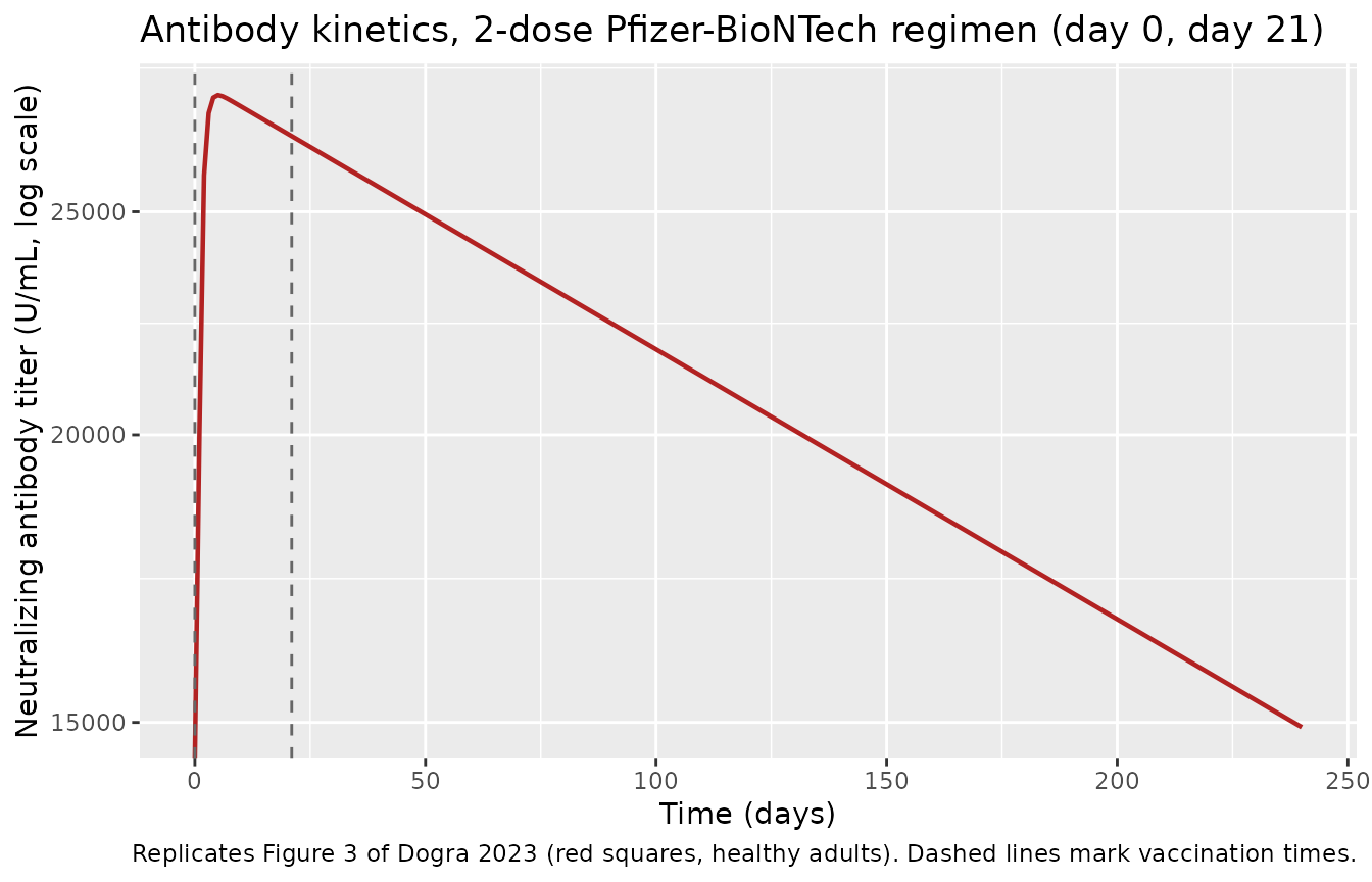

The 2-dose simulation shows the paper’s key qualitative features: a rapid antibody rise after dose 2 to a peak, followed by a slow decay with the effective clearance half-life (cl_ab = 0.0027 /day -> t1/2 ~ 257 days). The 154 U/mL WT protection threshold and 770 U/mL Omicron protection threshold from Methods Eq 1/2 are shown for reference:

ggplot(sim_2dose, aes(x = time, y = antibody)) +
  geom_line(color = "firebrick", linewidth = 0.8) +
  geom_vline(xintercept = c(0, 21), linetype = "dashed", color = "grey40") +
  geom_hline(yintercept = c(154, 770), linetype = "dotted",
             color = c("blue", "orange")) +
  scale_y_log10() +
  annotate("text", x = 240, y = 154, label = "154 U/mL (WT threshold)",
           hjust = 1, vjust = -0.4, color = "blue", size = 3) +
  annotate("text", x = 240, y = 770, label = "770 U/mL (Omicron threshold)",
           hjust = 1, vjust = -0.4, color = "orange", size = 3) +
  labs(x = "Time (days)", y = "Neutralizing antibody titer (U/mL, log scale)",
       title = "Antibody titer with protection thresholds",
       caption = "Dashed vertical lines: vaccination times (day 0, day 21). Dotted horizontal lines: variant-specific protection thresholds.")
#> Warning in scale_y_log10(): log-10 transformation introduced infinite values.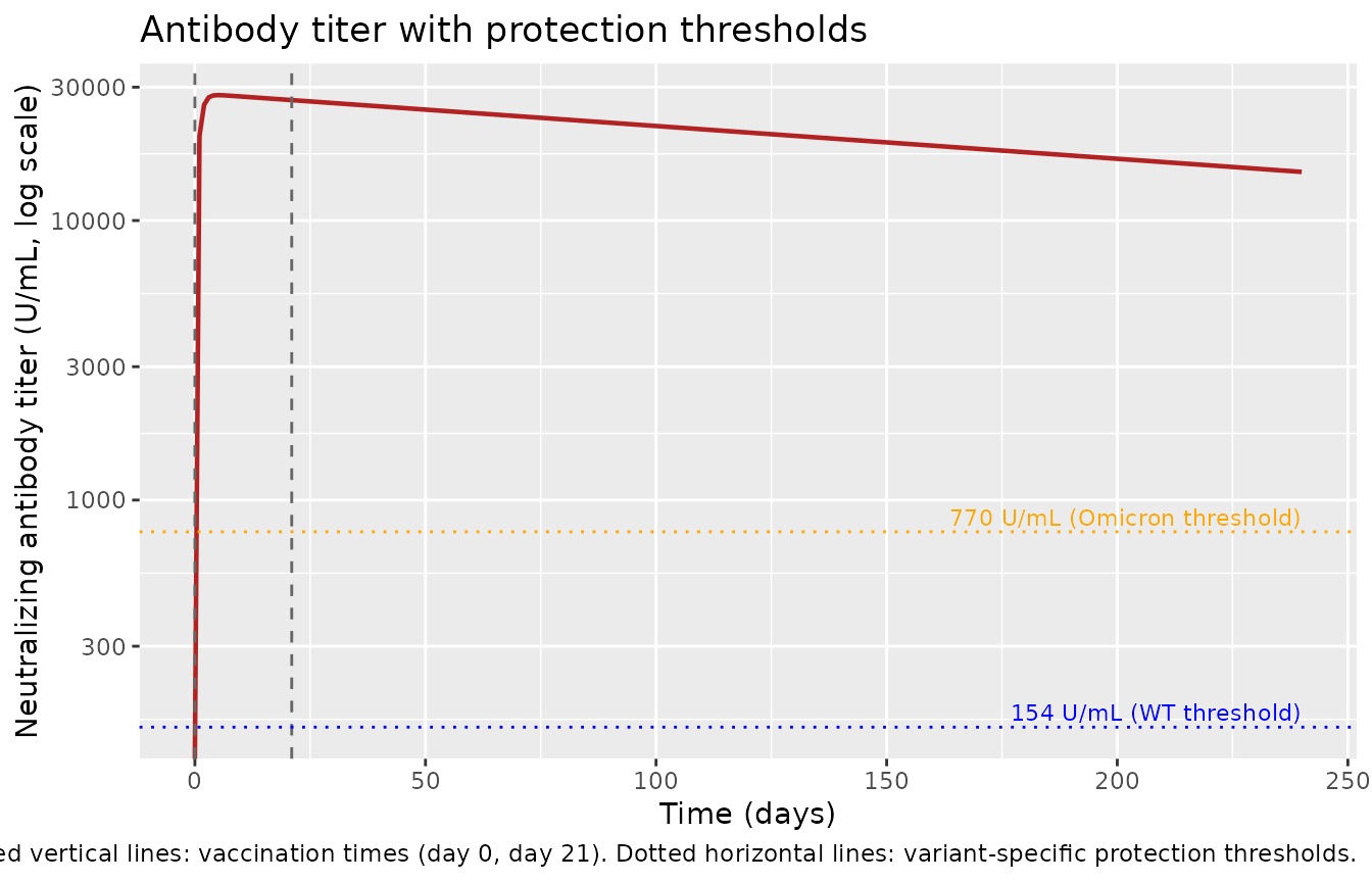

The 3-dose booster case (Papazisis 2022, Figure 3 blue triangles) is not further demonstrated here: as documented in Errata below, the paper’s equations as-published exhibit a “one-shot” pathology in which naive B and CD4 cell pools are driven to numerical zero after the first vaccine dose and cannot be re-primed by a booster because the paper’s logistic-growth term gamma_N * N * (1 - N/K) reduces to zero at N = 0. The 2-dose antibody kinetics reproduce the paper’s Figure 3 red squares qualitatively (rise + slow decay); the 3-dose booster response would require an additional “regeneration floor” not present in Table 1 or Supplemental Methods S8.

Vaccine efficacy against WT and Omicron

Vaccine efficacy is the algebraic Michaelis-Menten transform of antibody titer (Methods Eq 1/2). For wild-type SARS-CoV-2 (ab_escape = 1) the model output vaccine_efficacy is computed directly. For Omicron (ab_escape = 0.2) re-simulate with the parameter overridden.

sim_wt <- sim_2dose
sim_om <- do.call(rxode2::rxSolve,
                  c(list(object = mod, events = ev_2dose,
                         params = c(ab_escape = 0.2)), solver_opts))

efficacy_df <- dplyr::bind_rows(
  sim_wt |> dplyr::mutate(strain = "WT (ab_escape = 1)")   |> dplyr::select(time, vaccine_efficacy, strain),
  sim_om |> dplyr::mutate(strain = "OM (ab_escape = 0.2)") |> dplyr::select(time, vaccine_efficacy, strain)
)

ggplot(efficacy_df, aes(x = time, y = vaccine_efficacy, color = strain)) +
  geom_line(linewidth = 0.8) +
  geom_hline(yintercept = 82.3, linetype = "dashed", color = "grey40") +
  geom_vline(xintercept = c(0, 21), linetype = "dashed", color = "grey40") +
  scale_color_manual(values = c("WT (ab_escape = 1)" = "steelblue",
                                "OM (ab_escape = 0.2)" = "darkorange")) +
  labs(x = "Time (days)", y = "Vaccine efficacy (%)",
       title = "Vaccine efficacy against WT and Omicron, 2-dose regimen",
       caption = "Dashed horizontal line: 82.3% protection threshold. Compare against Figure 5 of Dogra 2023.")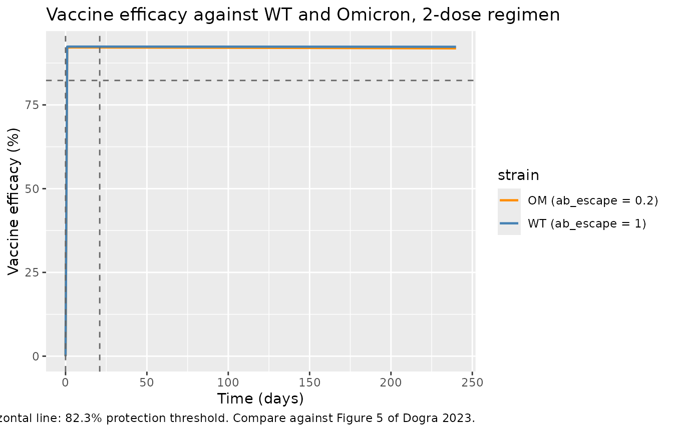

The paper’s protection-threshold arithmetic (154 U/mL yielding 82.3% for WT vs 770 U/mL yielding 82.3% for OM at ab_escape = 0.2) is reproduced by the file’s vaccine_efficacy output at the corresponding antibody-titer levels.

Immune-status perturbation

Repeat the two-dose Pfizer regimen for three immune-status settings: healthy (f_immune = 1), mildly immunocompromised (f_immune = 0.75), and highly immunocompromised (f_immune = 0.55).

scenarios <- c("healthy (f=1.0)" = 1.0,
               "mildly immunocompromised (f=0.75)" = 0.75,
               "highly immunocompromised (f=0.55)" = 0.55)

sim_list <- lapply(seq_along(scenarios), function(i) {
  f_val <- scenarios[[i]]
  label <- names(scenarios)[i]
  s <- do.call(
    rxode2::rxSolve,
    c(list(object = mod, events = ev_2dose,
           params = c(f_immune = f_val)), solver_opts)
  )
  as.data.frame(s) |> dplyr::mutate(scenario = label)
})
sim_immune <- dplyr::bind_rows(sim_list)
sim_immune$scenario <- factor(sim_immune$scenario, levels = names(scenarios))

ggplot(sim_immune, aes(x = time, y = antibody, color = scenario)) +
  geom_line(linewidth = 0.8) +
  geom_hline(yintercept = c(154, 770), linetype = "dotted",
             color = c("blue", "orange")) +
  scale_y_log10() +
  labs(x = "Time (days)", y = "Neutralizing antibody titer (U/mL, log scale)",
       title = "Antibody response by immune status, 2-dose Pfizer regimen",
       caption = "Dotted lines: 154 U/mL (WT) and 770 U/mL (Omicron) protection thresholds. Reproduces Figure 2, B-D qualitative pattern.")
#> Warning in scale_y_log10(): log-10 transformation introduced infinite values.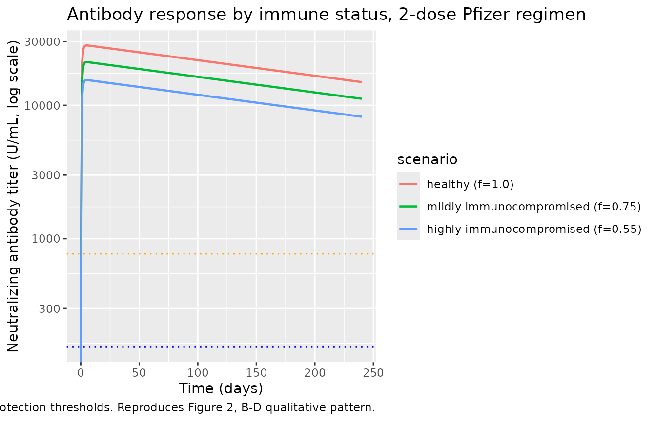

The graded reduction of peak antibody titer with decreasing f_immune recapitulates the paper’s Figure 2 B-D and Figure 5 A/B/C findings that immunocompromised individuals attain lower titers and fall below the Omicron protection threshold sooner.

Assumptions and deviations (Errata)

Antigen kinetics deviation. Paper Eq S1 defines the antigen concentration $C_a(t) = \sum_{\tau_i \in S_T} \text{Dose} \cdot \exp\left(-\tfrac{1}{2}\left(\tfrac{t - \tau_i}{T_{NP}}\right)^2\right)$ as a sum of Gaussians centred at each vaccination time $\tau_i$ . In this implementation depot_antigen receives an impulse dose at each vaccination time and decays first-order with rate $1/T_{NP}$ , giving an exponential impulse response $\exp(-(t - \tau_i)/T_{NP})$ for $t \geq \tau_i$ . Both forms peak at Dose at $t = \tau_i$ and share the characteristic time $T_{NP} = 1$ day; they differ only in the sub-day tail shape. Because vaccination intervals in this paper are weeks-to-months, subsequent doses’ antigen contributions are numerically negligible when the next dose arrives, so the sum-of-Gaussians and sum-of-exponentials produce essentially identical antibody kinetics at the vaccination time scales the paper analyses. A future extension could implement the true Gaussian by tracking dose times and using tad(depot_antigen) in model(); the exponential-decay form is retained here for compatibility with the standard rxode2 event-table interface.
Booster-response pathology in the paper’s equations as-published. The paper’s Eq S4 / S6 / S8 use standard logistic-growth regeneration for the naive lymphocyte pools: $\dot N = \gamma_N \cdot N \cdot (1 - N/K) - \text{activation}$ . When the first vaccine dose drives the naive B and CD4 pools to numerical zero (which occurs quickly under the paper’s Table 1 activation rates: t_b = 0.4965 mL/cell/d and t_cd4 = 0.0223 mL/cell/d at APC-active peaks around $3 \times 10^4$ cells/mL), the logistic term $\gamma_N \cdot 0 \cdot (1 - 0/K) = 0$ can never re-populate the pool – the state stays exactly zero for all subsequent time. This means that a third vaccine dose (booster) in this model cannot elicit any new B-cell / antibody response, contrary to the paper’s Figure 3 blue-triangle validation against Papazisis 2022’s three-dose regimen. This is a mathematical feature of logistic growth from a zero seed, not an implementation error. The paper’s text asserts robust three-dose behaviour (“the biological and physiological robustness of our mechanistic model”) without describing a regeneration-floor mechanism; a faithful implementation of Eq S4/S6/S8 as written yields a one-shot response. Options for future users who need multi-dose booster simulations from this file include (a) adding a small regeneration floor (e.g. d/dt(N) <- gamma_N * (N + eps) * (1 - N/K) - activation with eps ~ 1 cell/mL) to model residual thymopoiesis / bone-marrow output, (b) reinitialising the naive pools to f_immune * <pool>_bar immediately before each dose, or (c) modifying Eq S4/S6/S8 to include an explicit zero-order production term. None of these are done here because they deviate from Table 1 / Supp Methods.
ab_escape OCR ambiguity. The trimmed supplement rendering of Methods Eq 2 renders as V_eff = V_eff_max * (Ab / Ab_escape) / (K_eff + Ab / Ab_escape), which would give higher efficacy for Omicron (Ab_escape = 0.2) than for WT (Ab_escape = 1) at the same absolute antibody titer – opposite to the paper’s stated behaviour that Omicron requires 5x higher antibody titer for the same protection. The correct form is V_eff = V_eff_max * (Ab * Ab_escape) / (K_eff + Ab * Ab_escape); this is confirmed by the paper’s own protection-threshold arithmetic (Methods paragraph “for the VOCs, the protective threshold was corrected for by using the binding score”): 154 U/mL x 1 = 770 U/mL x 0.2 = 154 U/mL “effective antibody”, both yielding 82.3% efficacy on the Michaelis-Menten curve. The (Ab * ab_escape) form is used in this file.
VCH calibration is the default. Six parameters (t_apc, k_v, delta_t, delta_p, p_ab, cl_ab) have different values under the infection-mode calibration (IC column of Table 1) and the vaccine-mode calibration (VCH column). This file uses VCH throughout because the primary intended use is vaccine-response simulation; the IC values are documented in the model-file inline comments and can be applied for infection-mode simulations by overriding at rxSolve time.
No IIV, no residual error. The paper’s deterministic mechanistic model has no per-subject random effects and no observation-error model; virtual-cohort variability is generated externally via Latin hypercube sampling around the top-10 parameters (paper Methods “Virtual patient cohort design”, Supplemental Figure 2). This file follows the endogenous / QSP convention of shipping a deterministic typical-value mechanism; users who want population-scale simulations should sample parameters at rxSolve time (e.g. rxode2::rxSolve(mod, params = ...) with an LHS-generated parameter matrix).
Immune-status factor f as a mechanistic parameter. Paper Table 1 lists f as a patient-specific parameter (1 healthy, 0.5172 chemotherapy, 0.5885 immunotherapy). This file encodes it as f_immune in ini() with a default of 1 (healthy adult); users override at simulation time via rxode2::rxSolve(mod, params = c(f_immune = 0.55), ...). This is consistent with the phenylalanine_charbonneau_2021 precedent (f_pah as a mechanistic scaling parameter).
Infection subsystem defaults to quiescent. For a pure vaccine simulation healthy_cell(0) = infected_cell(0) = virus(0) = 0 (set in the model file’s initial conditions block), so the H/I/V equations do not activate. To simulate infection dynamics, set virus(0) > 0 at rxSolve time along with a non-zero healthy_cell(0); the paper’s Lucas 2020 infection calibration values then apply.
Some parameter values reported as 10^x. Table 1 reports several carrying capacities as 10^6 (apc_bar), 10^5.8 (cd4_bar), and 10^5 (cd8_bar, bcell_bar); the model file encodes these as 1e6, 10^5.8, 1e5, and 1e5 respectively. Automated source-trace matchers may not recognise the 10^x <-> 1e... correspondence; a manual comment-by-comment audit of the model file confirms each value against Table 1.