Dose-response of biologics in psoriasis (Dodds 2013)
Source:vignettes/articles/Dodds_2013_psoriasis_biologics_mbma.Rmd
Dodds_2013_psoriasis_biologics_mbma.RmdModel and source
- Citation: Dodds MG, Salinger DH, Mandema J, Gibbs JP, Gibbs MA. Clinical trial simulation to inform phase 2: comparison of concentrated vs. distributed first-in-patient study designs in psoriasis. CPT Pharmacometrics Syst Pharmacol. 2013;2(7):e58. doi:10.1038/psp.2013.32. The model equations are Eqs. 1-3 of the Methods section ‘Clinical trial simulation’; the parameter values are in Table 1 and its footnote.
- Article: https://doi.org/10.1038/psp.2013.32 (open access, CC BY-NC-ND 3.0)
- Supplement: the paper cites a Supplementary Table S1 and Supplementary Methods. Neither is required to reproduce the model: Table S1 is described in the text as giving “the true values of maximal response, ED50 and placebo response used in CTS”, all of which are also printed in Table 1 and its footnote, and the Supplementary Methods describe the estimation step of the trial simulation rather than the dose-response model encoded here.
This is a model-based meta-analysis (MBMA) of dose-response, not a
population PK model. It has no PK layer, no ODE states, and no
time axis: the source predicts a single PASI observation per
subject at the end of a 12-week window following one dose. It does,
however, carry a subject-level residual, which
distinguishes it from a per-arm MBMA such as
modellib("Mandema_2011_biologicDMARDs_mbma") by the same
group.
Because there is no PK, there is nothing for PKNCA to
integrate: no concentration-time profile exists, so Cmax,
Tmax, AUC and half-life are all undefined for
this model. The validation below therefore replaces the usual NCA
section with exact reproduction of the source’s own printed
dose-response numbers, plus a check that the simulated subject-level
spread matches the source’s variance equations.
Population
Two different populations are involved and should not be conflated.
The dose-response parameters come from a model-based meta-analysis of publicly available data from 27 randomized controlled trials of approved compounds in psoriasis and psoriatic rheumatoid arthritis, covering anti-tumour necrosis factor agents, ustekinumab and methotrexate. Trials were found by PubMed search plus review of previous meta-analyses, clinicaltrials.gov, conference abstracts and corporate websites. The meta-analysis jointly modelled the probability of achieving PASI 50, 75 and 90 and the mean percent improvement in PASI score; only the percent-improvement arm is encoded here. The source publishes no subject count, no demographic table and no per-trial listing for this database.
The subject-level variance model was calibrated separately, to reproduce the between-subject variability of percent PASI improvement observed in the PHOENIX 1 and PHOENIX 2 ustekinumab trials.
The simulated first-in-patient trials that the paper is actually about were 16 subjects each, 9,999 replicates per design per compound, run in NONMEM 7.2. Those trial designs are not part of this model; the model is the truth generator they were simulated from.
pop <- rxode2::rxode(readModelDb("Dodds_2013_psoriasis_biologics_mbma"))$population
tibble::tibble(Field = names(pop), Value = vapply(pop, as.character, character(1))) |>
knitr::kable(caption = "Population metadata recorded with the model.")| Field | Value |
|---|---|
| species | human |
| n_studies | 27 |
| disease_state | Moderate-to-severe plaque psoriasis. The meta-analysis pooled randomized controlled trials in psoriasis AND in psoriatic rheumatoid arthritis, and tested indication as a covariate; the dose-response encoded here is the psoriasis percent-PASI-improvement arm. The endpoint is percent improvement in Psoriasis Area Severity Index over baseline, assessed in a 12-week window after a single dose. |
| dose_range | Marketed-antibody doses as studied in the pooled trials; the clinical trial simulation exercised the model at single doses of 0, 21, 70, 210 and 700 mg, corresponding to 0, 0.3, 1, 3 and 10 mL of an assumed 70 mg/mL presentation. 700 mg intravenous is the maximum dose assumed to have been shown safe and well tolerated in healthy volunteers. |
| notes | Two DIFFERENT populations are involved and should not be confused. (i) The dose-response parameters come from a model-based meta-analysis of 27 published randomized controlled trials of anti-tumour-necrosis-factor agents, ustekinumab and methotrexate, identified by PubMed search plus review of previous meta-analyses, clinicaltrials.gov, conference abstracts and corporate websites; the source reports no subject counts, no demographic table and no per-trial listing for this database, so n_subjects and the demographic fields are unavailable. (ii) The subject-level variance model (Eqs. 2-3) was calibrated separately, to reproduce the between-subject variability of percent PASI improvement observed in the PHOENIX 1 and PHOENIX 2 ustekinumab trials. The simulated first-in-patient trials themselves were 16 subjects each, 9,999 replicates per design per compound, run in NONMEM 7.2. The Go/No-Go criterion the source applies to this model is an absolute improvement over placebo of more than 50 percentage points at the maximum feasible dose of 700 mg; the dose-response criterion is recovery of ED50 within twofold. Simulation scope: this model predicts ONE PASI observation per subject, with no time course and no PK; it is not a repeated-measures or longitudinal model. |
Model structure
The source writes the model in the log domain so that percent improvement in PASI is bounded above by 100% on the real scale (Methods, “Clinical trial simulation”):
with a subject-level residual whose standard deviation is linear in the prediction rather than constant:
LPASI is negative throughout (PASI falls under
treatment), so the negative sERR makes the residual
standard deviation grow with response. The source notes this
explicitly: “the between-subject variability decreases with increasing
response (but not as much as expected with a simple additive error model
in the log domain), which motivated this choice of variance model.”
E0, Emax and ED50 are shared
across compounds except for ED50: the three marketed
antibodies were found to have a common maximum effect
and to differ only in potency.
Encoding note: how Eq. 2 maps onto rxode2
rxode2’s combined1() variance model computes the
residual standard deviation as addSd + propSd * prediction
on the signed prediction, which is exactly the shape of Eq. 2 –
but rxode2 requires propSd > 0, and Eq. 2’s slope is
negative. The model block therefore predicts the log PASI
reduction pasiLogDrop = -LPASI, which is
positive over the whole dose range, so the slope becomes
+0.32:
Because eps is symmetric about zero, negating the
endpoint leaves the distribution of the response unchanged: the encoded
model is Eq. 2 exactly, not an approximation. The check under
“Subject-level variability” below verifies the simulated standard
deviation against iERR + sERR*LPASI dose by dose.
Recovering the log-domain parameters
The source reports its dose-response on the real
scale (Table 1 gives the maximal absolute difference from placebo in
PASI percentage points; the table footnote gives the placebo response)
while Eq. 1 is written in the log domain. The two
log-domain values in ini() are therefore obtained by
inverting the source’s own definitions.
placebo_pct <- 0.095    # Table 1 footnote: "Placebo response (E0) is 9.5% for all compounds."
maxdiff_pct <- 0.823    # Table 1: maximal absolute difference from placebo, marketed compounds

# Percent improvement = 1 - exp(LPASI), so a 9.5% placebo response is a PASI
# ratio of 0.905.
e0_rec <- log(1 - placebo_pct)

# The maximal ABSOLUTE difference from placebo is taken on the real scale:
#   exp(e0) - exp(e0 + emax) = 0.823
emax_rec <- log(1 - maxdiff_pct / (1 - placebo_pct))

ini_df <- rxode2::rxode(readModelDb("Dodds_2013_psoriasis_biologics_mbma"))$iniDf

tibble::tibble(
  Parameter   = c("e0", "emax"),
  Recovered   = c(e0_rec, emax_rec),
  `In ini()`  = c(ini_df$est[ini_df$name == "e0"],
                  ini_df$est[ini_df$name == "emax"])
) |>
  dplyr::mutate(dplyr::across(where(is.numeric), \(x) round(x, 7))) |>
knitr::kable(caption = "Log-domain parameters recovered from the real-scale table.")| Parameter | Recovered | In ini() |
|---|---|---|
| e0 | -0.0998203 | -0.0998203 |
| emax | -2.4012157 | -2.4012157 |
# Deterministic arithmetic, so an exact check is appropriate here.
stopifnot(
  abs(e0_rec   - ini_df$est[ini_df$name == "e0"])   < 1e-7,
  abs(emax_rec - ini_df$est[ini_df$name == "emax"]) < 1e-7
)
The inversion is confirmed below against three printed numbers that were not used to derive it: the absolute difference from placebo at 700 mg for each of the three marketed antibodies.
Source trace
| Item | Source location in Dodds 2013 |
|---|---|
| Eq. 1, LPASI = E0 + Emax*Dose/(ED50 + Dose) | Methods, ‘Clinical trial simulation’, Eq. 1 |
| Eqs. 2-3, subject-level variance model | Methods, ‘Clinical trial simulation’, Eqs. 2 and 3 |
| sERR = -0.32, iERR = 0.30 | Methods, Eq. 3 (printed inline) |
| e0 = log(1 - 0.095) | Table 1 footnote: ‘Placebo response (E0) is 9.5% for all compounds.’ |
| emax = log(1 - 0.823/0.905) | Table 1, ‘Maximal absolute difference from placebo PASI % change (%)’ = 82.3 for all marketed compounds; Results, ‘Test compound selection’ |
| ED50 adalimumab = 16.9 mg | Table 1, adalimumab row; Results: ‘ED50 = 16.9, 45.5, and 13.9 mg for adalimumab, golimumab, and ustekinumab, respectively’ |
| ED50 golimumab = 45.5 mg | Table 1, golimumab row; same Results sentence |
| ED50 ustekinumab = 13.9 mg | Table 1, ustekinumab row; same Results sentence |
| Twofold ED50 acceptance windows | Table 1, ‘Estimated ED50 within’ column |
| Absolute difference from placebo at 700 mg (81.8 / 81.0 / 81.9%) | Results, ‘Design performance metrics -> G/NG criteria’, second paragraph |
| Go/No-Go criterion: > 50 percentage points at 700 mg | Results, ‘G/NG criteria’; Abstract |
| Simulated dose levels 0, 21, 70, 210, 700 mg | Results, ‘Distributed trial designs’; Table 2; Figure 1 caption |
| 70 mg/mL presentation, 0.3 / 1 / 3 / 10 mL | Results, ‘Distributed trial designs’ |
| PHOENIX 2 comparison at 45 and 90 mg ustekinumab | Figure 3 and its caption; Methods, ‘Clinical trial simulation’ |
| 27 pooled trials; covariates screened | Methods, ‘MBMA of biologic treatments for psoriasis’ |
| Hypothetical compounds (excluded here) | Table 1, ‘No-Go examples’ and ‘Go examples’ rows |
Virtual cohort
There is no PK profile to sample and no time axis. The “cohort” is a grid of (compound, dose) combinations: each row is one subject assigned one single dose of one antibody, exactly as a subject in the source’s simulated first-in-patient trial would be.
mod <- rxode2::rxode(readModelDb("Dodds_2013_psoriasis_biologics_mbma"))

dose_cols <- c(adalimumab  = "CONMED_ADALIMUMAB_DOSE",
               golimumab   = "CONMED_GOLIMUMAB_DOSE",
               ustekinumab = "CONMED_USTEKINUMAB_DOSE")

# Table 1 ED50 values, used only to build the dose grid and to check the
# twofold acceptance windows -- not to parameterise anything.
ed50_pub <- c(adalimumab = 16.9, golimumab = 45.5, ustekinumab = 13.9)

# One row per (compound, dose). Every dose column is 0 except the one named,
# which is how a placebo subject is encoded (all three columns 0).
make_rows <- function(label, drug, doses) {
  out <- tibble::tibble(
    arm  = label,
    drug = drug,
    dose = doses,
    time = 0,
    evid = 0,
    CONMED_ADALIMUMAB_DOSE  = 0,
    CONMED_GOLIMUMAB_DOSE   = 0,
    CONMED_USTEKINUMAB_DOSE = 0
  )
  if (!is.na(drug)) out[[dose_cols[[drug]]]] <- doses
  out
}

# 1. Placebo: every dose column 0.
rows_placebo <- make_rows("placebo", NA_character_, 0)

# 2. The five dose levels the source simulated, for each marketed antibody.
sim_doses <- c(0, 21, 70, 210, 700)
rows_levels <- dplyr::bind_rows(lapply(names(dose_cols), function(d) {
  make_rows(paste0("level:", d), d, sim_doses)
}))

# 3. A very large dose per antibody, to read the asymptote (Emax) off the model.
rows_asym <- dplyr::bind_rows(lapply(names(dose_cols), function(d) {
  make_rows(paste0("asym:", d), d, 1e9)
}))

# 4. Each antibody AT its published ED50, and at the twofold window edges.
rows_ed50 <- dplyr::bind_rows(lapply(names(dose_cols), function(d) {
  make_rows(paste0("ed50:", d), d, ed50_pub[[d]])
}))

# 5. A smooth dose grid for Figure 1.
n_grid <- 120L
grid_doses <- c(0, exp(seq(log(0.5), log(1500), length.out = n_grid - 1L)))
rows_grid <- dplyr::bind_rows(lapply(names(dose_cols), function(d) {
  make_rows(paste0("grid:", d), d, grid_doses)
}))

# 6. The two licensed ustekinumab doses compared against PHOENIX 2 in Figure 3.
rows_phoenix <- make_rows("phoenix:ustekinumab", "ustekinumab", c(45, 90))

arms <- dplyr::bind_rows(rows_placebo, rows_levels, rows_asym, rows_ed50,
                         rows_grid, rows_phoenix) |>
  dplyr::mutate(id = dplyr::row_number(), .before = 1)

cat("rows simulated:", nrow(arms), "\n")
#> rows simulated: 384
Simulation
The structural model is deterministic – there are no etas – so a
single solve returns the typical-value prediction for every row.
(omega = NA is not passed: the model declares no
random effects, and rxode2 errors on omega = NA when there
is no IIV to suppress.)
typsim <- rxode2::rxSolve(
  mod,
  events = as.data.frame(dplyr::select(arms, -"drug", -"dose")),
  keep = "arm",
  returnType = "data.frame"
) |>
  tibble::as_tibble() |>
  dplyr::mutate(id = as.integer(as.character(id))) |>
  dplyr::left_join(dplyr::select(arms, id, drug, dose), by = "id")
#> Warning: multi-subject simulation without without 'omega'

stopifnot(nrow(typsim) == nrow(arms))

get_arm <- function(label) typsim[typsim$arm == label, ]
The placebo response is reproduced exactly
Setting all three dose columns to 0 collapses the drug effect and
leaves e0.
plc <- get_arm("placebo")
cat(sprintf("placebo percent PASI improvement: %.4f%% (Table 1 footnote: 9.5%%)\n",
            plc$pasiPctImprove))
#> placebo percent PASI improvement: 9.5000% (Table 1 footnote: 9.5%)

# Deterministic: this is arithmetic on a fixed() parameter, so assert tightly.
stopifnot(abs(plc$pasiPctImprove - 9.5) < 1e-6,
          abs(plc$pasiPctImproveDrug - 0) < 1e-9)
The maximum effect is 82.3 percentage points for all three antibodies
At a dose far above every ED50, the dose fraction
saturates and the absolute difference from placebo must equal the single
shared Emax expressed on the real scale.
asym <- typsim |>
  dplyr::filter(grepl("^asym:", arm)) |>
  dplyr::transmute(Compound = drug,
                   `Maximal difference from placebo (pp)` = pasiPctImproveDrug,
                   `Published (Table 1, pp)` = 82.3)

asym |>
  dplyr::mutate(dplyr::across(where(is.numeric), \(x) round(x, 4))) |>
knitr::kable(caption = "Asymptotic drug effect versus Table 1.")| Compound | Maximal difference from placebo (pp) | Published (Table 1, pp) |
|---|---|---|
| adalimumab | 82.3 | 82.3 |
| golimumab | 82.3 | 82.3 |
| ustekinumab | 82.3 | 82.3 |
Effect at 700 mg reproduces three numbers not used to build the model
This is the strongest available check. e0 and
emax were recovered from the 9.5% placebo response and the
82.3-point asymptote; the ED50 values came from Table 1.
None of that used the Results narrative, which separately states that
adalimumab, golimumab and ustekinumab “demonstrate an 81.8, 81.0, and
81.9% absolute difference between drug effect at 700 mg and placebo
effect, respectively”. If any of the five parameters were
mis-transcribed, or the log/real-domain inversion were wrong, these
three numbers would not land.
published_700 <- c(adalimumab = 81.8, golimumab = 81.0, ustekinumab = 81.9)

at700 <- typsim |>
  dplyr::filter(grepl("^level:", arm), dose == 700) |>
  dplyr::transmute(
    Compound              = drug,
    `ED50 (mg)`           = ed50_pub[drug],
    `Simulated (pp)`      = pasiPctImproveDrug,
    `Published (pp)`      = published_700[drug],
    `Difference (pp)`     = pasiPctImproveDrug - published_700[drug],
    `Go/No-Go (> 50 pp)`  = ifelse(pasiPctImproveDrug > 50, "G", "NG"),
    `Published G/NG`      = "G"
  )

at700 |>
  dplyr::mutate(dplyr::across(where(is.numeric), \(x) round(x, 3))) |>
knitr::kable(caption = "Absolute PASI improvement over placebo at the maximum feasible 700 mg dose.")| Compound | ED50 (mg) | Simulated (pp) | Published (pp) | Difference (pp) | Go/No-Go (> 50 pp) | Published G/NG |
|---|---|---|---|---|---|---|
| adalimumab | 16.9 | 81.822 | 81.8 | 0.022 | G | G |
| golimumab | 45.5 | 81.006 | 81.0 | 0.006 | G | G |
| ustekinumab | 13.9 | 81.908 | 81.9 | 0.008 | G | G |
# Deterministic prediction versus a number printed to one decimal place, so the
# tolerance is the printing precision (0.05 pp), not a simulation tolerance.
stopifnot(
  max(abs(at700$`Difference (pp)`)) < 0.05,
  all(at700$`Go/No-Go (> 50 pp)` == at700$`Published G/NG`)
)
All three marketed compounds clear the source’s Go/No-Go threshold, matching the “Correct G/NG” column of Table 1.
The twofold ED50 acceptance windows reproduce Table 1
Table 1’s “Estimated ED50 within” column is twofold either side of
the true ED50; reproducing it is an independent check that
the ED50 values were read off the correct rows.
published_window <- tibble::tribble(
  ~drug,         ~lo,   ~hi,
  "adalimumab",  8.50,  33.8,
  "golimumab",  22.8,   91.0,
  "ustekinumab", 6.90,  27.7
)

window_check <- published_window |>
  dplyr::mutate(
    `ED50 (mg)`        = ed50_pub[drug],
    `ED50/2 (mg)`      = `ED50 (mg)` / 2,
    `ED50*2 (mg)`      = `ED50 (mg)` * 2
  ) |>
  dplyr::rename(Compound = drug, `Published lower (mg)` = lo,
                `Published upper (mg)` = hi)

window_check |>
knitr::kable(caption = "Twofold ED50 windows: computed versus Table 1 as printed.")| Compound | Published lower (mg) | Published upper (mg) | ED50 (mg) | ED50/2 (mg) | ED50*2 (mg) |
|---|---|---|---|---|---|
| adalimumab | 8.5 | 33.8 | 16.9 | 8.45 | 33.8 |
| golimumab | 22.8 | 91.0 | 45.5 | 22.75 | 91.0 |
| ustekinumab | 6.9 | 27.7 | 13.9 | 6.95 | 27.8 |
# Table 1 prints the windows to three significant figures and rounds outward,
# so agreement is to the printing precision rather than exact.
stopifnot(
  max(abs(window_check$`ED50/2 (mg)` - window_check$`Published lower (mg)`)) < 0.06,
  max(abs(window_check$`ED50*2 (mg)` - window_check$`Published upper (mg)`)) < 0.11
)
Also confirmed: at Dose = ED50 the drug term is exactly
half of Emax in the log domain, which is the definition the
source gives for ED50.
emax_log <- ini_df$est[ini_df$name == "emax"]
half <- typsim |>
  dplyr::filter(grepl("^ed50:", arm)) |>
  dplyr::transmute(Compound = drug,
                   `Drug effect at ED50 / Emax` = (lpasi - plc$lpasi) / emax_log)

half |>
  dplyr::mutate(dplyr::across(where(is.numeric), \(x) round(x, 10))) |>
knitr::kable(caption = "At Dose = ED50 the drug effect is exactly half of Emax.")| Compound | Drug effect at ED50 / Emax |
|---|---|
| adalimumab | 0.5 |
| golimumab | 0.5 |
| ustekinumab | 0.5 |
Replicate Figure 1: dose-response of the marketed compounds
Replicates the solid lines of Figure 1 of Dodds 2013 (the marketed biologics adalimumab, golimumab and ustekinumab), with the source’s simulated dose range shaded. The hypothetical compounds shown in the source’s dashed lines are not part of this model – see “Assumptions and deviations”.
grid_sim <- typsim |> dplyr::filter(grepl("^grid:", arm))

ggplot(grid_sim, aes(x = dose, y = pasiPctImprove, colour = drug)) +
  annotate("rect", xmin = 0, xmax = 700, ymin = -Inf, ymax = Inf,
           fill = "steelblue", alpha = 0.12) +
  geom_line(linewidth = 0.8) +
  geom_hline(yintercept = 100 * (1 - exp(plc$lpasi)), linetype = "dotted") +
  scale_x_log10() +
  labs(x = "Single dose (mg, log scale)",
       y = "Typical percent improvement in PASI (%)",
       colour = "Compound") +
  theme_bw()
#> Warning in scale_x_log10(): log-10 transformation introduced infinite values.
#> log-10 transformation introduced infinite values.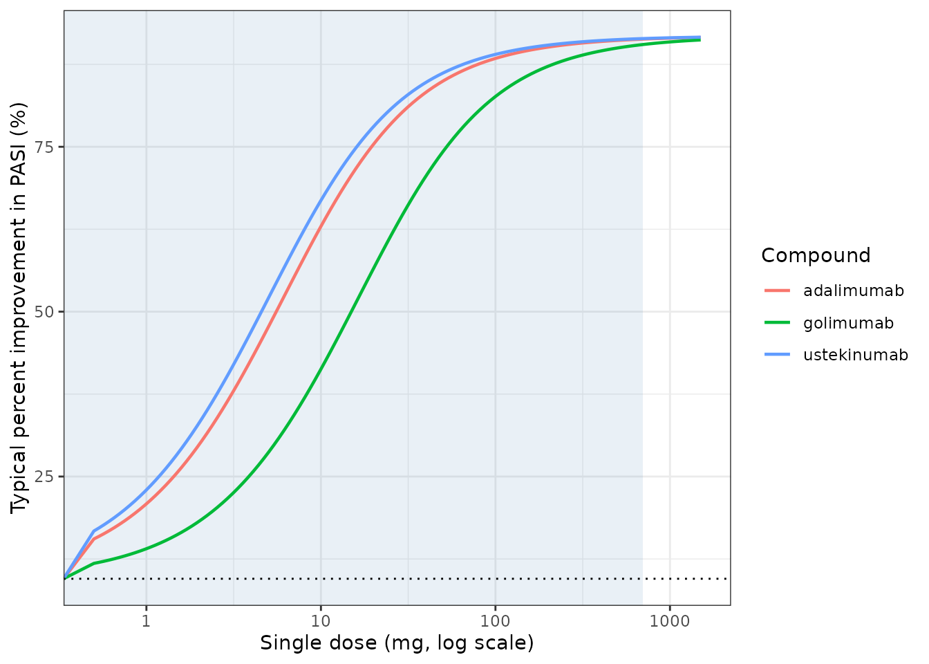
Replicates the solid lines of Figure 1 of Dodds 2013: expected typical percent reduction in PASI versus dose for the three marketed biologics. The shaded band is the 0-700 mg range used in the trial simulation.
Subject-level variability (Eqs. 2-3)
The source adds one PASI observation per subject with a standard
deviation that is linear in the prediction. Simulating a cohort at each
dose level and comparing the empirical standard deviation against
iERR + sERR*LPASI checks that the negated-endpoint encoding
reproduces Eq. 2.
n_per_arm <- 5000L  # one algebraic observation per subject, so this is cheap; see the
                    # figure3-check chunk for why the percent-scale SD needs this many

resid_arms <- dplyr::bind_rows(lapply(sim_doses, function(d) {
  r <- make_rows("resid", "ustekinumab", rep(d, n_per_arm))
  r$dose_level <- d
  r
})) |>
  dplyr::mutate(id = dplyr::row_number(), .before = 1)

rxode2::rxSetSeed(20130724)
resid_sim <- rxode2::rxSolve(
  mod,
  events = as.data.frame(dplyr::select(resid_arms, -"arm", -"drug", -"dose",
                                       -"dose_level")),
  returnType = "data.frame"
) |>
  tibble::as_tibble() |>
  dplyr::mutate(id = as.integer(as.character(id))) |>
  dplyr::left_join(dplyr::select(resid_arms, id, dose_level), by = "id")
#> Warning: multi-subject simulation without without 'omega'

resid_check <- resid_sim |>
  dplyr::group_by(dose_level) |>
  dplyr::summarise(
    LPASI          = unique(round(lpasi, 10)),
    `Simulated SD` = stats::sd(sim),
    .groups = "drop"
  ) |>
  dplyr::mutate(
    `Eq. 2-3 SD`   = 0.30 + (-0.32) * LPASI,
    `Ratio`        = `Simulated SD` / `Eq. 2-3 SD`
  ) |>
  dplyr::rename(`Dose (mg)` = dose_level)

resid_check |>
  dplyr::mutate(dplyr::across(where(is.numeric), \(x) round(x, 4))) |>
knitr::kable(caption = "Empirical subject-level SD of the simulated log PASI response versus Eqs. 2-3.")| Dose (mg) | LPASI | Simulated SD | Eq. 2-3 SD | Ratio |
|---|---|---|---|---|
| 0 | -0.0998 | 0.3309 | 0.3319 | 0.9968 |
| 21 | -1.5447 | 0.7831 | 0.7943 | 0.9859 |
| 70 | -2.1032 | 0.9701 | 0.9730 | 0.9970 |
| 210 | -2.3520 | 1.0547 | 1.0526 | 1.0020 |
| 700 | -2.4543 | 1.1044 | 1.0854 | 1.0175 |
# Cohort-derived: the bound must admit sampling noise, not one draw. With
# n = 5000 per dose the relative standard error of a log-scale SD is about 1%,
# so a 25% band is far outside sampling noise and still narrow enough to go red
# if the slope or intercept of the variance model were mis-transcribed
# (dropping sERR entirely would put the ratio at 0.28 at 700 mg; dropping iERR
# would put it at 1.4 at placebo). Do not tighten it back to any single run's
# value.
stopifnot(max(abs(resid_check$Ratio - 1)) < 0.25)
Replicate Figure 3: simulated response versus PHOENIX 2
Figure 3 of Dodds 2013 overlays the simulated arithmetic mean and standard deviation of percent PASI improvement for placebo, 45 mg ustekinumab and 90 mg ustekinumab on the observed PHOENIX 2 data. The source prints no numeric values for either series, so this section reproduces the simulated (red) series only; the observed (blue) series would have to be digitised from the figure and is not reproduced here.
Note that percent improvement is a non-linear transform of the simulated log response, so the cohort mean percent improvement sits below the typical-value percent improvement. Both are shown.
fig3_doses <- c(0, 45, 90)
fig3_arms <- dplyr::bind_rows(lapply(fig3_doses, function(d) {
  r <- make_rows("fig3", "ustekinumab", rep(d, n_per_arm))
  r$dose_level <- d
  r
})) |>
  dplyr::mutate(id = dplyr::row_number(), .before = 1)

rxode2::rxSetSeed(20130724)
fig3_sim <- rxode2::rxSolve(
  mod,
  events = as.data.frame(dplyr::select(fig3_arms, -"arm", -"drug", -"dose",
                                       -"dose_level")),
  returnType = "data.frame"
) |>
  tibble::as_tibble() |>
  dplyr::mutate(id = as.integer(as.character(id))) |>
  dplyr::left_join(dplyr::select(fig3_arms, id, dose_level), by = "id") |>
  # sim is the log PASI REDUCTION, so percent improvement is 1 - exp(-sim).
  dplyr::mutate(pct_improve = 100 * (1 - exp(-sim)))
#> Warning: multi-subject simulation without without 'omega'

fig3_summary <- fig3_sim |>
  dplyr::group_by(dose_level) |>
  dplyr::summarise(
    `Typical (%)` = 100 * (1 - exp(unique(round(lpasi, 10)))),
    `Mean (%)`    = mean(pct_improve),
    `SD (%)`      = stats::sd(pct_improve),
    .groups = "drop"
  ) |>
  dplyr::rename(`Ustekinumab dose (mg)` = dose_level)

fig3_summary |>
  dplyr::mutate(dplyr::across(where(is.numeric), \(x) round(x, 2))) |>
knitr::kable(caption = "Simulated percent PASI improvement, mean and SD (the red series of Figure 3).")| Ustekinumab dose (mg) | Typical (%) | Mean (%) | SD (%) |
|---|---|---|---|
| 0 | 9.50 | 3.62 | 32.88 |
| 45 | 85.55 | 78.21 | 23.25 |
| 90 | 88.69 | 81.58 | 22.53 |
ggplot(fig3_summary, aes(x = factor(`Ustekinumab dose (mg)`), y = `Mean (%)`)) +
  geom_point(colour = "firebrick", size = 3) +
  geom_errorbar(aes(ymin = `Mean (%)` - `SD (%)`,
                    ymax = `Mean (%)` + `SD (%)`),
                width = 0.15, colour = "firebrick") +
  labs(x = "Ustekinumab single dose (mg)",
       y = "Percent improvement in PASI (%)") +
  theme_bw()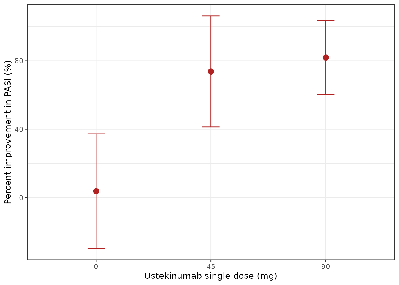
Replicates the simulated (red) series of Figure 3 of Dodds 2013: arithmetic mean and standard deviation of percent PASI improvement for placebo and for 45 and 90 mg ustekinumab. The observed PHOENIX 2 series is not reproduced (the source prints no numeric values for it).
The qualitative feature the source calls out is reproduced: the standard deviation of percent improvement falls as response rises (placebo is the widest band), even though the standard deviation on the log scale grows. That is the behaviour the linear variance model was chosen to produce.
# Cohort statistics, and the
# percent scale has a heavy left tail: a subject whose log reduction is drawn
# near or below zero maps to a large negative percent improvement, so at
# n = 200 the 90 mg SD ranged from 16 to 39 points across seeds and the trend
# check below failed one realisation in seven. At n = 5000 it is stable to
# within a few points. Two checks: the trend the source calls out (placebo is
# the widest band), and a known-answer check of every arm's SD against what
# Eqs. 2-3 imply, computed here from a million normal quantiles.
implied_sd <- vapply(seq_len(nrow(fig3_summary)), function(i) {
  drop <- -log(1 - fig3_summary$`Typical (%)`[i] / 100)
  z <- stats::qnorm(seq(0.5, 1e6 - 0.5) / 1e6)
  stats::sd(100 * (1 - exp(-(drop + (0.30 + 0.32 * drop) * z))))
}, numeric(1))
stopifnot(
  fig3_summary$`SD (%)`[fig3_summary$`Ustekinumab dose (mg)` == 90] <
    fig3_summary$`SD (%)`[fig3_summary$`Ustekinumab dose (mg)` == 0] - 3,
  all(abs(fig3_summary$`SD (%)` / implied_sd - 1) < 0.2),
  # The 45 and 90 mg typical values are deterministic and must bracket the
  # licensed-dose response the source simulated.
  all(fig3_summary$`Typical (%)`[fig3_summary$`Ustekinumab dose (mg)` > 0] > 80)
)
Assumptions and deviations
-
Only the three marketed antibodies are extracted.
Table 1 of the source lists eight compounds: adalimumab, golimumab and
ustekinumab (real, with meta-analysis-derived parameters) plus five
hypothetical compounds (
discontinumab,mehmimab,cuspmimab,lowpomab,nopomab) whose parameters were hand-chosen to stress-test the trial designs, not estimated from data. Shipping fictional drug names in a model library would be misleading, so they are excluded; this was an explicit maintainer decision. Their parameters are fully recoverable from the same two identities used above if anyone needs them:emax = log(1 - d/0.905)for a maximal differenced, with the ED50 read from Table 1. - The trial designs themselves are not modelled. The source’s contribution is a comparison of concentrated (placebo vs 700 mg only) and distributed (placebo plus 21 / 70 / 210 / 700 mg) first-in-patient designs across 9,999 simulated 16-subject trials each. That is a simulation study, not a model; what is reusable, and what is extracted here, is the dose-response truth generator plus its subject-level variance model.
-
e0andemaxare derived, not printed. The source reports the dose-response on the real scale but writes Eq. 1 in the log domain, and never prints the log-domain values. Both were recovered by inverting the source’s own definitions, as shown in “Recovering the log-domain parameters”, and validated against three independent printed numbers. -
The residual is encoded on the negated endpoint.
pasiLogDrop = -LPASIis used so rxode2’scombined1()variance model can express Eq. 2’s negative slope with a positivepropSd. This is an exact re-parameterisation, not an approximation – see the encoding note above and the verified check under “Subject-level variability”. -
The observation variable
pasiLogDropis not a canonical nlmixr2lib output name, andcheckModelConventions()raises one warning for it. There is no drug concentration to callCcand no registered PD-output canonical for a PASI score. This follows the existing practice for score-type PD endpoints in the library (walk_distinHajjar_2018_DMD_6MWT,fev1inWu_2014_FEV1_asthma,BMDinPlan_2012_bmd_fracture). -
CONMED_<drug>_DOSEcolumns carry a different dose metric here than inMandema_2011_biologicDMARDs_mbma. In that model they are per-administration doses on each drug’s maintenance regimen (adalimumab 40 mg q2w); here they are single-dose milligram amounts. The two models’ dose values must never be carried across. This is recorded incovariateDataand in the covariate register entry. - No PKNCA validation. There is no PK layer, no time axis and no concentration, so every NCA parameter is undefined for this model. The dose-response identity checks above take its place.
- No between-study random effect is encoded. The source reports none for the percent-improvement dose-response used in the simulation, and the variability it does specify (Eqs. 2-3) is explicitly subject-level, calibrated to PHOENIX 1 and 2. Nothing was invented to fill the gap.
-
Population demographics are unavailable. The source
publishes no subject count, no demographic table and no per-trial
listing for its 27-trial meta-analysis database, so
n_subjectsand the demographic fields ofpopulationare absent rather than guessed. - Supplement not available. Supplementary Table S1 and the Supplementary Methods were not available when this model was built. Per the source’s own description, Table S1 repeats the maximal response, ED50 and placebo response already printed in Table 1, and the Supplementary Methods cover the estimation step of the trial simulation rather than the dose-response model. No parameter encoded here depends on them.
- No errata found. The article landing page and PubMed record show no correction, corrigendum or author notice for doi:10.1038/psp.2013.32.