Lorlatinib signaling / shell-and-core tumor QSP (Braniff 2025)
Source:vignettes/articles/Braniff_2025_lorlatinib_qsp.Rmd
Braniff_2025_lorlatinib_qsp.RmdModel and source
- Citation: Braniff N, Joshi T, Cassidy T, Trogdon M, Kumar R, Poels K, Allen R, Musante CJ, Shtylla B. (2025). An integrated quantitative systems pharmacology virtual population approach for calibration with oncology efficacy endpoints. CPT Pharmacometrics Syst Pharmacol 14(2):268-278. doi:10.1002/psp4.13270
- Article: CPT Pharmacometrics Syst Pharmacol 14(2):268-278
Braniff et al. present a virtual-population (Vpop) selection algorithm for oncology quantitative systems pharmacology models that jointly matches tumor burden dynamics and progression-free survival in the presence of censoring. The mechanistic engine they use to demonstrate the algorithm - and the object extracted here - is a minimal MAPK/PI3K signaling model coupled to a shell-and-core tumor growth model, driven by the median plasma concentration time course of the ALK inhibitor lorlatinib. It was calibrated against a phase 2 non-small-cell lung cancer study.
Read this first. Braniff 2025 reports Vpop
sampling ranges, not point estimates, for the eleven quantities
its algorithm samples. The ini() values in the model file
are a single documented reference plausible patient; the published
ranges are what this vignette validates against. See Assumptions and deviations.
Population
The virtual populations were calibrated to the phase 2 lorlatinib study of Solomon et al. 2018 (NCT01970865) in adults with ALK-positive advanced NSCLC, dosed at lorlatinib 100 mg orally once daily. Braniff 2025 restricts the analysis to patients with at least two sum-of-longest-diameter (SLD) measurements and truncates follow-up at day 500, right-censoring everyone still on trial at that point. Virtual populations in Figures 4 and 5 are sized at 155 virtual patients to match the observed cohort.
Three endpoints are scored by the selection algorithm: baseline SLD (log-transformed before the scoring distribution is fit), best percentage change in SLD from baseline, and dropout time (time to progression or censoring, whichever came first). A two-component Gaussian mixture fit jointly to those three endpoints supplies the acceptance score.
Because the analysis fixes all PK covariates at their median values,
the model carries no inter-individual variability on
the PK parameters. Braniff 2025 Discussion states this explicitly: “in
this work we do not incorporate pharmacokinetic variability, instead
using a median model.” All population heterogeneity is generated by
sampling the eleven Vpop quantities plus the necrotic initial-condition
split phi_n0.
mod <- readModelDb("Braniff_2025_lorlatinib_qsp")()
ui  <- rxode2::rxode(mod)
Source trace
Every model equation and every ini() parameter, with its
location in the source. “Supplement” refers to the Supporting
Information of Braniff 2025 (PSP4-14-268-s001.docx,
published with the open-access article, PMC11812934).
| Component | Source |
|---|---|
| 2-compartment PK with sequential zero-/first-order absorption | Supplement S1, first equation block (attributed there to Chen 2021) |
| Time-varying clearance CL(t) = CLmax * (1 - exp(-kc * t)) | Supplement S1, ‘Time-dependent Clearance’ |
| pALK, RAS, pERK, pAKT, pS6 signaling relaxation equations | Supplement S1, second equation block |
| f_prolif, f_apop, k_kill drug-effect equations | Supplement S1, three displayed equations after the signaling block |
| Shell-and-core tumor ODEs (Np, Nn0..Nn4) | Supplement S1, third equation block; schematic in Figure 1 |
| Shell-to-core transfer rate kn | Supplement S1, displayed equation after the tumor block (see Assumptions) |
| Necrotic transit rate 1 / tau | Figure 1 schematic (Nn1 -> … -> Nn4 -> 0 arrows labelled 1/tau) |
| Np from delta_shell and rho_core; Nn_tot = rho_core * Np | Supplement S2, ‘Initial condition randomization (a)’ |
| Elimination rate ke from the bifurcation offset eps = 0.015 | Supplement S2, ‘Elimination rate computation (b)’ |
| phi_n0 randomisation bounds, Nn4 < kg0 * tau * Np | Supplement S2, ‘Initial condition randomization (a)’ |
| SLD = diameter of the combined shell-and-core mass | Figure 1 caption |
| 1e5 cells per microlitre (cell volume) | Supplement S1, sentence following the tumor ODE block |
| Parameter | Value | Source |
|---|---|---|
| lka | 74.712 1/day | Table S2 |
| lcl_exp_inf | 347.33 L/day | Table S2 (CLmax) |
| lcl_exp_kdes | 0.48 1/day | Table S2 (kc) |
| lvc | 120.51 L | Table S2 |
| lvp | 154.91 L | Table S2 |
| lq | 528.05 L/day | Table S2 |
| lfdepot | 0.759 | Table S2 (F) |
| ld1 | 0.047833 day | NOT in Braniff; Chen 2021 Table 4 D1 = 1.148 h, via Chen_2021_lorlatinib.R |
| lkout | 115.2 1/day | Table S2 (cited there to Yamazaki 2014) |
| imax | 1.0 | Table S2 (fitted to preclinical data) |
| lkkill_scale | 0.135 | Table S2 (theta_kkill, fitted to preclinical data) |
| lgfr_act | range 0.018-20 | Table S1; ini() value digitised from Figure 6a |
| lic50_drug | range 1.5-32.24 nM | Table S1; ini() value digitised from Figure S2 |
| lhill_drug | range 0.70-0.76 | Table S1; ini() value digitised from Figure S2 |
| lhill_prolif | range 0.28-5.02 (alpha) | Table S1; ini() value digitised from Figure 6a |
| lkc50_prolif | range 0.00025-36.56 | Table S1; ini() value digitised from Figure S2 |
| lhill_apop | range 0.21-6.24 (beta) | Table S1; ini() value digitised from Figure S2 |
| lkc50_apop | range 0.023-33.37 | Table S1; ini() value digitised from Figure S2 |
| lkg0 | range 0.1-1.5 1/day | Table S1; ini() value digitised from Figure 6a |
| ltau_necrotic | range 0.04-0.9 day | Table S1; ini() value digitised from Figure S2 |
| lrho_core | range 0.15-0.75 | Table S3; ini() value digitised from Figure S2 |
| ldelta_shell | range 0.07-1.3 cm | Table S3; ini() value digitised from Figure 6a |
| phi_n0 | U[phi_n0_min, 1] | Supplement S2; ini() value is the mean of that distribution |
| eps_bifurc | 0.015 | Supplement S2 |
| cell_vol | 1e-5 mm^3 | Supplement S1 (1e5 cells per microlitre) |
| mw_drug | 406.41 g/mol | Physical constant for lorlatinib; NOT a Braniff parameter |
| propSd, addSd_sld | fixed(0) | Braniff 2025 fits no residual-error model |
The published Vpop sampling ranges
vpop_ranges <- tibble::tribble(
  ~parameter,      ~lo,     ~hi,   ~source,
  "gfr_act",       0.018,   20,    "Table S1",
  "ic50_drug",     1.5,     32.24, "Table S1",
  "hill_drug",     0.70,    0.76,  "Table S1",
  "hill_prolif",   0.28,    5.02,  "Table S1",
  "kc50_prolif",   0.00025, 36.56, "Table S1",
  "hill_apop",     0.21,    6.24,  "Table S1",
  "kc50_apop",     0.023,   33.37, "Table S1",
  "kg0",           0.1,     1.5,   "Table S1",
  "tau_necrotic",  0.04,    0.9,   "Table S1",
  "rho_core",      0.15,    0.75,  "Table S3",
  "delta_shell",   0.7,     13,    "Table S3 (0.07-1.3 cm, expressed in mm)"
)
knitr::kable(vpop_ranges, caption = "Vpop sampling ranges (Braniff 2025 Tables S1 and S3).")| parameter | lo | hi | source |
|---|---|---|---|
| gfr_act | 0.01800 | 20.00 | Table S1 |
| ic50_drug | 1.50000 | 32.24 | Table S1 |
| hill_drug | 0.70000 | 0.76 | Table S1 |
| hill_prolif | 0.28000 | 5.02 | Table S1 |
| kc50_prolif | 0.00025 | 36.56 | Table S1 |
| hill_apop | 0.21000 | 6.24 | Table S1 |
| kc50_apop | 0.02300 | 33.37 | Table S1 |
| kg0 | 0.10000 | 1.50 | Table S1 |
| tau_necrotic | 0.04000 | 0.90 | Table S1 |
| rho_core | 0.15000 | 0.75 | Table S3 |
| delta_shell | 0.70000 | 13.00 | Table S3 (0.07-1.3 cm, expressed in mm) |
Event-table helper
The model defines two endpoints (Cc, plasma lorlatinib
in ng/mL; sld, the sum of longest diameters in mm), both of
which are algebraic rather than ODE states. Observation rows therefore
carry dvid and a missing cmt; doses go to the
depot compartment by name.
make_events <- function(obs_times, ids = 1L, dvid = 1L,
                        dose = 100, ii = 1, until = 500) {
  obs <- expand.grid(id = ids, time = obs_times)
  obs$evid <- 0L
  obs$amt  <- NA_real_
  obs$cmt  <- NA_character_
  obs$dvid <- as.integer(dvid)
  if (dose > 0) {
    dos <- expand.grid(id = ids, time = seq(0, until, by = ii))
    dos$evid <- 1L
    dos$amt  <- dose
    dos$cmt  <- "depot"
    dos$dvid <- NA_integer_
    obs <- rbind(dos, obs)
  }
  obs[order(obs$id, obs$time, -obs$evid), ]
}
Reference plausible patient
Signaling and tumor time course
ev_ref  <- make_events(seq(0, 500, by = 0.25))
sim_ref <- rxode2::rxSolve(ui, ev_ref, atol = 1e-8, rtol = 1e-8,
                           maxsteps = 1e5) |>
  as.data.frame() |>
  dplyr::filter(!is.na(sld))

sld0_ref <- sim_ref$sld[1]
sim_ref  <- dplyr::mutate(sim_ref, pct_change = 100 * (sld - sld0_ref) / sld0_ref)
sprintf("Reference-patient baseline SLD = %.2f mm", sld0_ref)
#> [1] "Reference-patient baseline SLD = 25.77 mm"
sim_ref |>
  dplyr::filter(time <= 14) |>
  dplyr::select(time, palk, ras, perk, pakt, ps6) |>
  tidyr::pivot_longer(-time, names_to = "species", values_to = "value") |>
  ggplot(aes(time, value, colour = species)) +
  geom_line(linewidth = 0.7) +
  labs(x = "Time (days)", y = "Fraction of untreated baseline", colour = NULL) +
  theme_bw()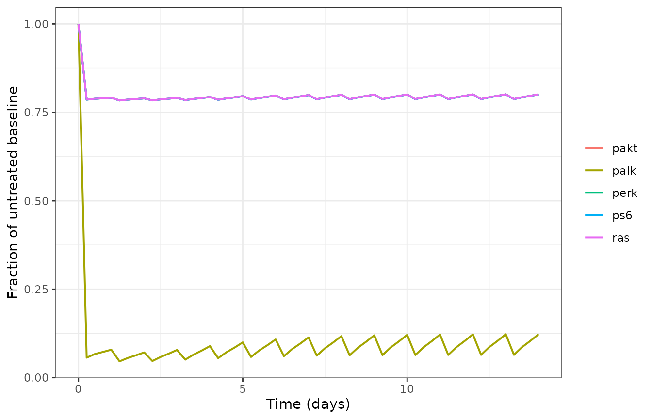
Normalised signaling species for the reference plausible patient on lorlatinib 100 mg once daily. Each species is 1 at the untreated baseline. Reproduces the pathway structure of Braniff 2025 Figure 1.
ggplot(sim_ref, aes(time / 7, pct_change)) +
  geom_hline(yintercept = c(20, -30), linetype = "dashed", colour = "grey40") +
  geom_line(linewidth = 0.7, colour = "firebrick") +
  labs(x = "Time (weeks)", y = "Change in SLD from baseline (%)") +
  theme_bw()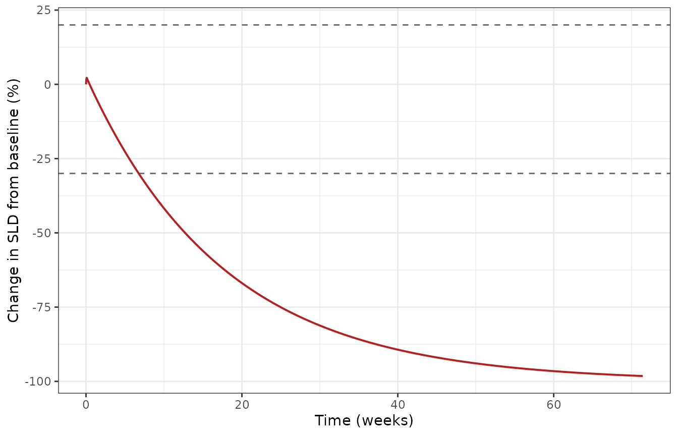
Reference-patient SLD trajectory on lorlatinib 100 mg once daily, with the RECIST progression (+20%) and partial-response (-30%) thresholds of Braniff 2025 Figure 4b.
Untreated-growth gate (Table S3)
Braniff 2025 rejects any candidate plausible patient whose untreated doubling time, measured over a six-week simulation “up to first scan”, falls outside 26-165 days (Table S3). This is a published constraint on the model, so the reference patient must satisfy it.
ev_untreated  <- make_events(seq(0, 42, by = 0.25), dose = 0)
sim_untreated <- rxode2::rxSolve(ui, ev_untreated, atol = 1e-8, rtol = 1e-8,
                                 maxsteps = 1e5) |>
  as.data.frame() |>
  dplyr::filter(!is.na(sld))

# SLD is a diameter, so the cell-count ratio is the cubed SLD ratio.
volume_ratio  <- (sim_untreated$sld[nrow(sim_untreated)] / sim_untreated$sld[1])^3
doubling_time <- 42 * log(2) / log(volume_ratio)

knitr::kable(
  tibble::tibble(
    Quantity  = "Untreated doubling time up to first scan",
    Simulated = sprintf("%.1f days", doubling_time),
    Required  = "26 - 165 days",
    Pass      = doubling_time >= 26 && doubling_time <= 165
  ),
  caption = "Braniff 2025 Table S3 untreated-growth constraint."
)| Quantity | Simulated | Required | Pass |
|---|---|---|---|
| Untreated doubling time up to first scan | 52.6 days | 26 - 165 days | TRUE |
Discriminating the two readings of the shell-to-core transfer rate
Braniff 2025 states that the tumor model “assumes the core-shell ratio remains constant”, and prints
Read with rho_core as the core-shell
ratio (sum(Nni) / Np), that expression
does not in fact hold the ratio constant. Read with
rho_core as the necrotic fraction
phi_n = rho_core / (1 + rho_core) - a quantity the
supplement defines and uses throughout Section S2 - it becomes
algebraically identical to the rate that does hold the ratio constant,
because 1 - phi_n = 1 / (1 + rho_core).
The paper’s own constraints settle which reading was intended. The ratio reading cannot reach the Table S3 untreated-growth window anywhere in the Table S1/S3 parameter space, and produces essentially static tumors; the fraction reading satisfies Table S3 and reproduces the Figure 4b shrinkage.
kn_ratio_reading <- rxode2::rxode({
  ktr   <- 1 / tau_necrotic
  grow  <- kg0 * cycling_cells
  clear <- ktr * damaged_cells5
  kn    <- (clear + rho_core * (grow - clear)) / cycling_cells
  d/dt(cycling_cells)  <- kg0 * cycling_cells - kn * cycling_cells
  d/dt(damaged_cells1) <- kn * cycling_cells - ke_necrotic * damaged_cells1
  d/dt(damaged_cells2) <- ke_necrotic * damaged_cells1 - ktr * damaged_cells2
  d/dt(damaged_cells3) <- ktr * (damaged_cells2 - damaged_cells3)
  d/dt(damaged_cells4) <- ktr * (damaged_cells3 - damaged_cells4)
  d/dt(damaged_cells5) <- ktr * (damaged_cells4 - damaged_cells5)
  n_tot <- cycling_cells + damaged_cells1 + damaged_cells2 +
           damaged_cells3 + damaged_cells4 + damaged_cells5
})

# Sweep the published bounds and record the fastest untreated doubling time
# the ratio reading can attain.
grid <- expand.grid(kg0 = c(0.1, 0.5, 1.0, 1.5),
                    tau_necrotic = c(0.04, 0.3, 0.6, 0.9),
                    rho_core = c(0.15, 0.35, 0.55, 0.75),
                    phi_n0 = c(0.2, 0.5, 0.9))
grid <- dplyr::filter(grid, rho_core > 4 * tau_necrotic * kg0)

rad_const <- (3 * 1e-5 / (4 * pi))^(1 / 3)
grid <- grid |>
  dplyr::mutate(
    phi_n       = rho_core / (1 + rho_core),
    phi_n_ss    = phi_n / (1 - 0.015),
    ke_necrotic = 1 / ((1 / kg0) * (phi_n_ss / (1 - phi_n_ss)) - 4 * tau_necrotic),
    np0         = (3.652 / rad_const)^3 /
                  ((1 + rho_core)^(1 / 3) - rho_core^(1 / 3))^3,
    nn_tot      = rho_core * np0,
    id          = dplyr::row_number()
  ) |>
  dplyr::filter(ke_necrotic > 0, phi_n0 >= 1 - 4 * kg0 * tau_necrotic * np0 / nn_tot)

inits_grid <- with(grid, cbind(
  cycling_cells  = np0,
  damaged_cells1 = phi_n0 * nn_tot,
  damaged_cells2 = (1 - phi_n0) * nn_tot / 4,
  damaged_cells3 = (1 - phi_n0) * nn_tot / 4,
  damaged_cells4 = (1 - phi_n0) * nn_tot / 4,
  damaged_cells5 = (1 - phi_n0) * nn_tot / 4
))

ratio_td <- vapply(seq_len(nrow(grid)), function(i) {
  s <- rxode2::rxSolve(
    kn_ratio_reading, rxode2::et(seq(0, 42, by = 1)),
    params = unlist(grid[i, c("kg0", "tau_necrotic", "rho_core", "ke_necrotic")]),
    inits = inits_grid[i, ], atol = 1e-8, rtol = 1e-8, maxsteps = 1e5
  )
  r <- s$n_tot[nrow(s)] / s$n_tot[1]
  if (!is.finite(r) || r <= 1) return(Inf)
  42 * log(2) / log(r)
}, numeric(1))

knitr::kable(
  tibble::tibble(
    Reading = c("rho_core = core-shell ratio (literal)",
                "rho_core = necrotic fraction (adopted)"),
    `Fastest untreated doubling time (days)` =
      c(sprintf("%.0f", min(ratio_td)), sprintf("%.1f", doubling_time)),
    `Table S3 window` = "26 - 165",
    `Satisfies Table S3` = c(min(ratio_td) <= 165, TRUE)
  ),
  caption = paste(
    "Falsification of the literal reading of the kn equation over",
    nrow(grid), "parameter combinations spanning the Table S1 / S3 bounds.",
    "The adopted-reading column is the reference plausible patient."
  )
)| Reading | Fastest untreated doubling time (days) | Table S3 window | Satisfies Table S3 |
|---|---|---|---|
| rho_core = core-shell ratio (literal) | 281 | 26 - 165 | FALSE |
| rho_core = necrotic fraction (adopted) | 52.6 | 26 - 165 | TRUE |
PK validation
The PK layer is validated in two ways, both using only Braniff 2025
Table S2 values. First a closed-form mass-balance identity: at steady
state, with CL(t) -> CLmax, the exposure over a dosing
interval must equal F * Dose / CLmax. Second, a PKNCA
non-compartmental analysis over the last dosing interval of a 30-day
regimen.
pk_obs <- sort(unique(c(seq(0, 30, by = 0.05), seq(29, 30, by = 0.002))))
pk_sim <- rxode2::rxSolve(ui, make_events(pk_obs, until = 30),
                          atol = 1e-10, rtol = 1e-10, maxsteps = 1e6) |>
  as.data.frame() |>
  dplyr::filter(!is.na(Cc)) |>
  # rxSolve omits the `id` column for a single-subject solve; PKNCA's
  # `conc ~ time_h | id / treatment` formula needs it back.
  dplyr::mutate(id = 1L, treatment = "lorlatinib 100 mg q.d.")
tau_h <- 24  # dosing interval, expressed in the hours PKNCA will report

pk_nca_conc <- pk_sim |>
  dplyr::filter(!is.na(Cc)) |>
  dplyr::mutate(time_h = time * 24)

conc_obj <- PKNCA::PKNCAconc(
  pk_nca_conc, Cc ~ time_h | id / treatment,
  concu = "ng/mL", timeu = "h"
)
dose_obj <- PKNCA::PKNCAdose(
  data.frame(id = 1L, treatment = "lorlatinib 100 mg q.d.",
             time_h = 29 * 24, dose = 100),
  dose ~ time_h | treatment + id, doseu = "mg"
)

intervals <- data.frame(
  start = 29 * 24, end = 30 * 24,
  cmax = TRUE, tmax = TRUE, cmin = TRUE, auclast = TRUE, cav = TRUE
)

nca_res <- PKNCA::pk.nca(
  PKNCA::PKNCAdata(conc_obj, dose_obj, intervals = intervals)
)
auc_closed_form <- 0.759 * 100 / 347.33 * 1000 * 24   # F * Dose / CLmax, ng*h/mL

published <- tibble::tibble(
  treatment  = "lorlatinib 100 mg q.d.",
  auclast    = auc_closed_form,
  cav        = auc_closed_form / 24,
  cmax       = 606
)

cmp <- nlmixr2lib::ncaComparisonTable(
  simulated = nca_res,
  reference = published,
  by        = "treatment",
  units     = c(cmax = "ng/mL", auclast = "ng*h/mL", cav = "ng/mL"),
  tolerance_pct = 20
)

knitr::kable(
  cmp,
  caption = paste(
    "Simulated steady-state NCA vs reference. AUC0-tau and Cavg references",
    "are the closed-form F * Dose / CLmax identity from Braniff 2025 Table S2;",
    "the Cmax reference is the Chen 2021 typical-patient steady-state value",
    "carried in inst/modeldb/specificDrugs/Chen_2021_lorlatinib.R.",
    "* marks rows differing by more than 20%."
  )
)| NCA parameter | treatment | Reference | Simulated | % diff |
|---|---|---|---|---|
| Cmax (ng/mL) | lorlatinib 100 mg q.d. | 606 | 589 | -2.8% |
| AUClast (ng*h/mL) | lorlatinib 100 mg q.d. | 5240 | 5240 | -0.0% |
| Cavg (ng/mL) | lorlatinib 100 mg q.d. | 219 | 219 | -0.0% |
pk_sim |>
  dplyr::filter(time >= 29, time <= 30) |>
  ggplot(aes((time - 29) * 24, Cc)) +
  geom_line(linewidth = 0.7, colour = "steelblue") +
  labs(x = "Time after dose (h)", y = "Lorlatinib (ng/mL)") +
  theme_bw()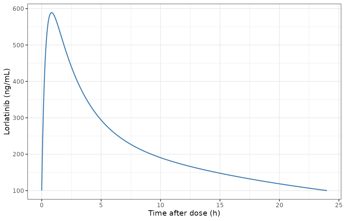
Simulated steady-state lorlatinib plasma profile over the last dosing interval of a 30-day 100 mg once-daily regimen.
Virtual population
Braniff 2025 generates plausible patients by sampling the Table S1 parameters and the Table S3 tumor physiology, enforcing three constraints (left box of Figure 2 and Supplement S2):
-
rho_core > 4 * tau * kg0, so the derived elimination ratekeis positive. When violated,rho_coreis re-drawn uniformly on[4 * tau * kg0, 0.75]; if that lower bound exceeds 0.75 the whole parameter set is rejected. -
phi_n0drawn uniformly on[phi_n0_min, 1], which guarantees no spontaneous shrinkage immediately after initialisation. - Untreated doubling time over a six-week simulation inside 26-165 days.
The plausible patients are then scored by a Metropolis-Hastings step and subsampled by acceptance-rejection against a Gaussian mixture fit to the observed clinical data. That selection step cannot be reproduced here: it requires the patient-level SLD and dropout data of Solomon 2018, which are not public. What follows is therefore the plausible population - constraints enforced, no clinical scoring - compared against the published virtual population.
n_candidates <- 500

# Draw uniformly within each published range.
cand <- as.data.frame(lapply(
  stats::setNames(seq_len(nrow(vpop_ranges)), vpop_ranges$parameter),
  function(i) stats::runif(n_candidates, vpop_ranges$lo[i], vpop_ranges$hi[i])
))

# Constraint 1: rho_core > 4 * tau * kg0.
rho_min <- 4 * cand$tau_necrotic * cand$kg0
cand    <- cand[rho_min < 0.75, ]
rho_min <- rho_min[rho_min < 0.75]
cand$rho_core <- stats::runif(nrow(cand), pmax(rho_min, 0.15), 0.75)

# Constraint 2: phi_n0 on [phi_n0_min, 1].
np0    <- (cand$delta_shell / rad_const)^3 /
          ((1 + cand$rho_core)^(1 / 3) - cand$rho_core^(1 / 3))^3
nn_tot <- cand$rho_core * np0
cand$phi_n0 <- stats::runif(
  nrow(cand),
  pmax(1 - 4 * cand$kg0 * cand$tau_necrotic * np0 / nn_tot, 0),
  1
)
cand$id <- seq_len(nrow(cand))

# The model file parameterises the sampled quantities on the log scale.
vpop_params <- cand
for (nm in vpop_ranges$parameter) {
  vpop_params[[paste0("l", nm)]] <- log(vpop_params[[nm]])
  vpop_params[[nm]] <- NULL
}
# Constraint 3: untreated doubling time within 26-165 days.
untreated <- rxode2::rxSolve(
  ui, make_events(seq(0, 42, by = 1), ids = vpop_params$id, dose = 0),
  params = vpop_params, atol = 1e-8, rtol = 1e-8, maxsteps = 1e5
) |>
  as.data.frame() |>
  dplyr::filter(!is.na(sld))
#> Warning: multi-subject simulation without without 'omega'

screen <- untreated |>
  dplyr::group_by(id) |>
  dplyr::summarise(
    td = 42 * log(2) / log((dplyr::last(sld) / dplyr::first(sld))^3),
    .groups = "drop"
  ) |>
  dplyr::filter(is.finite(td), td >= 26, td <= 165)

# Cap the cohort at the 155 virtual patients Braniff 2025 uses in Figures 4-5.
cohort <- vpop_params |>
  dplyr::filter(id %in% screen$id) |>
  head(155)

sprintf(
  "%d candidates drawn; %d passed the feasibility constraint; %d passed the Table S3 doubling-time gate; %d carried forward.",
  n_candidates, nrow(cand), nrow(screen), nrow(cohort)
)
#> [1] "500 candidates drawn; 187 passed the feasibility constraint; 147 passed the Table S3 doubling-time gate; 147 carried forward."
# Strong responders drive the tumor states down by several orders of
# magnitude, which needs tighter tolerances than the reference-patient
# solves; at atol/rtol = 1e-8 roughly a fifth of the cohort fails to solve.
vpop_sim <- rxode2::rxSolve(
  ui, make_events(seq(0, 500, by = 7), ids = cohort$id),
  params = cohort, atol = 1e-10, rtol = 1e-10, maxsteps = 1e6
) |>
  as.data.frame() |>
  dplyr::filter(!is.na(sld))
#> Warning: multi-subject simulation without without 'omega'

n_failed <- nrow(cohort) - dplyr::n_distinct(vpop_sim$id)

vpop_summary <- vpop_sim |>
  dplyr::group_by(id) |>
  dplyr::mutate(pct_change = 100 * (sld - dplyr::first(sld)) / dplyr::first(sld)) |>
  dplyr::summarise(
    baseline_sld = dplyr::first(sld),
    best_pct     = min(pct_change),
    .groups      = "drop"
  )

sprintf("%d of %d cohort members solved; %d dropped as unsolvable.",
        nrow(vpop_summary), nrow(cohort), n_failed)
#> [1] "147 of 147 cohort members solved; 0 dropped as unsolvable."
knitr::kable(
  tibble::tibble(
    `Endpoint` = c("Baseline SLD, median (mm)",
                   "Best % change, median",
                   "Responders (best % change < -30%)",
                   "Progressors (best % change > +20%)"),
    `Simulated plausible population` = c(
      sprintf("%.0f (IQR %.0f-%.0f)", median(vpop_summary$baseline_sld),
              quantile(vpop_summary$baseline_sld, 0.25),
              quantile(vpop_summary$baseline_sld, 0.75)),
      sprintf("%+.0f%%", median(vpop_summary$best_pct)),
      sprintf("%.0f%%", 100 * mean(vpop_summary$best_pct < -30)),
      sprintf("%.0f%%", 100 * mean(vpop_summary$best_pct > 20))
    ),
    `Braniff 2025 Figure 4` = c("bulk 20-150, centred near 50",
                                "about -45%", "about 65%", "about 5%")
  ),
  caption = paste(
    "Simulated plausible population vs the published virtual population.",
    "The simulated column omits the Metropolis-Hastings scoring and",
    "acceptance-rejection selection steps, which require the unavailable",
    "patient-level clinical data and shift the distribution toward the",
    "observed endpoints."
  )
)| Endpoint | Simulated plausible population | Braniff 2025 Figure 4 |
|---|---|---|
| Baseline SLD, median (mm) | 51 (IQR 26-69) | bulk 20-150, centred near 50 |
| Best % change, median | -15% | about -45% |
| Responders (best % change < -30%) | 45% | about 65% |
| Progressors (best % change > +20%) | 0% | about 5% |
vpop_summary |>
  dplyr::arrange(dplyr::desc(best_pct)) |>
  dplyr::mutate(pct_rank = 100 * (dplyr::row_number() - 0.5) / dplyr::n()) |>
  ggplot(aes(pct_rank, best_pct)) +
  geom_col(width = 0.9, fill = "firebrick") +
  geom_hline(yintercept = c(20, -30), linetype = "dashed", colour = "grey30") +
  labs(x = "Population percentile (%)", y = "Best change in SLD (%)") +
  theme_bw()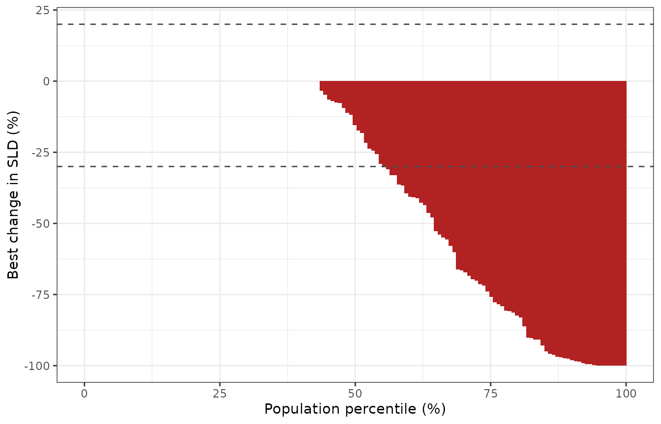
Waterfall plot of best percentage change in SLD for the simulated plausible population. Replicates the waterfall panel of Braniff 2025 Figure 4b; dashed lines are the RECIST +20% progression and -30% partial-response thresholds.
vpop_traj <- vpop_sim |>
  dplyr::group_by(id) |>
  dplyr::mutate(pct_change = 100 * (sld - dplyr::first(sld)) / dplyr::first(sld)) |>
  dplyr::ungroup()

vpop_band <- vpop_traj |>
  dplyr::group_by(time) |>
  dplyr::summarise(
    med = median(pct_change),
    lo  = quantile(pct_change, 0.25),
    hi  = quantile(pct_change, 0.75),
    .groups = "drop"
  )

ggplot() +
  geom_line(data = vpop_traj,
            aes(time / 7, pct_change, group = id),
            colour = "grey80", linewidth = 0.2) +
  geom_ribbon(data = vpop_band, aes(time / 7, ymin = lo, ymax = hi),
              fill = "firebrick", alpha = 0.25) +
  geom_line(data = vpop_band, aes(time / 7, med),
            colour = "firebrick", linewidth = 0.9) +
  geom_hline(yintercept = c(20, -30), linetype = "dashed", colour = "grey30") +
  coord_cartesian(ylim = c(-100, 60)) +
  labs(x = "Time (weeks)", y = "Change in SLD from baseline (%)") +
  theme_bw()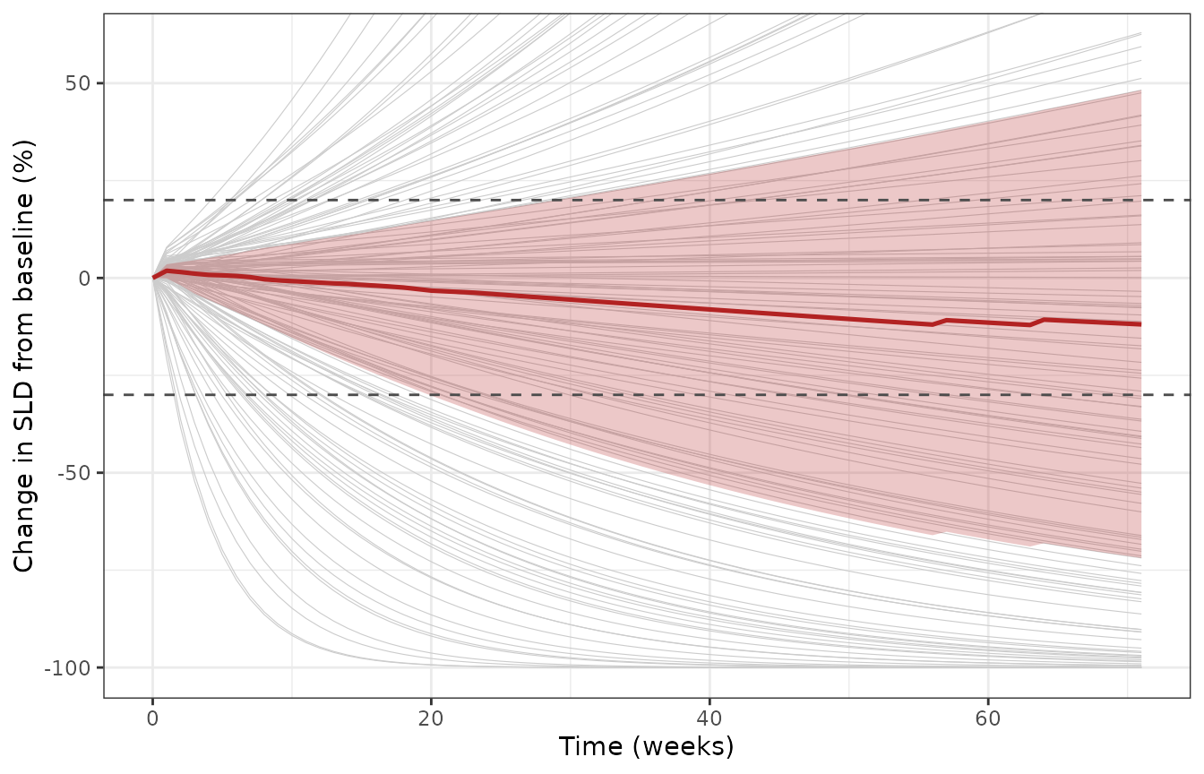
Median and interquartile range of percentage change in SLD over time for the simulated plausible population, with individual trajectories behind. Replicates the median-SLD panel of Braniff 2025 Figure 4b.
ggplot(vpop_summary, aes(baseline_sld)) +
  geom_histogram(bins = 25, fill = "steelblue", colour = "white") +
  scale_x_log10() +
  labs(x = "Baseline SLD (mm, log scale)", y = "Virtual patients") +
  theme_bw()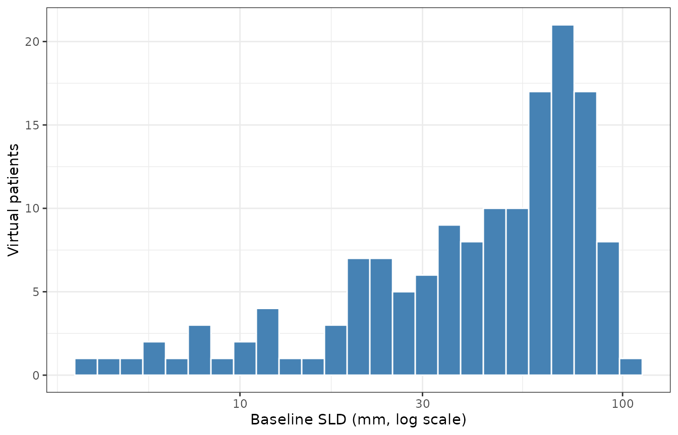
Distribution of baseline SLD in the simulated plausible population. Braniff 2025 Figure 4a plots the observed baseline SLD on a logarithmic axis spanning 5-500 mm, with the fitted mixture centred near 50 mm.
Assumptions and deviations
The paper reports no point estimates. Braniff 2025
is a virtual-population methodology paper. Tables S1 and S3 give
sampling ranges for the eleven quantities the algorithm
samples; there are no published point estimates, and none are implied.
The ini() values are a single reference plausible patient
obtained by digitising the published marginal distributions - Figure 6a
for gfr_act, delta_shell,
hill_prolif (alpha) and kg0, which plots
responder/non-responder quartiles on a “% value between feasible bounds”
axis, and Figure S2 for the other seven. The pooled median for the
Figure 6a parameters is approximated as
0.65 * responder + 0.35 * non-responder, the responder
fraction read from the Figure 4b waterfall. Digitisation precision is
about +/- 5 percentage points of each range. These are not
published estimates and must not be cited as such. The
reference patient is a strong responder; the population-level endpoints
are validated above by sampling the published ranges, which is the
paper’s own construction.
Reading of the shell-to-core transfer rate
kn. As shown above, the literal reading of the
printed kn equation (with rho_core as the
core-shell ratio) does not hold the core-shell ratio constant as the
surrounding text states it does, cannot reach the Table S3
untreated-growth window anywhere in the published parameter space, and
produces essentially static tumors. Reading rho_core in
that one equation as the necrotic fraction
phi_n = rho_core / (1 + rho_core) makes the printed
expression algebraically identical to the ratio-preserving rate,
satisfies Table S3, and reproduces Figure 4b. The fraction reading is
adopted. Note that the supplement uses both symbols - Section S2 defines
phi_n = rho_core / (1 + rho_core) and works with it
throughout - so this is a symbol-overloading slip rather than an error
in the underlying model.
Dimensional constant in the tumor geometry. The
supplement’s expression for Np in terms of
delta_shell equates a length cubed with a cell count; the
dimensional constant is omitted as printed. It is recovered from the
supplement’s own statement that there are 1e5 cells per microlitre, plus
the spherical geometry the Figure 1 caption specifies: a cell count
n occupies n * 1e-5 mm^3, so the equivalent
sphere has radius (3 * n * 1e-5 / (4 * pi))^(1/3). The
reconstruction is checked independently by the virtual-population
baseline SLD distribution above, which lands where Figure 4a puts the
observed distribution.
Molar-unit conversion. Braniff Table S1 reports
IC50 in nM while the PK model returns mg/L. The conversion
uses the molar mass of lorlatinib (406.41 g/mol, C21H19FN6O2), which is
a physical constant of the compound and not a Braniff parameter. Without
a conversion the drug would sit three orders of magnitude below its own
IC50 and produce no effect at all, so the molar reading is the only
self-consistent one.
Zero-order absorption duration D1.
Supplement S1 describes “sequential zero and first order absorption” but
Table S2 tabulates no D1. The value 1.148 h is inherited
from the PK source the supplement cites for the whole PK block (Chen
2021), as extracted in
inst/modeldb/specificDrugs/Chen_2021_lorlatinib.R. This is
the only parameter in the file that is not in Braniff’s own tables. It
has no effect on steady-state exposure and, given
ka = 74.7 1/day, very little on the profile shape.
Clearance at time zero. Braniff’s
CL(t) = CLmax * (1 - exp(-kc * t)) starts at
CL = 0, whereas the Chen 2021 model it is derived from
starts at a single-dose CLI = 9.035 L/h; Braniff Table S2
tabulates no CLI. The printed form is encoded as-is. The
consequence is confined to the first days of dosing: simulated day-1
AUC0-24 is about 26% higher than the steady-state AUC0-tau, whereas the
Chen parameterisation gives a day-1 AUC below steady state. Steady-state
exposure is unaffected because both forms converge to
CLmax, and the signaling model is driven by the median
steady-state profile.
No residual error and no IIV. Braniff 2025 fits no
residual-error model and carries no random effects; the QSP model is
deterministic and all variability is generated by parameter sampling.
Both endpoints therefore carry fixed(0) residual SDs rather
than invented variances.
Numerical guards. max(ps6, 0) and
max(1 - pakt, 0) are numerical guards only. Both quantities
are non-negative for every admissible trajectory, but a round-off-sized
negative value raised to a non-integer Hill exponent returns
NaN and aborts the solve. The clamps change no admissible
trajectory.
Selection step not reproduced. The Metropolis-Hastings scoring, the dropout-time resampling and censoring assignment, and the acceptance-rejection subsampling all require the patient-level SLD and dropout data from Solomon 2018, which are not public. The virtual-population section above therefore reproduces the plausible population only. The consequences are visible in the comparison table: the simulated best-percentage-change distribution is less deeply negative than the published virtual population, and the simulated population contains no RECIST progressors, because progression in the trial also arises from new lesions and non-target growth, which Braniff handles in the dropout-resampling step rather than in the ODE model.
Progression-free survival is not modelled here. PFS in Braniff 2025 is not an output of the ODE system; it is assigned by resampling observed dropout times and censoring labels during the selection algorithm. It therefore cannot be reproduced from the model file alone and is out of scope for this vignette.