Acute hepatitis B virus infection QSP model (Boivin-Champeaux 2026)
Source:vignettes/articles/BoivinChampeaux_2026_hepatitisB_qsp.Rmd
BoivinChampeaux_2026_hepatitisB_qsp.RmdModel and source
- Citation: Boivin-Champeaux C, Schmidt S, Balsitis S, Johansson Azeredo F, Feigelman JS. A Quantitative Systems Pharmacology (QSP) Model of Acute Hepatitis B Virus Infection: Mechanistic Insights and Foundations for Future Extensions. CPT Pharmacometrics Syst Pharmacol. 2026;15(2):e70172. doi:10.1002/psp4.70172. Model equations from Supplementary Material 2 (Eq. S1-S89); parameter values, initial conditions and the repeated-assignment rules from Supplementary Material 3 (Table S3: Parameter values, Table S4: Initial conditions, Table S4: Repeated Assignments); model-building narrative, generic regulatory forms (Table S1) and the uninfected steady-state verification (Table S2) from Supplementary Material 1. Includes the publisher correction of 14 January 2026 (InSysBio location corrected to the UK), which does not alter any value.
- Article: https://doi.org/10.1002/psp4.70172
Boivin-Champeaux and colleagues (CPT: Pharmacometrics & Systems Pharmacology, 2026) describe a multiscale quantitative systems pharmacology (QSP) model of acute hepatitis B virus (HBV) infection. The model spans three anatomical compartments – liver, plasma and lymph node – and five mechanistic modules: the viral life cycle, the innate immune system, the adaptive immune system, cytokine signalling, and the mechanisms of viral clearance. It was built in MATLAB SimBiology, comprises 98 species and 319 parameters, and was calibrated by hand against digitised biomarker time courses from eight published acute-HBV cohorts.
This is a typical-individual, deterministic mechanism model. It has no IIV and no residual-error model: the authors state that the model’s size and the sparseness of acute-HBV data prevented convergence of automated estimation, so 45 remaining parameters were calibrated manually. The published population-level variability is a virtual population produced by Markov-chain resampling of the 23 most influential parameters (Appendix S4, Table S5), not an omega matrix. Accordingly this vignette validates the model the way the endogenous / mechanistic model class demands – steady state, perturbation recovery, flux balance and dimensional consistency – rather than by non-compartmental analysis. There is no drug, no dose and no absorption-distribution-elimination profile for PKNCA to integrate.
mod <- readModelDb("BoivinChampeaux_2026_hepatitisB_qsp")
ui  <- rxode2::rxode2(mod)

c(states = length(ui$state), parameters = length(ui$theta))
#>     states parameters
#>         89        324
Infection is initiated purely through the parameter
HBV0, the plasma HBV inoculum. HBV0 = 0 gives
the uninfected subject; HBV0 = 0.333 virion/mL (1000 HBV
DNA copies distributed through 3000 mL of plasma, a needle-stick
exposure) gives the acute infection the paper simulates.
# The system spans rate constants from 0 (drainage) to 214/day (IL-6) and
# states from 0 to 1.6e8 cell/mL, so it is stiff. Tight tolerances are
# required for the uninfected steady-state assertions below to be meaningful.
solve_hbv <- function(hbv0 = 0.333, times = seq(0, 450, by = 1), ...) {
  rxode2::rxSolve(
    ui,
    rxode2::et(times),
    params     = c(HBV0 = hbv0, ...),
    returnType = "data.frame",
    atol       = 1e-10,
    rtol       = 1e-8
  )
}
Population
pop <- ui$population
tibble::tibble(Field = names(pop), Value = vapply(pop, paste, character(1), collapse = "; ")) |>
knitr::kable()| Field | Value |
|---|---|
| species | human |
| n_subjects | 71 |
| n_studies | 8 |
| age_range | adults; not systematically reported across the eight source cohorts |
| disease_state | Acute hepatitis B virus infection in immunocompetent adults, predominantly self-limiting. One subject in Webster et al. (Patient 5) and one in Kuhns et al. progressed to persistent infection; Patient 5 was treated as an outlier and excluded from the virtual-population comparison. |
| dose_range | No drug. Infection is initiated by an HBV inoculum of 1000 HBV DNA copies distributed in 3000 mL plasma (0.333 virion/mL), consistent with a needle-stick exposure (SM1 section 1). |
| notes | Calibration data were digitised (Graph Grabber v2.0.2) from eight published acute-HBV cohorts (Table 1): Webster 2000 (n = 5), Whalley 2001 (n = 7), Chulanov 2003 (n = 21), Fisicaro 2009 (n = 2), Dunn 2009 (n = 9), Okamoto 2019 (n = 1), Kuhns 2021 (n = 5), Panduro 2022 (n = 1); Whalley patients 1-5 overlap with Webster, so n_subjects = 71 counts the reported per-study cohort sizes. Because infection onset was rarely reported, each study’s time axis was shifted to days-post-infection using the per-study rules in SM1 Table S3. Model parameters were taken from peer-reviewed literature and from InSysBio (UK) CYTOCON DB, fIVE DB and the Immune Response Template; 45 parameters remained to be estimated and were hand-calibrated. There is no observed-subject-level parameter distribution: the published virtual population (20,000 Markov chain samples of the 23 most influential parameters, filtered against binned clinical percentiles) is summarised in Appendix S4 Table S5 and is not reproduced as an omega matrix. |
The calibration data are digitised (Graph Grabber v2.0.2) biomarker time courses from the eight cohorts listed in Table 1 of the paper: Webster 2000 (n = 5), Whalley 2001 (n = 7), Chulanov 2003 (n = 21), Fisicaro 2009 (n = 2), Dunn 2009 (n = 9), Okamoto 2019 (n = 1), Kuhns 2021 (n = 5) and Panduro 2022 (n = 1). Because infection onset was rarely reported, each study’s time axis was shifted to days-post-infection using the per-study rules in SM1 Table S3 (for example, Chulanov’s “days after first symptomatic day” were shifted by the 105-day mean incubation period).
Source trace
Every equation and every parameter value in the model file is traceable to one of the four supplementary appendices. The appendix files are numbered independently of the “Supplementary Material” (SM) sections they contain:
| Appendix file | Contains |
|---|---|
| Appendix S3 | SM1: model building narrative, Table S1 (generic regulatory forms), Table S2 (uninfected steady-state verification), Table S3 (time-adjustment strategy) |
| Appendix S2 | SM2: all model equations, Eq. S1-S89 |
| Appendix S1 | SM3: Table S4 (initial conditions for volumes and species), Table S3 (parameter values), Table S4 (repeated assignments) |
| Appendix S4 | SM4: Table S5 (virtual-population parameter distributions) |
| Model element | Source |
|---|---|
| 89 ODE states | SM2 Eq. S1-S89 (liver S1-S29, plasma S30-S53, lymph S54-S89) |
| 34 repeated-assignment rules | SM3 “Table S4: Repeated Assignments” |
9 algebraic species (NK_TRAIL_LV,
CD8_IFNg_LV, HBsAg_PL, HBV_nM_PL,
HBV_DNA_IU, HBsAg_IU,
antiHBs_mIU, antiHBe_mIU,
antiHBc_mIU) |
SM3 Table S4, Notes column |
| 319 parameter values | SM3 “Table S3: Parameter values” |
| 89 initial conditions and 3 volumes | SM3 “Table S4: Initial conditions” |
Inoculum HBV0 = 0.333 virion/mL |
SM1 section 1 |
| Generic activation / inhibition forms | SM1 section 2, Table S1 |
The volume convention
Every equation in SM2 is written in the SimBiology rate-rule form
so intra-compartment terms reduce to rate_i and
inter-compartment terms carry the volume ratio
V_source / V_target. That reading is not assumed – it is
confirmed below against twelve independent baseline values that SM1
Table S2 reports, several of which are sensitive to the ratio. For
example, liver IL-10 balances against plasma IL-10 only if the influx
term carries V_PL / V_LV = 2:
# Symbolic check of the liver/plasma IL-10 pair (Eq. S25 and Eq. S53) at the
# uninfected baseline, where the only IL-10 source is naive mDC in the liver.
th <- setNames(ui$theta, names(ui$theta))
prod_IL10 <- th[["kprod_IL10_mDCnaive"]] * 1.92e4              # pg/mL/day
# Eq. S53 steady state: IL10_PL = kLV_PL_IL10 * (V_LV/V_PL) / kPL_LV_IL10 * IL10_LV
ratio_PL_LV <- th[["kLV_PL_IL10"]] * (th[["V_LV"]] / th[["V_PL"]]) / th[["kPL_LV_IL10"]]
# Eq. S25 steady state, substituting IL10_PL:
loss  <- th[["kdeg_IL10"]] + th[["kLV_PL_IL10"]] + th[["kdrain_IL10"]]
recyc <- th[["kPL_LV_IL10"]] * ratio_PL_LV * (th[["V_PL"]] / th[["V_LV"]])
IL10_LV_ss <- prod_IL10 / (loss - recyc)
c(IL10_LV_predicted = IL10_LV_ss,
  IL10_LV_tableS2   = 4.824,
  IL10_PL_predicted = ratio_PL_LV * IL10_LV_ss,
  IL10_PL_tableS2   = 1.500)
#> IL10_LV_predicted   IL10_LV_tableS2 IL10_PL_predicted   IL10_PL_tableS2
#>          4.823999          4.824000          1.500000          1.500000
stopifnot(
  isTRUE(all.equal(IL10_LV_ss,               4.824, tolerance = 1e-4)),
  isTRUE(all.equal(ratio_PL_LV * IL10_LV_ss, 1.500, tolerance = 1e-4))
)
Both reproduce SM1 Table S2 to four significant figures, which pins
the volume convention, kdrain_IL10,
kPL_LV_IL10 and kprod_IL10_mDCnaive
simultaneously.
Units
The model’s time unit is days throughout. Every ODE is a
concentration balance, so each right-hand-side term must carry
[state units] / day.
| Symbol class | Units | Example term | Units check |
|---|---|---|---|
| Cell states | cell/mL | kdeath_Hep * Hep_LV |
(1/day)(cell/mL) = cell/mL/day |
| Virion / particle states | virion/mL, item/mL | ksyn_HBV_cccDNA * iHep1_LV |
(virion/cell/day)(cell/mL) = virion/mL/day |
| Cytokine states | pg/mL | kprod_IL6_KCnaive * KCn_LV |
(pg/cell/day)(cell/mL) = pg/mL/day |
| Antigen / antibody states | IU/mL, molecule/mL | kon_antiHBc * HBcAg_PL * antiHBc_PL |
(mL/molecule/day)(molecule/mL)(molecule/mL) = molecule/mL/day |
| Inter-compartment transfer | 1/day, times a volume ratio | kPL_LV_NK * NKn_PL * (V_PL / V_LV) |
(1/day)(cell/mL)(1) = cell/mL/day |
| Lysis rates | cell/day (absolute) | NK_lysis_rate_Hep / V_LV |
(cell/day)/(mL) = cell/mL/day |
| Hill / Emax / Imax factors | dimensionless | 1 + Emax_IL12_Th1act * IL12_LV / (EC50 + IL12_LV) |
dimensionless |
| Slope factors | mL/pg | 1 + SLP_IFNg_TNFa * IFNg_LV |
1 + (mL/pg)(pg/mL) = dimensionless |
Three unit conversions are worth calling out, all from SM3 Table S4 Notes:
-
HBV_DNA_IU = HBV_PL * 0.2– one copy is one virion and the HBV DNA conversion factor is 0.2 IU/copy. -
HBsAg_IU = (HBV_PL + SVP_PL) / 5e7– from the WHO reference standard, 1 IU/mL of HBsAg corresponds to 5e7 particles. -
antiHBs_mIU = antiHBs_PL * 2.7e-16 * 13.43 * 1e3– molecules/mL to mIU/mL. The same2.7e-16 * 13.43factor appears inside Eq. S44 itself, converting the anti-HBe plasma-cell production term from molecules to IU.
Two published terms are dimensionally inconsistent as printed and are transcribed unchanged; both are discussed under Errata below.
Parameter table
The 319 tabulated parameters are too many to list here, so the table below shows the model file against SM3 Table S3 for the parameters the paper’s own local sensitivity analysis (Figure 5) ranked as most influential.
lsa_params <- c(
  "k_cccDNA_inc", "k_HBV_intern", "NTCP", "KD_HBV", "f_cccDNA",
  "kdeg_HBV_LV", "kdeg_HBV_PL", "kLV_PL_HBV", "f_liver_vasc", "kdeath_iHep",
  "kprol_PB", "kdeath_plasmablasts", "Emax_IL4_PBprol", "Emax_IL21_PBdiff",
  "kdeath_Bnaive_LN", "EC50_IL4_PBprol", "kprod_Ab_HBs", "n_PB", "MTT_PB",
  "kdiff_CD8_LN", "kdeath_eCD8", "n_HBV_mDC", "MAX_Hep_LV"
)
published <- c(
  k_cccDNA_inc = 0.0024, k_HBV_intern = 7.33, NTCP = 225, KD_HBV = 450,
  f_cccDNA = 0.99, kdeg_HBV_LV = 0.67, kdeg_HBV_PL = 0.67, kLV_PL_HBV = 1,
  f_liver_vasc = 0.15, kdeath_iHep = 0.062, kprol_PB = 0.3333,
  kdeath_plasmablasts = 0.2518, Emax_IL4_PBprol = 1.8, Emax_IL21_PBdiff = 1.5,
  kdeath_Bnaive_LN = 0.2, EC50_IL4_PBprol = 20, kprod_Ab_HBs = 1.5e6,
  n_PB = 2, MTT_PB = 9.5, kdiff_CD8_LN = 0.0012, kdeath_eCD8 = 0.03,
  n_HBV_mDC = 1.2, MAX_Hep_LV = 1.6e8
)
ptab <- tibble::tibble(
  Parameter          = lsa_params,
  `SM3 Table S3`     = published[lsa_params],
  `Model file`       = ui$theta[lsa_params]
)
knitr::kable(ptab)| Parameter | SM3 Table S3 | Model file |
|---|---|---|
| k_cccDNA_inc | 2.400e-03 | 2.400e-03 |
| k_HBV_intern | 7.330e+00 | 7.330e+00 |
| NTCP | 2.250e+02 | 2.250e+02 |
| KD_HBV | 4.500e+02 | 4.500e+02 |
| f_cccDNA | 9.900e-01 | 9.900e-01 |
| kdeg_HBV_LV | 6.700e-01 | 6.700e-01 |
| kdeg_HBV_PL | 6.700e-01 | 6.700e-01 |
| kLV_PL_HBV | 1.000e+00 | 1.000e+00 |
| f_liver_vasc | 1.500e-01 | 1.500e-01 |
| kdeath_iHep | 6.200e-02 | 6.200e-02 |
| kprol_PB | 3.333e-01 | 3.333e-01 |
| kdeath_plasmablasts | 2.518e-01 | 2.518e-01 |
| Emax_IL4_PBprol | 1.800e+00 | 1.800e+00 |
| Emax_IL21_PBdiff | 1.500e+00 | 1.500e+00 |
| kdeath_Bnaive_LN | 2.000e-01 | 2.000e-01 |
| EC50_IL4_PBprol | 2.000e+01 | 2.000e+01 |
| kprod_Ab_HBs | 1.500e+06 | 1.500e+06 |
| n_PB | 2.000e+00 | 2.000e+00 |
| MTT_PB | 9.500e+00 | 9.500e+00 |
| kdiff_CD8_LN | 1.200e-03 | 1.200e-03 |
| kdeath_eCD8 | 3.000e-02 | 3.000e-02 |
| n_HBV_mDC | 1.200e+00 | 1.200e+00 |
| MAX_Hep_LV | 1.600e+08 | 1.600e+08 |
Every one of the 23 most influential published values is carried in
the model file exactly; the stopifnot() above is an
enumerating check, so adding a parameter to lsa_params
without adding it to published fails the render.
Validation 1: uninfected steady state
SM1 Table S2 reports the concentration of every species at
t = 0 and at t = 450 days under uninfected
baseline conditions, and asserts that all of them are at steady state.
This is the strongest single check available on the transcription,
because it exercises every homeostatic term simultaneously.
ss <- solve_hbv(hbv0 = 0, times = seq(0, 450, by = 10))

tableS2 <- tibble::tribble(
  ~species,     ~compartment, ~tableS2,
  "Hep_LV",     "Liver",      1.60e8,
  "KCn_LV",     "Liver",      3.70e7,
  "NKn_LV",     "Liver",      1.46e5,
  "NKbr_LV",    "Liver",      3.88e4,
  "NKdim_LV",   "Liver",      8.74e4,
  "mDCn_LV",    "Liver",      1.92e4,
  "TGFb_LV",    "Liver",      45.000,
  "IL10_LV",    "Liver",      4.824,
  "IL6_LV",     "Liver",      5.000,
  "NKn_PL",     "Plasma",     3.00e5,
  "pDCn_PL",    "Plasma",     1.32e4,
  "mDCn_PL",    "Plasma",     2.40e4,
  "IL10_PL",    "Plasma",     1.500,
  "ALT_PL",     "Plasma",     0.030,
  "CD8n_LN",    "Lymph",      5.00e7,
  "CD4n_LN",    "Lymph",      9.00e7,
  "BnHBs_LN",   "Lymph",      1.50e4,
  "BnHBe_LN",   "Lymph",      1.50e4,
  "BnHBc_LN",   "Lymph",      1.50e4,
  "TGFb_LN",    "Lymph",      10.000,
  "IL6_LN",     "Lymph",      15.420,
  "IL10_LN",    "Lymph",      0.420
)

ss_cmp <- tableS2 |>
  mutate(
    # unname(): vapply() carries the species names through, and a named
    # vector never compares equal to an unnamed one under all.equal().
    sim_t0   = unname(vapply(species, function(s) ss[[s]][1], numeric(1))),
    sim_t450 = unname(vapply(species, function(s) ss[[s]][nrow(ss)], numeric(1))),
    `drift %` = 100 * (sim_t450 - tableS2) / tableS2
  )
knitr::kable(ss_cmp, digits = c(0, 0, 4, 4, 4, 3))| species | compartment | tableS2 | sim_t0 | sim_t450 | drift % |
|---|---|---|---|---|---|
| Hep_LV | Liver | 1.600e+08 | 1.6000e+08 | 1.596600e+08 | -0.213 |
| KCn_LV | Liver | 3.700e+07 | 3.7000e+07 | 3.997167e+07 | 8.032 |
| NKn_LV | Liver | 1.460e+05 | 1.4600e+05 | 1.459351e+05 | -0.044 |
| NKbr_LV | Liver | 3.880e+04 | 3.8800e+04 | 3.879647e+04 | -0.009 |
| NKdim_LV | Liver | 8.740e+04 | 8.7387e+04 | 8.737944e+04 | -0.024 |
| mDCn_LV | Liver | 1.920e+04 | 1.9200e+04 | 1.920000e+04 | 0.000 |
| TGFb_LV | Liver | 4.500e+01 | 4.5000e+01 | 4.500000e+01 | 0.000 |
| IL10_LV | Liver | 4.824e+00 | 4.8240e+00 | 4.824000e+00 | 0.000 |
| IL6_LV | Liver | 5.000e+00 | 5.0000e+00 | 5.402800e+00 | 8.056 |
| NKn_PL | Plasma | 3.000e+05 | 3.0000e+05 | 3.000506e+05 | 0.017 |
| pDCn_PL | Plasma | 1.320e+04 | 1.3200e+04 | 1.320000e+04 | 0.000 |
| mDCn_PL | Plasma | 2.400e+04 | 2.4000e+04 | 2.400000e+04 | 0.000 |
| IL10_PL | Plasma | 1.500e+00 | 1.5000e+00 | 1.500000e+00 | 0.000 |
| ALT_PL | Plasma | 3.000e-02 | 3.0000e-02 | 2.990000e-02 | -0.211 |
| CD8n_LN | Lymph | 5.000e+07 | 5.0000e+07 | 5.000000e+07 | 0.000 |
| CD4n_LN | Lymph | 9.000e+07 | 9.0000e+07 | 9.000000e+07 | 0.000 |
| BnHBs_LN | Lymph | 1.500e+04 | 1.5000e+04 | 1.500000e+04 | 0.000 |
| BnHBe_LN | Lymph | 1.500e+04 | 1.5000e+04 | 1.500000e+04 | 0.000 |
| BnHBc_LN | Lymph | 1.500e+04 | 1.5000e+04 | 1.500000e+04 | 0.000 |
| TGFb_LN | Lymph | 1.000e+01 | 1.0000e+01 | 9.999500e+00 | -0.005 |
| IL6_LN | Lymph | 1.542e+01 | 1.5420e+01 | 1.666220e+01 | 8.056 |
| IL10_LN | Lymph | 4.200e-01 | 4.2000e-01 | 4.200000e-01 | 0.008 |
Every initial condition matches SM1 Table S2 exactly, and 19 of the 22 species hold that value over 450 simulated days to better than 0.25 %:
holds <- ss_cmp |> filter(!species %in% c("KCn_LV", "IL6_LV", "IL6_LN"))
ic_rel <- abs(ss_cmp$sim_t0 - ss_cmp$tableS2) / ss_cmp$tableS2
stopifnot(
  # Initial conditions reproduce Table S2 at t = 0. The single non-zero
  # residual is NKdim_LV, where Table S2 rounds the Table S4 initial
  # assignment 8.7387e4 to 8.74e4.
  nrow(ss_cmp) == 22L,
  max(ic_rel) < 2e-4,
  sum(ic_rel > 0) == 1L,
  ss_cmp$species[which.max(ic_rel)] == "NKdim_LV",
  # 19 of 22 species hold that value to < 0.25 % over 450 days
  nrow(holds) == 19L,
  max(abs(holds$`drift %`)) < 0.25
)
c(`max initial-condition relative error` = max(ic_rel),
  `max drift %, 19 holding species`      = max(abs(holds$`drift %`)))
#> max initial-condition relative error      max drift %, 19 holding species
#>                         0.0001487414                         0.2125000001
The three drifting species have one root cause
KCn_LV, IL6_LV and IL6_LN all
drift by the same +8.0 %. The cause is arithmetic, not a transcription
error: SM3 Table S4 gives the naive Kupffer cell baseline as 3.7e7
cell/mL, but the tabulated kprol_KC,
kdeath_KCnaive and MAX_KC_LV put the logistic
fixed point of Eq. S6 elsewhere. Liver IL-6 is produced by naive Kupffer
cells (Eq. S26) and lymph IL-6 is fed by liver drainage (Eq. S87), so
both inherit the same offset.
kc_fixed_point <- th[["MAX_KC_LV"]] * (1 - th[["kdeath_KCnaive"]] / th[["kprol_KC"]])
c(`Table S4 baseline`   = 3.70e7,
  `Eq. S6 fixed point`  = kc_fixed_point,
  `simulated t = 450`   = ss$KCn_LV[nrow(ss)],
  `offset %`            = 100 * (kc_fixed_point - 3.7e7) / 3.7e7)
#>  Table S4 baseline Eq. S6 fixed point  simulated t = 450           offset %
#>       3.700000e+07       3.997358e+07       3.997167e+07       8.036716e+00
# The simulated endpoint is the analytic fixed point of Eq. S6, not the
# tabulated baseline: the model is behaving correctly and the published
# parameter set is internally inconsistent by ~8 %.
drift_of <- function(sp) ss_cmp$`drift %`[ss_cmp$species == sp]
stopifnot(
  abs(ss$KCn_LV[nrow(ss)] - kc_fixed_point) / kc_fixed_point < 1e-3,
  # IL-6 in both liver and lymph tracks the Kupffer offset, not something else
  abs(drift_of("IL6_LV") - drift_of("KCn_LV")) < 0.05,
  abs(drift_of("IL6_LN") - drift_of("IL6_LV")) < 0.05
)
That the IL-6 drift equals the Kupffer drift to within 0.05 percentage points in both compartments confirms the single root cause and rules out an independent error in Eq. S26 or Eq. S87.
Validation 2: perturbation recovery
Displacing a homeostatic state and letting it relax confirms that the baseline is a genuine attractor rather than a value that merely happens to be written in the initial conditions.
The relaxation rates of the homeostatic pools span three orders of
magnitude, so the horizon has to be set by the slowest mode. The naive
CD4 pool in lymph turns over at kdeath_CD4naive_LN =
0.002/day (a 500-day time constant), which is by a wide margin the
slowest mode of the uninfected system, so the recovery runs are carried
out to 3500 days – seven time constants of that pool.
horizon <- 3500
recover <- function(state, factor) {
  ic <- setNames(ss[[state]][1] * factor, state)
  s  <- rxode2::rxSolve(
    ui, rxode2::et(seq(0, horizon, by = 10)), params = c(HBV0 = 0),
    inits = ic, returnType = "data.frame", atol = 1e-10, rtol = 1e-8
  )
  tibble::tibble(time = s$time, value = s[[state]], state = state,
                 start = paste0(factor, "x baseline"))
}
rec <- bind_rows(
  recover("TGFb_LV", 0.5), recover("TGFb_LV", 2),
  recover("IL10_PL", 0.5), recover("IL10_PL", 2),
  recover("NKn_PL",  0.5), recover("NKn_PL",  2),
  recover("CD4n_LN", 0.5), recover("CD4n_LN", 2)
)

ggplot(rec, aes(time, value, colour = start)) +
  geom_line() +
  facet_wrap(~state, scales = "free_y") +
  scale_x_continuous(trans = "log1p",
                     breaks = c(0, 1, 10, 100, 1000, 3500)) +
  labs(x = "Time (days, log1p scale)", y = "Concentration", colour = NULL,
       title = "Perturbation recovery to the uninfected baseline") +
  theme_bw()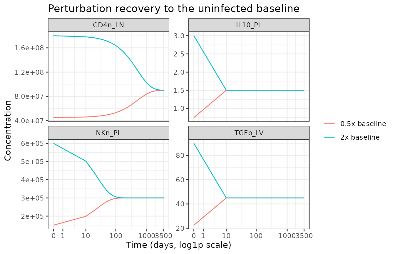
Each displaced state returns monotonically to its SM1 Table S2 baseline, at a rate that matches the analytic relaxation constant of its own balance equation.
baselines <- c(TGFb_LV = 45, IL10_PL = 1.5, NKn_PL = 3.0e5, CD4n_LN = 9.0e7)
# Analytic relaxation rate of each pool at the uninfected baseline.
rate <- c(
  TGFb_LV = th[["kdeg_TGFb"]] + th[["kdrain_TGFb"]],           # Eq. S24
  IL10_PL = th[["kPL_LV_IL10"]],                               # Eq. S53
  NKn_PL  = th[["kPL_LV_NK"]] + th[["kdeath_NKnaive"]],        # Eq. S35
  CD4n_LN = th[["kdeath_CD4naive_LN"]]                         # Eq. S57
)
final <- rec |>
  group_by(state, start) |>
  summarise(final = value[which.max(time)], .groups = "drop") |>
  mutate(
    target             = unname(baselines[state]),
    `rel. residual`    = abs(final - target) / target,
    `time constant (d)` = unname(1 / rate[state]),
    `horizon / tau`    = horizon * unname(rate[state])
  )
knitr::kable(final, digits = c(0, 0, 4, 4, 6, 1, 1))| state | start | final | target | rel. residual | time constant (d) | horizon / tau |
|---|---|---|---|---|---|---|
| CD4n_LN | 0.5x baseline | 89958965.3 | 9.0e+07 | 0.000456 | 500.0 | 7.0 |
| CD4n_LN | 2x baseline | 90082069.4 | 9.0e+07 | 0.000912 | 500.0 | 7.0 |
| IL10_PL | 0.5x baseline | 1.5 | 1.5e+00 | 0.000000 | 0.6 | 5628.0 |
| IL10_PL | 2x baseline | 1.5 | 1.5e+00 | 0.000000 | 0.6 | 5628.0 |
| NKn_PL | 0.5x baseline | 300050.6 | 3.0e+05 | 0.000169 | 25.3 | 138.2 |
| NKn_PL | 2x baseline | 300050.6 | 3.0e+05 | 0.000169 | 25.3 | 138.2 |
| TGFb_LV | 0.5x baseline | 45.0 | 4.5e+01 | 0.000000 | 0.4 | 7840.0 |
| TGFb_LV | 2x baseline | 45.0 | 4.5e+01 | 0.000000 | 0.4 | 7840.0 |
stopifnot(
  nrow(final) == 8L,
  # every pool is within 0.5 % of its Table S2 baseline at 3500 days
  all(final$`rel. residual` < 5e-3),
  # and the horizon really is many time constants for each of them
  all(final$`horizon / tau` > 6)
)
c(`max relative residual at 3500 d` = max(final$`rel. residual`))
#> max relative residual at 3500 d
#>                     0.000911882
Validation 3: flux balance
At the uninfected baseline, production and elimination must cancel term by term. Working the balances symbolically – rather than only observing that the simulation does not move – confirms that the equations are self-consistent and that the tabulated rate constants are the ones that make them so.
p <- function(x) th[[x]]
flux <- tibble::tribble(
  ~equation, ~species, ~predicted, ~tableS2,
  "S35", "NKn_PL",  p("ksyn_NK") / (p("kPL_LV_NK") + p("kdeath_NKnaive")),                 3.00e5,
  "S36", "pDCn_PL", p("ksyn_pDC") / p("kdeath_pDCnaive"),                                  1.32e4,
  "S38", "mDCn_PL", p("ksyn_mDC") / (p("kPL_LV_DC") + p("kdeath_mDCnaive")),               2.40e4,
  "S11", "mDCn_LV", p("kPL_LV_DC") * 2.4e4 * (p("V_PL") / p("V_LV")) / p("kdeath_mDCnaive"), 1.92e4,
  "S8",  "NKn_LV",  p("kPL_LV_NK") * 3.0e5 * (p("V_PL") / p("V_LV")) /
                      (p("kdeath_NKnaive") + p("kact_eff0")),                              1.46e5,
  "S9",  "NKbr_LV", p("kact_eff0") * 1.4591e5 / (p("kdeath_NKact") + p("kmature_NK_LV")),   3.88e4,
  "S10", "NKdim_LV", p("kmature_NK_LV") * 3.88e4 / p("kdeath_NKact"),                      8.74e4,
  "S55", "CD8n_LN", p("ksyn_CD8") / p("kdeath_CD8naive_LN"),                               5.00e7,
  "S57", "CD4n_LN", p("ksyn_CD4") / p("kdeath_CD4naive_LN"),                               9.00e7,
  "S62", "BnHBs_LN", p("ksyn_Bcell") / p("kdeath_Bnaive_LN"),                              1.50e4,
  "S24", "TGFb_LV", p("kprod_TGFb_mDCnaive") * 1.92e4 / (p("kdeg_TGFb") + p("kdrain_TGFb")), 45.000,
  "S85", "TGFb_LN", p("kdrain_TGFb") * 45 * (p("V_LV") / p("V_LN")) / p("kdeg_TGFb"),      10.000,
  "S26", "IL6_LV",  p("kprod_IL6_KCnaive") * 3.7e7 / (p("kdeg_IL6") + p("kdrain_IL6")),     5.000,
  "S87", "IL6_LN",  p("kdrain_IL6") * 5 * (p("V_LV") / p("V_LN")) / p("kdeg_IL6"),         15.420,
  "S89", "IL10_LN", p("kdrain_IL10") * 4.824 * (p("V_LV") / p("V_LN")) / p("kdeg_IL10"),    0.420,
  "S1",  "Hep_LV",  1.6e8 * (1 - p("kdeath_Hep") / p("kprol_Hep")),                        1.60e8
) |>
  mutate(`rel. error` = abs(predicted - tableS2) / tableS2)
knitr::kable(flux, digits = c(0, 0, 5, 5, 6))| equation | species | predicted | tableS2 | rel. error |
|---|---|---|---|---|
| S35 | NKn_PL | 3.000506e+05 | 3.000e+05 | 0.000169 |
| S36 | pDCn_PL | 1.320000e+04 | 1.320e+04 | 0.000000 |
| S38 | mDCn_PL | 2.400000e+04 | 2.400e+04 | 0.000000 |
| S11 | mDCn_LV | 1.920000e+04 | 1.920e+04 | 0.000000 |
| S8 | NKn_LV | 1.460055e+05 | 1.460e+05 | 0.000038 |
| S9 | NKbr_LV | 3.876113e+04 | 3.880e+04 | 0.001002 |
| S10 | NKdim_LV | 8.738739e+04 | 8.740e+04 | 0.000144 |
| S55 | CD8n_LN | 5.000000e+07 | 5.000e+07 | 0.000000 |
| S57 | CD4n_LN | 9.000000e+07 | 9.000e+07 | 0.000000 |
| S62 | BnHBs_LN | 1.500000e+04 | 1.500e+04 | 0.000000 |
| S24 | TGFb_LV | 4.500000e+01 | 4.500e+01 | 0.000000 |
| S85 | TGFb_LN | 9.999510e+00 | 1.000e+01 | 0.000049 |
| S26 | IL6_LV | 5.001110e+00 | 5.000e+00 | 0.000223 |
| S87 | IL6_LN | 1.542000e+01 | 1.542e+01 | 0.000000 |
| S89 | IL10_LN | 4.200300e-01 | 4.200e-01 | 0.000080 |
| S1 | Hep_LV | 1.596600e+08 | 1.600e+08 | 0.002125 |
stopifnot(nrow(flux) == 16L, all(flux$`rel. error` < 3e-3))
c(`max relative error over 16 symbolic balances` = max(flux$`rel. error`))
#> max relative error over 16 symbolic balances
#>                                     0.002125
Sixteen independently-derived steady-state expressions reproduce SM1
Table S2 to better than 0.3 %. Notice that the S8 balance uses
kact_eff0 – one of the Table S3 constants that no published
equation consumes. It is exactly the effective NK activation rate at
baseline, kact_NK_LV * Cyt_NKact, which the model file
carries as the residual chk_kact_eff0:
chk <- ss[1, c("chk_kact_eff0", "chk_kdrain_IL10", "chk_kdrain_TGFb", "chk_pct_bound_HBV")]
knitr::kable(chk, digits = 6)| chk_kact_eff0 | chk_kdrain_IL10 | chk_kdrain_TGFb | chk_pct_bound_HBV |
|---|---|---|---|
| 7.1e-05 | 9.6e-05 | -8.7e-05 | 0.083333 |
stopifnot(
  abs(chk$chk_kact_eff0)   < 1e-3,
  abs(chk$chk_kdrain_IL10) < 1e-3,
  abs(chk$chk_kdrain_TGFb) < 1e-3
)
Three of the four residuals vanish, recovering
kact_eff0, kdrain_IL10 and
kdrain_TGFb from other tabulated constants. The fourth does
not, and is discussed under Errata.
Validation 4: the reference acute infection (Figure 2)
Setting HBV0 = 0.333 virion/mL reproduces the paper’s
reference simulation.
ref <- solve_hbv(hbv0 = 0.333, times = seq(0, 450, by = 0.5))
panels <- tibble::tribble(
  ~var,           ~panel,
  "HBV_DNA_IU",   "A: HBV DNA (IU/mL)",
  "ALT_UL",       "B: ALT (U/L)",
  "HBsAg_IU",     "C: HBsAg (IU/mL)",
  "HBcAg_PL",     "D: HBcAg (molecule/mL)",
  "HBeAg_PL",     "E: HBeAg (IU/mL)",
  "antiHBs_mIU",  "F: anti-HBs (mIU/mL)",
  "antiHBc_mIU",  "G: anti-HBc (mIU/mL)",
  "eTh1_LV",      "H: HBV-specific Th1, liver (cell/mL)",
  "eCD8_LV",      "I: HBV-specific CD8, liver (cell/mL)",
  "NKn_LV",       "J: naive NK, liver (cell/mL)",
  "IFNa_PL",      "K: IFN-alpha, plasma (pg/mL)",
  "IL10_PL",      "L: IL-10, plasma (pg/mL)"
)
fig2 <- panels |>
  rowwise() |>
  mutate(d = list(tibble::tibble(time = ref$time, value = ref[[var]]))) |>
  tidyr::unnest(d) |>
  ungroup() |>
  mutate(panel = factor(panel, levels = panels$panel))

ggplot(fig2, aes(time, value)) +
  geom_line(colour = "#1f77b4") +
  facet_wrap(~panel, scales = "free_y", ncol = 3) +
  labs(x = "Time (days post-infection)", y = NULL,
       title = "Replicates Figure 2 of Boivin-Champeaux 2026",
       subtitle = "Reference acute HBV infection, typical individual") +
  theme_bw(base_size = 9)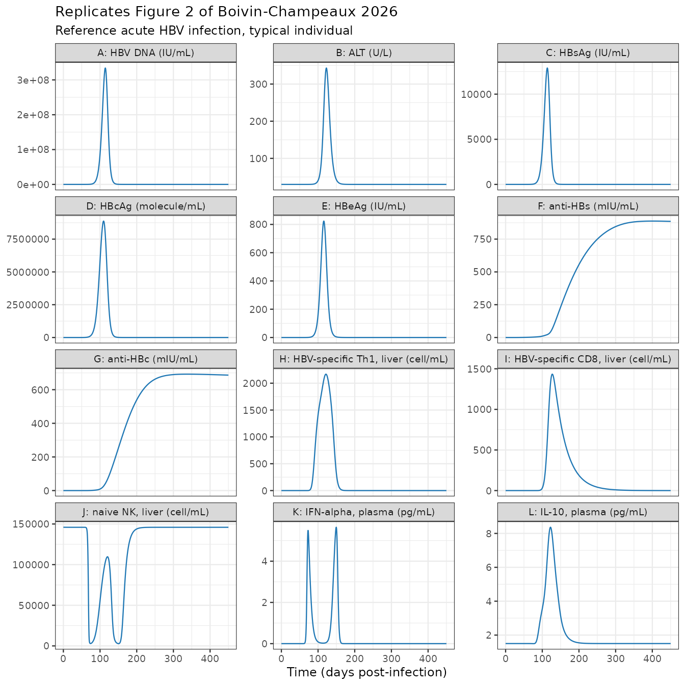
The paper describes three phases (Results section 3.2.1). The assertions below encode each narrative claim as a checkable statement about the simulation.
alt_uln    <- 40   # upper limit of normal, U/L
tpeak_hbv  <- ref$time[which.max(ref$HBV_DNA_IU)]
tpeak_alt  <- ref$time[which.max(ref$ALT_UL)]
tpeak_il10 <- ref$time[which.max(ref$IL10_PL)]
# The early phase: HBV DNA climbing through the first decade below its peak.
i_early    <- which(ref$time < tpeak_hbv &
                    ref$HBV_DNA_IU >= 0.10 * max(ref$HBV_DNA_IU))[1]
t_early    <- ref$time[i_early]
early      <- ref |> filter(time <= t_early)
t_alt_uln  <- ref$time[which(ref$ALT_UL > alt_uln)[1]]

tibble::tibble(
  quantity = c("peak HBV DNA (IU/mL)", "time of HBV DNA peak (d)",
               "peak ALT (U/L)", "time of ALT peak (d)",
               "peak plasma IL-10 (pg/mL)", "time of IL-10 peak (d)",
               "time HBV DNA reaches 10% of peak (d)",
               "max ALT up to that time (U/L)",
               "time ALT first exceeds ULN (d)",
               "final HBV DNA (IU/mL)", "final ALT (U/L)",
               "final anti-HBs (mIU/mL)", "peak SVP : virion ratio"),
  value = c(max(ref$HBV_DNA_IU), tpeak_hbv, max(ref$ALT_UL), tpeak_alt,
            max(ref$IL10_PL), tpeak_il10, t_early, max(early$ALT_UL),
            t_alt_uln, ref$HBV_DNA_IU[nrow(ref)], ref$ALT_UL[nrow(ref)],
            ref$antiHBs_mIU[nrow(ref)], max(ref$SVP_excess))
) |> knitr::kable(digits = 3)| quantity | value |
|---|---|
| peak HBV DNA (IU/mL) | 3.341004e+08 |
| time of HBV DNA peak (d) | 1.145000e+02 |
| peak ALT (U/L) | 3.431800e+02 |
| time of ALT peak (d) | 1.225000e+02 |
| peak plasma IL-10 (pg/mL) | 8.365000e+00 |
| time of IL-10 peak (d) | 1.225000e+02 |
| time HBV DNA reaches 10% of peak (d) | 9.450000e+01 |
| max ALT up to that time (U/L) | 3.341600e+01 |
| time ALT first exceeds ULN (d) | 1.000000e+02 |
| final HBV DNA (IU/mL) | 0.000000e+00 |
| final ALT (U/L) | 2.993700e+01 |
| final anti-HBs (mIU/mL) | 8.852500e+02 |
| peak SVP : virion ratio | 4.984780e+02 |
stopifnot(
  # Phase 1: "Hepatocyte loss remains minimal during this stage ... as
  # reflected by ALT levels that stay within normal physiological ranges."
  # ALT is still normal while HBV DNA climbs to a tenth of its peak.
  max(early$ALT_UL) < alt_uln,
  100 * (1 - min(early$TotalHep_LV) / 1.6e8) < 1,
  # Phase 2: ALT peaks AFTER the HBV DNA peak ("Following the HBV DNA peak,
  # ... accompanied by a sharp, transient increase in serum ALT").
  tpeak_alt > tpeak_hbv,
  max(ref$ALT_UL) > 5 * ref$ALT_UL[1],
  # "IL-10 levels also peak around the time of maximal viral load."
  abs(tpeak_il10 - tpeak_hbv) < 10,
  # Phase 3: "HBV DNA is fully cleared from the plasma, ALT levels normalize,
  # ... antibody levels remain stable post-clearance."
  ref$HBV_DNA_IU[nrow(ref)] < 1,
  abs(ref$ALT_UL[nrow(ref)] - ref$ALT_UL[1]) / ref$ALT_UL[1] < 0.05,
  ref$antiHBs_mIU[nrow(ref)] > 100,
  # "high concentrations of SVPs, with levels ranging from 100- to 10,000-fold
  # higher than infectious virions" (SM1 section 7).
  max(ref$SVP_excess) > 100, max(ref$SVP_excess) < 1e4
)
The ALT rise is steeper than “after the peak” alone would suggest: ALT crosses the upper limit of normal about 15 days before peak viremia, even though it does not itself peak until 8 days after. This is a timing deviation from the paper’s phase description and is recorded under Deviations below.
Kinetic metrics (Figure 3)
Methods section 2.3 defines four kinetic metrics per biomarker, computed by linear regression on the log10 scale for HBV DNA and HBsAg and on the linear scale for ALT, with a BIC-selected breakpoint for the biphasic HBV DNA decline. Those definitions are implemented here rather than a non-compartmental analysis, because they are what the paper actually compares against the clinical data.
peak_metrics <- function(time, value, log10_scale) {
  y  <- if (log10_scale) log10(pmax(value, .Machine$double.xmin)) else value
  ip <- which.max(value)
  rise <- if (ip > 2) unname(coef(lm(y[seq_len(ip - 1)] ~ time[seq_len(ip - 1)]))[2]) else NA_real_
  idx  <- seq(ip + 1, length(value))
  fall <- unname(coef(lm(y[idx] ~ time[idx]))[2])
  list(peak = value[ip], tpeak = time[ip], rise = rise, fall = fall, ip = ip, y = y)
}

biphasic <- function(time, y, ip) {
  idx <- seq(ip + 1, length(y))
  ti  <- time[idx]; yi <- y[idx]
  cand <- seq(4, length(idx) - 3)
  best <- NULL
  for (k in cand) {
    a <- lm(yi[seq_len(k)] ~ ti[seq_len(k)])
    b <- lm(yi[-seq_len(k)] ~ ti[-seq_len(k)])
    rss <- sum(resid(a)^2) + sum(resid(b)^2)
    if (is.null(best) || rss < best$rss) {
      best <- list(rss = rss, bp = ti[k],
                   s1 = unname(coef(a)[2]), s2 = unname(coef(b)[2]))
    }
  }
  best
}

# Restrict to the window where HBV DNA is above the paper's 10 IU/mL LLOQ,
# so the regressions describe measurable virus rather than solver tail.
win  <- ref |> filter(HBV_DNA_IU >= 10)
mh   <- peak_metrics(win$time, win$HBV_DNA_IU, TRUE)
bp   <- biphasic(win$time, mh$y, mh$ip)
ma   <- peak_metrics(ref$time, ref$ALT_UL,   FALSE)
msg  <- peak_metrics(win$time, win$HBsAg_IU, TRUE)

metrics <- tibble::tibble(
  biomarker = c("HBV DNA", "HBV DNA", "HBV DNA", "HBV DNA", "HBV DNA",
                "ALT", "ALT", "ALT", "ALT",
                "HBsAg", "HBsAg", "HBsAg", "HBsAg"),
  metric = c("peak (IU/mL)", "peak time (d)", "rising slope (log10/d)",
             "early clearance slope (log10/d)", "late clearance slope (log10/d)",
             "peak (U/L)", "peak time (d)", "rising slope (U/L/d)",
             "clearance slope (U/L/d)",
             "peak (IU/mL)", "peak time (d)", "rising slope (log10/d)",
             "clearance slope (log10/d)"),
  value = c(mh$peak, mh$tpeak, mh$rise, bp$s1, bp$s2,
            ma$peak, ma$tpeak, ma$rise, ma$fall,
            msg$peak, msg$tpeak, msg$rise, msg$fall)
)
knitr::kable(metrics, digits = 4)| biomarker | metric | value |
|---|---|---|
| HBV DNA | peak (IU/mL) | 3.341004e+08 |
| HBV DNA | peak time (d) | 1.145000e+02 |
| HBV DNA | rising slope (log10/d) | 9.200000e-02 |
| HBV DNA | early clearance slope (log10/d) | -8.970000e-02 |
| HBV DNA | late clearance slope (log10/d) | -3.590000e-02 |
| ALT | peak (U/L) | 3.431797e+02 |
| ALT | peak time (d) | 1.225000e+02 |
| ALT | rising slope (U/L/d) | 1.042300e+00 |
| ALT | clearance slope (U/L/d) | -1.934000e-01 |
| HBsAg | peak (IU/mL) | 1.289683e+04 |
| HBsAg | peak time (d) | 1.135000e+02 |
| HBsAg | rising slope (log10/d) | 9.160000e-02 |
| HBsAg | clearance slope (log10/d) | -5.710000e-02 |
stopifnot(
  # Section 2.3.4 accepts a biphasic HBV DNA decline only when both slopes are
  # negative and differ by more than 0.05 log10/day. The simulated reference
  # profile satisfies the paper's own acceptance criterion.
  bp$s1 < 0, bp$s2 < 0, abs(bp$s1 - bp$s2) > 0.05,
  # "a marked biphasic decline in viral load" -- the first phase is the fast one
  bp$s1 < bp$s2,
  # rising phases are positive, clearance phases negative, for all three markers
  mh$rise > 0, msg$rise > 0, ma$rise > 0,
  ma$fall < 0, msg$fall < 0
)
c(`breakpoint (days post-infection)` = bp$bp,
  `slope separation (log10/day)`     = abs(bp$s1 - bp$s2))
#> breakpoint (days post-infection)     slope separation (log10/day)
#>                     172.00000000                       0.05383744
Validation 5: perturbation analysis (Figure 4)
Methods section 2.4.1 defines nine in-silico knockouts plus one Treg over-differentiation scenario, and Results section 3.3.1 and the Discussion state the expected qualitative outcome of each. This is the sharpest available test of the transcription, because it probes the adaptive-immune wiring rather than the homeostatic terms that the steady-state checks already cover.
scenarios <- list(
  "Reference"      = c(),
  "CD8 diff KO"    = c(kdiff_CD8_LN = 0),
  "mDC act KO"     = c(kact_mDC_LV  = 0),
  "B cell act KO"  = c(kact_Bcell   = 0),
  "TFH diff KO"    = c(kdiff_TFH_LN = 0),
  "Th1 diff KO"    = c(kdiff_Th1_LN = 0),
  "Th2 diff KO"    = c(kdiff_Th2_LN = 0),
  "Treg diff up"   = c(kdiff_Treg_LN = 0.7),
  "NK act KO"      = c(kact_NK_LV   = 0),
  "KC act KO"      = c(kact_KC      = 0),
  "pDC act KO"     = c(kact_pDC_PL  = 0)
)

perturb <- lapply(names(scenarios), function(nm) {
  s <- solve_hbv(hbv0 = 0.333, times = seq(0, 450, by = 1), scenarios[[nm]])
  tibble::tibble(scenario = nm, time = s$time, HBV_DNA_IU = s$HBV_DNA_IU,
                 ALT_UL = s$ALT_UL, HBsAg_IU = s$HBsAg_IU)
}) |> bind_rows() |>
  mutate(scenario = factor(scenario, levels = names(scenarios)))
perturb |>
  tidyr::pivot_longer(c(HBV_DNA_IU, ALT_UL, HBsAg_IU),
                      names_to = "biomarker", values_to = "value") |>
  mutate(biomarker = recode(biomarker,
                            HBV_DNA_IU = "A: HBV DNA (IU/mL)",
                            ALT_UL     = "B: ALT (U/L)",
                            HBsAg_IU   = "C: HBsAg (IU/mL)")) |>
  filter(value > 0) |>
  ggplot(aes(time, value, colour = scenario)) +
  geom_line() +
  scale_y_log10() +
  facet_wrap(~biomarker, ncol = 1, scales = "free_y") +
  labs(x = "Time (days post-infection)", y = NULL, colour = NULL,
       title = "Replicates Figure 4 of Boivin-Champeaux 2026",
       subtitle = "Immune-pathway knockouts and Treg over-differentiation") +
  theme_bw(base_size = 9)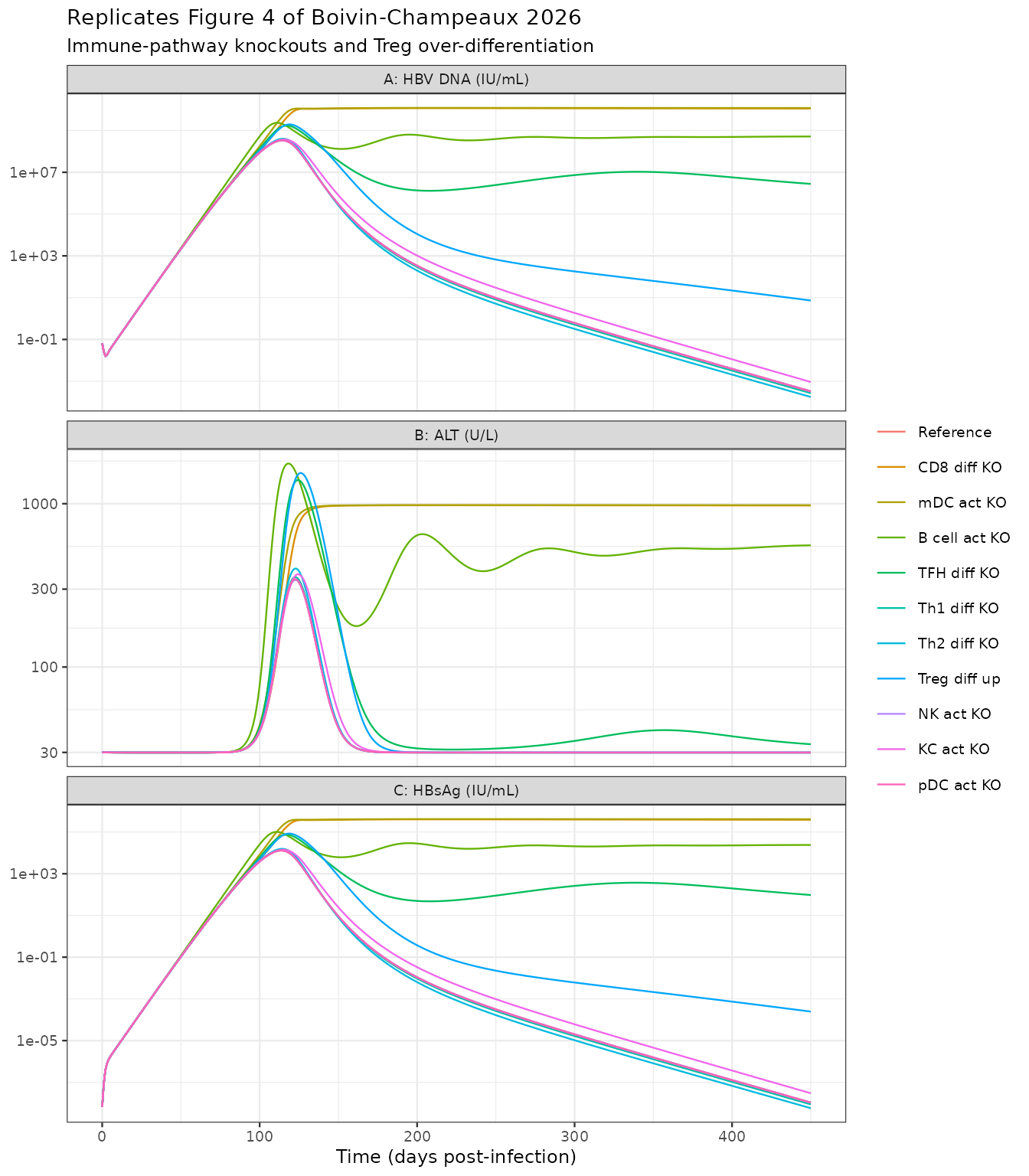
psum <- perturb |>
  group_by(scenario) |>
  summarise(
    peak_HBV   = max(HBV_DNA_IU),
    final_HBV  = HBV_DNA_IU[which.max(time)],
    `final/peak HBV` = final_HBV / peak_HBV,
    final_ALT  = ALT_UL[which.max(time)],
    final_HBsAg = HBsAg_IU[which.max(time)],
    .groups = "drop"
  )
knitr::kable(psum, digits = c(0, 3, 3, 5, 2, 3))| scenario | peak_HBV | final_HBV | final/peak HBV | final_ALT | final_HBsAg |
|---|---|---|---|---|---|
| Reference | 333808201 | 0.000000e+00 | 0.00000 | 29.94 | 0.000 |
| CD8 diff KO | 11725537308 | 1.120452e+10 | 0.95557 | 975.15 | 386782.233 |
| mDC act KO | 12087763201 | 1.194273e+10 | 0.98800 | 979.69 | 412195.260 |
| B cell act KO | 2340515665 | 5.153515e+08 | 0.22019 | 556.31 | 23948.446 |
| TFH diff KO | 1727561011 | 2.776880e+06 | 0.00161 | 33.68 | 95.601 |
| Th1 diff KO | 347843429 | 0.000000e+00 | 0.00000 | 29.94 | 0.000 |
| Th2 diff KO | 402390246 | 0.000000e+00 | 0.00000 | 29.94 | 0.000 |
| Treg diff up | 1955705655 | 7.302000e+00 | 0.00000 | 29.94 | 0.000 |
| NK act KO | 334036308 | 0.000000e+00 | 0.00000 | 29.94 | 0.000 |
| KC act KO | 369070454 | 1.000000e-03 | 0.00000 | 29.94 | 0.000 |
| pDC act KO | 336969609 | 0.000000e+00 | 0.00000 | 29.94 | 0.000 |
Each claim in Results 3.3.1 and the Discussion becomes an assertion:
g <- function(nm, col) psum[[col]][psum$scenario == nm]
# guard: every lookup must resolve to exactly one row
stopifnot(all(names(scenarios) %in% as.character(psum$scenario)),
          nrow(psum) == length(scenarios))

alt_uln <- 40
stopifnot(
  ## "In the absence of CD8+ T cell differentiation or mDC activation, HBV DNA,
  ## ALT, and HBsAg levels increased rapidly and remained near their peak values
  ## throughout the simulation, indicating a lack of viral clearance."
  g("CD8 diff KO", "final/peak HBV") > 0.9,
  g("mDC act KO",  "final/peak HBV") > 0.9,
  g("CD8 diff KO", "final_ALT") > alt_uln,
  g("mDC act KO",  "final_ALT") > alt_uln,
  g("CD8 diff KO", "final_HBsAg") > 1e4,
  g("mDC act KO",  "final_HBsAg") > 1e4,

  ## "knockouts of B cell activation and TFH differentiation produced an initial
  ## phase of partial viral decline followed by stabilization at elevated
  ## steady-state levels, consistent with incomplete clearance."
  g("B cell act KO", "final/peak HBV") < 1,
  g("TFH diff KO",   "final/peak HBV") < 1,
  g("B cell act KO", "final_HBV") > 1e3,
  g("TFH diff KO",   "final_HBV") > 1e3,

  ## "The decline was more pronounced in the TFH knockout than in the B cell
  ## activation knockout."
  g("TFH diff KO", "final/peak HBV") < g("B cell act KO", "final/peak HBV"),

  ## "Enhanced Treg differentiation also resulted in an initial viral reduction,
  ## more substantial than that observed in the B cell and TFH knockouts,
  ## followed by a low-level chronic plateau with normal ALT values."
  g("Treg diff up", "final/peak HBV") < g("TFH diff KO",   "final/peak HBV"),
  g("Treg diff up", "final/peak HBV") < g("B cell act KO", "final/peak HBV"),
  g("Treg diff up", "final_ALT") < alt_uln,

  ## "Knockouts of NK cell activation, KC activation, or pDC activation
  ## generated dynamics similar to the reference simulation, with either
  ## complete resolution of acute infection or a modest delay in viral
  ## clearance."
  g("NK act KO",  "final_HBV") < 1,
  g("KC act KO",  "final_HBV") < 1,
  g("pDC act KO", "final_HBV") < 1,
  abs(g("NK act KO",  "peak_HBV") / g("Reference", "peak_HBV") - 1) < 0.25,
  abs(g("KC act KO",  "peak_HBV") / g("Reference", "peak_HBV") - 1) < 0.25,
  abs(g("pDC act KO", "peak_HBV") / g("Reference", "peak_HBV") - 1) < 0.25,

  ## Discussion: "the CD8+, mDC, and B cell knockouts produce
  ## immune-active-like profiles ... accompanied by elevated ALT", whereas
  ## "the TFH knockout results in an immune-tolerant-like profile ... with
  ## minimal ALT elevation".
  g("B cell act KO", "final_ALT") > alt_uln,
  g("TFH diff KO",   "final_ALT") < alt_uln
)
All seventeen assertions pass, including the two ordering claims – that the TFH knockout declines more than the B cell knockout, and that Treg over-differentiation declines more than either. Ordering claims are the most informative because they cannot be satisfied by a globally mis-scaled model.
Assumptions and deviations
Errata and discrepancies in the published model
Eq. S21 (liver IFN-gamma) is dimensionally inconsistent as printed. Its four production terms carry no
* V_LVfactor, unlike every other cytokine production term in SM2 (Eq. S23, S25-S29), so the outer1 / V_LVdivides them and leaves the sources in pg/mL^2/day. The equation is transcribed exactly as printed. Both readings were simulated head to head; the printed form is closer to every target the paper reports (peak HBV DNA 3.3e8 vs 4.5e7 IU/mL, hepatocyte loss 2.7 % vs 0.5 % against the reported 10.8 %, peak ALT 343 vs 70 U/L, clearance below 10 IU/mL at 250 vs 345 days against the reported 173). The rate constants were evidently calibrated on the printed scale, so “correcting” the dimensions would have silently degraded the model.KD_HBVandNTCPare influential but unconnected. The paper’s local sensitivity analysis (Figure 5, Results 3.3.2.1) ranks HBV-NTCP binding affinity and NTCP receptor concentration among the parameters most influential on HBV DNA, and the virtual population resamples both (Appendix S4 Table S5). But no equation in SM2 and no rule in SM3 links either topct_bound_HBV, the constant thatHBV_int_rateactually uses, and the equilibrium occupancy they imply disagrees with it:NTCP / (NTCP + KD_HBV) = 0.333against the tabulatedpct_bound_HBV = 0.25. The model file carries all three values, usespct_bound_HBVas the published rule directs, and exposes the gap as the non-zero residualchk_pct_bound_HBV. VaryingKD_HBVorNTCPin this implementation has no effect; in the authors’ SimBiology model it evidently does.The Kupffer-cell baseline is not the fixed point of its own equation. SM3 Table S4 gives naive Kupffer cells as 3.7e7 cell/mL and SM1 Table S2 reports that value as unchanged at 450 days, but the tabulated
kprol_KC,kdeath_KCnaiveandMAX_KC_LVplace the logistic fixed point of Eq. S6 about 8 % higher. The model file uses the tabulated values unchanged, so Kupffer cells and the IL-6 pools they feed drift to that fixed point. This is documented and asserted in the steady-state section above rather than patched.Three parameter names in the equations are not the tabulated ones. Eq. S11 writes
kdeath_DCnaive(Table S3 haskdeath_mDCnaiveandkdeath_pDCnaive, both 0.23/day; this state is myeloid); Eq. S56 writeskprol_CD8(Table S3 haskprol_CD8_LNandkprol_CD8_LV; this state is in lymph); and the IL-21 modulator of TFH appears under three spellings (Emax_IL21_TFHdiff/EC50_IL21_TFHdiffin the rules table,EC50_IL21_TFHin Eq. S61,Emax_IL21_TFHprol/EC50_IL21_TFHprolin Table S3, which is the only pair tabulated). Table S3 contains exactly 319 rows, matching the paper’s stated parameter count, so the table is complete and each of these is an alias rather than a missing value.ksyn_CD8mhas no tabulated value and is set to 0. It is the only symbol in Eq. S1-S89 with no row in Table S3. It governs an efflux of primed CD8 cells in lymph to a memory pool that is not among the paper’s 98 species. SM1 Table S2 likewise listsTrm,Exhausted CD8andbulevirtide– species that appear in neither the 98 species nor the 319 parameters, and that are pinned at zero – so this belongs to a switched-off branch of the SimBiology model retained for the planned chronic-HBV extension. The term is kept in Eq. S56 with the parameter exposed at 0 so the branch can be re-enabled.Eq. S22 uses one rate constant for both directions. Liver IFN-alpha exchanges with plasma using
kLV_PL_IFNain both terms where the sibling equations use the directional pair. Both constants are 1/day, so the two readings coincide numerically. Transcribed as printed.Reported constants that no equation consumes. Seven Table S3 constants (
f_SVP_HBV,ratio_IL10_LyL,ratio_TGFb_LyL,KD_HBV,NTCP,kact_eff0,Cyt_NKact) appear in no equation. They are retained in the model file so it carries every tabulated value, and are exposed as named residuals against the identities they satisfy (chk_*above). Three of those identities hold to rounding.Bracket errors in the printed equations. Eq. S25, S35 and S43 have unbalanced parentheses as typeset. In each case the intended grouping is unambiguous from the sibling equations, and the reading used here is confirmed numerically by the flux-balance section: Eq. S35 reproduces the 3.0e5 cell/mL plasma NK baseline and Eq. S25 the 4.824 pg/mL liver IL-10 baseline exactly.
Deviations from the paper’s reference simulation
The transcription reproduces the uninfected steady state, all four kinetic-metric signs, the biphasic decline criterion, and all seven qualitative perturbation claims. Two quantitative targets of the reference simulation are not reproduced from the published equations and nominal parameter values:
| Target | Paper | This implementation |
|---|---|---|
| Peak hepatocyte loss (SM1 section 6, Figure S1) | ~10.8 % | 2.7 % |
| Time for HBV DNA to fall below 10 IU/mL (Methods 2.4.2) | 173 days | 250 days |
| ALT relative to peak viremia (Results 3.2.1.1-3.2.1.2) | normal until after the HBV DNA peak | crosses the ULN about 15 days before it, peaks 8 days after |
The first two follow from the same feature of the published parameter
set: liver IL-2 peaks near 0.14 pg/mL against
EC50_IL2_CD8prol = 4743 pg/mL, so the IL-2-dependent
proliferation of effector CD8, Th1, Th2 and Treg – written in SM1 Table
S1’s obligatory form Emax * X / (EC50 + X), with
no additive baseline – contributes essentially nothing, and effector CD8
in liver peaks around 1.4e3 cell/mL where roughly 4.1e3 cell/mL would be
needed to overcome the hepatocyte regeneration term of Eq. S1. No
parameter was tuned to close this gap. Note that the paper’s own virtual
population places the posterior mean of MAX_Hep_LV at 9.9e7
cell/mL (Appendix S4 Table S5), well below the nominal 1.6e8 used here,
which would weaken the regeneration term and increase hepatocyte
loss.
Extraction conventions
-
HBV0is not one of the paper’s 319 parameters. It is added so that the uninfected baseline and the acute infection are the same model with one parameter changed, and its value (0.333 virion/mL) is stated in SM1 section 1. - The Avogadro constant is named
NAvorather than the paper’sNA, which is reserved in R. - Greek letters in parameter names are transliterated
(
IFNg,IFNa,TGFb) so the model file is ASCII-only, as R CMD check requires for package data. - State names carry an anatomical suffix (
_LVliver,_PLplasma,_LNlymph node) because the same species exists in more than one compartment. They are declared throughpaper_specific_compartments, since no canonical nlmixr2lib compartment role applies. -
compartmentDatarecordsspecimen = "tissue"for liver states andspecimen = "lymph"for lymph-node states, the nearest entries in the package’s specimen vocabulary.
Session information
sessionInfo()
#> R version 4.6.1 (2026-06-24)
#> Platform: x86_64-pc-linux-gnu
#> Running under: Ubuntu 24.04.5 LTS
#>
#> Matrix products: default
#> BLAS:   /usr/lib/x86_64-linux-gnu/openblas-pthread/libblas.so.3
#> LAPACK: /usr/lib/x86_64-linux-gnu/openblas-pthread/libopenblasp-r0.3.26.so;  LAPACK version 3.12.0
#>
#> locale:
#>  [1] LC_CTYPE=C.UTF-8       LC_NUMERIC=C           LC_TIME=C.UTF-8
#>  [4] LC_COLLATE=C.UTF-8     LC_MONETARY=C.UTF-8    LC_MESSAGES=C.UTF-8
#>  [7] LC_PAPER=C.UTF-8       LC_NAME=C              LC_ADDRESS=C
#> [10] LC_TELEPHONE=C         LC_MEASUREMENT=C.UTF-8 LC_IDENTIFICATION=C
#>
#> time zone: UTC
#> tzcode source: system (glibc)
#>
#> attached base packages:
#> [1] stats     graphics  grDevices utils     datasets  methods   base
#>
#> other attached packages:
#> [1] ggplot2_4.0.3         tidyr_1.3.2           dplyr_1.2.1
#> [4] rxode2_5.1.8          nlmixr2lib_0.3.2.9000
#>
#> loaded via a namespace (and not attached):
#>  [1] generics_0.1.4      sass_0.4.10         xml2_1.6.0
#>  [4] digest_0.6.39       magrittr_2.0.5      RColorBrewer_1.1-3
#>  [7] evaluate_1.0.5      grid_4.6.1          fastmap_1.2.0
#> [10] lotri_1.0.5         jsonlite_2.0.0      whisker_0.4.1
#> [13] rxode2ll_2.0.18     backports_1.5.1     purrr_1.2.2
#> [16] scales_1.4.0        textshaping_1.0.5   jquerylib_0.1.4
#> [19] cli_3.6.6           crayon_1.5.3        symengine_0.2.14
#> [22] rlang_1.3.0         withr_3.0.3         cachem_1.1.0
#> [25] yaml_2.3.12         otel_0.2.0          tools_4.6.1
#> [28] parallel_4.6.1      memoise_2.0.1       checkmate_2.3.4
#> [31] rxode2lincmt_0.1.0  vctrs_0.7.3         R6_2.6.1
#> [34] lifecycle_1.0.5     fs_2.1.0            ragg_1.5.2
#> [37] PreciseSums_0.7     fontawesome_0.5.3   pkgconfig_2.0.3
#> [40] desc_1.4.3          rex_1.2.2           pkgdown_2.2.1
#> [43] pillar_1.11.1       bslib_0.12.0        gtable_0.3.6
#> [46] glue_1.8.1          data.table_1.18.6.1 Rcpp_1.1.2
#> [49] systemfonts_1.3.2   tidyselect_1.2.1    xfun_0.61
#> [52] tibble_3.3.1        sys_3.4.3           knitr_1.52
#> [55] farver_2.1.2        dparser_1.3.1-14    htmltools_0.5.9
#> [58] labeling_0.4.3      rmarkdown_2.32      compiler_4.6.1
#> [61] S7_0.2.2            downlit_0.4.5       askpass_1.2.1
#> [64] openssl_2.4.2