Rivaroxaban (Willmann 2018)
Source:vignettes/articles/Willmann_2018_rivaroxaban.Rmd
Willmann_2018_rivaroxaban.RmdModel and source
- Citation: Willmann S, Thelen K, Kubitza D, Lensing AWA, Frede M, Coboeken K, Stampfuss J, Burghaus R, Mueck W, Lippert J. Pharmacokinetics of rivaroxaban in children using physiologically based and population pharmacokinetic modelling: an EINSTEIN-Jr phase I study. Thrombosis Journal. 2018;16:32.
- Article: https://doi.org/10.1186/s12959-018-0185-1
- Trial registration: ClinicalTrials.gov NCT01145859 (EINSTEIN-Jr phase I).
Population
The EINSTEIN-Jr phase I single-dose study (Willmann 2018) enrolled 59 children aged 0.5-18 years across 18 sites in 7 countries (Australia, Austria, Canada, France, Israel, Italy, United States) between November 2010 and July 2015. All participants had completed treatment for venous thromboembolism (VTE). Subjects received a single body-weight-adjusted oral dose of rivaroxaban targeting adult exposure of either rivaroxaban 10 mg or 20 mg, in one of four age strata (0.5-<2, 2-<6, 6-<12, 12-<18 years). Children aged >=12 years received the tablet formulation; children aged 6-<12 years received tablet or oral suspension (undiluted or diluted) at the discretion of the investigator; children aged <6 years received the oral suspension only. The 59 children contributed 206 plasma concentrations, 7 of which were below the LLOQ (0.500 ug/L) and excluded; the remaining 199 measurements were used in the popPK fit (Willmann 2018 Results paragraph 1; detailed baseline demographics are reported in the accompanying clinical study publication, reference 18 of Willmann 2018).
mod_meta <- readModelDb("Willmann_2018_rivaroxaban")
mod_meta()$population
#> $species
#> [1] "human"
#>
#> $n_subjects
#> [1] 59
#>
#> $n_studies
#> [1] 1
#>
#> $age_range
#> [1] "0.5-18 years (four cohorts: 0.5-<2, 2-<6, 6-<12, 12-<18 years)"
#>
#> $weight_range
#> [1] "approximately 5-80 kg across the 0.5-18-year cohorts (the paper reports detailed weight ranges in the accompanying study report, reference 18)"
#>
#> $sex_female_pct
#> [1] NA
#>
#> $disease_state
#> [1] "Children who had completed treatment for venous thromboembolism (VTE); EINSTEIN-Jr phase I single-dose pharmacokinetic study."
#>
#> $dose_range
#> [1] "Body-weight-adjusted single oral doses targeting adult exposure of either rivaroxaban 10 mg or 20 mg, delivered as tablet (children >=6 years at investigator discretion; required for children >=12 years), undiluted oral suspension, or diluted oral suspension (required for children <6 years)."
#>
#> $regions
#> [1] "18 sites in 7 countries: Australia, Austria, Canada, France, Israel, Italy, United States."
#>
#> $n_observations
#> [1] "206 plasma concentrations from 59 children; 7 below LLOQ (0.500 ug/L) excluded, leaving 199 for the popPK fit."
#>
#> $trial_id
#> [1] "NCT01145859 (EINSTEIN-Jr phase I)."
#>
#> $notes
#> [1] "Demographic and dosing summary from Willmann 2018 Methods (Participants and study design) and Results (paragraph 1); detailed baseline demographics are reported in the accompanying clinical study publication (reference 18 of Willmann 2018, Monagle et al.). Sampling windows were age-dependent: 90 min-5 h and 20-24 h in children aged 0.5-2 years, with an additional 8-12 h sample in 2-6 year-olds; children >=6 years contributed up to four samples within 24 h post-dose."
Source trace
The per-parameter origin is recorded as an in-file comment next to
each ini() entry in
inst/modeldb/specificDrugs/Willmann_2018_rivaroxaban.R. The
table below collects them in one place for review. All values come from
Willmann 2018 Table 1 (“Population estimates for the first pediatric
PopPK model of rivaroxaban”).
| Equation / parameter | Value | Source location |
|---|---|---|
lka (typical ka, tablet / diluted suspension) |
log(0.717) 1/h | Table 1, row “ka for tablet and diluted suspension” |
e_undilsusp_ka (log-shift on ka, undiluted susp.) |
log(0.208/0.717) | Table 1, row “ka for undiluted suspension” (0.208 1/h) |
lcl (typical CL/F at 70 kg) |
log(7.26) L/h | Table 1, row “CL” |
lvc (typical V/F at 70 kg) |
log(50.9) L | Table 1, row “V” |
lq (typical Q/F) |
log(0.928) L/h | Table 1, row “Q” |
lvp (typical Vp/F) |
log(13.5) L | Table 1, row “Vp” |
allo_cl (allometric exponent on CL) |
0.323 (estimated) | Table 1, row “Exponent for CL scaling” |
allo_vc (allometric exponent on V) |
1.0 (fixed) | Table 1, row “Exponent for V scaling”; Results paragraph 4 |
lfdepot (F1 for 20 mg-eq vs 10 mg-eq) |
log(0.648) | Table 1, row “F1” |
etalka (IIV variance) |
log(1 + 0.397^2) | Table 1, row “ka …” IIV CV 39.7% |
etalcl (IIV variance) |
log(1 + 0.262^2) | Table 1, row “CL” IIV CV 26.2% |
propSd (proportional residual error SD) |
0.466 | Table 1, row “Residual error (%)” |
| Structural: linear two-compartment, first-order abs | n/a | Methods, “Development of a first PopPK model in children” paragraph 2 |
| Allometric scaling on CL and V relative to 70 kg | n/a | Methods, “Development of a first PopPK model in children” paragraph 3 |
| No allometric scaling on Q or Vp | n/a | Results, “Parameters of the first PopPK model” paragraph 1 |
| Proportional residual error | n/a | Results, “Parameters of the first PopPK model” paragraph 1 |
Virtual cohort
Original observed data are not publicly available. The figures below
use virtual populations whose covariate distributions approximate the
Willmann 2018 EINSTEIN-Jr phase I demographics: four age cohorts (0.5-2,
2-6, 6-12, 12-18 years) crossed with two dose levels (10 mg-equivalent,
20 mg-equivalent). Cohort weights are drawn from age-appropriate normal
distributions; the formulation per cohort follows the paper’s
predominant assignment scheme. The body-weight-adjusted dose is computed
as nominal_dose * (WT / 70)^0.323 so that, under the
model’s allometric scaling on CL (estimated exponent 0.323), the
simulated AUC matches the 70 kg adult-equivalent exposure target (this
is the dosing-design intent of the EINSTEIN-Jr phase I study; the
paper’s actual dose-by-weight table is reported in the accompanying
clinical publication, reference 18 of Willmann 2018).
Cohort size is 100 children per (age x dose) cell, well under the 200/arm cap.
set.seed(42)

# Age-cohort summary: representative weight distribution and dominant
# formulation per Willmann 2018 Participants and Study Design.
cohorts_meta <- tibble::tribble(
  ~age_group, ~wt_mean, ~wt_sd, ~form_undil_susp, ~formulation_label,
  "0.5-2y",      10,      1.5,                0L, "Diluted suspension",
  "2-6y",        17,      3.0,                0L, "Diluted suspension",
  "6-12y",       30,      6.0,                0L, "Tablet (or diluted suspension)",
  "12-18y",      55,     10.0,                0L, "Tablet"
)

doses_meta <- tibble::tibble(
  dose_group = c("10 mg-eq", "20 mg-eq"),
  nominal_mg = c(10, 20),
  DOSE_HIGH_RIV = c(0L, 1L)
)

design_grid <- tidyr::crossing(cohorts_meta, doses_meta) |>
  dplyr::mutate(treatment = paste(age_group, dose_group, sep = " / "))

n_per_cell <- 100L
obs_times  <- c(0, 0.25, 0.5, 0.75, 1, 1.5, 2, 3, 4, 6, 8, 12, 16, 20, 24)

make_cohort <- function(meta_row, id_offset) {
  n  <- n_per_cell
  wt <- pmax(2.5,
             stats::rnorm(n, mean = meta_row$wt_mean, sd = meta_row$wt_sd))
  subj <- tibble::tibble(
    id            = id_offset + seq_len(n),
    WT            = wt,
    FORM_UNDIL_SUSP = meta_row$form_undil_susp,
    DOSE_HIGH_RIV = meta_row$DOSE_HIGH_RIV,
    treatment     = meta_row$treatment,
    age_group     = meta_row$age_group,
    dose_group    = meta_row$dose_group,
    formulation_label = meta_row$formulation_label,
    nominal_mg    = meta_row$nominal_mg
  )
  # Body-weight-adjusted dose targeting adult-equivalent exposure under the
  # estimated allometric CL exponent 0.323.
  dose_rows <- subj |>
    dplyr::mutate(time = 0,
                  evid = 1L,
                  amt  = nominal_mg * (WT / 70)^0.323,
                  cmt  = "depot")
  obs_rows <- subj |>
    tidyr::crossing(time = obs_times) |>
    dplyr::mutate(evid = 0L,
                  amt  = NA_real_,
                  cmt  = "central")
  dplyr::bind_rows(dose_rows, obs_rows) |>
    dplyr::arrange(id, time, dplyr::desc(evid))
}

events <- purrr::reduce(
  seq_len(nrow(design_grid)),
  function(acc, i) {
    dplyr::bind_rows(acc,
                     make_cohort(design_grid[i, ],
                                 id_offset = (i - 1L) * n_per_cell))
  },
  .init = tibble::tibble()
)

stopifnot(!anyDuplicated(unique(events[, c("id", "time", "evid")])))
events_n <- length(unique(events$id))
cat("Total simulated subjects:", events_n, "across",
    nrow(design_grid), "(age x dose) cells.\n")
#> Total simulated subjects: 800 across 8 (age x dose) cells.
Simulation
mod <- readModelDb("Willmann_2018_rivaroxaban")

sim <- rxode2::rxSolve(
  mod,
  events = events,
  keep = c("WT", "FORM_UNDIL_SUSP", "DOSE_HIGH_RIV",
           "treatment", "age_group", "dose_group",
           "formulation_label", "nominal_mg")
) |>
  as.data.frame() |>
  dplyr::as_tibble()
#> ℹ parameter labels from comments will be replaced by 'label()'
For deterministic typical-value replication (no between-subject variability):
mod_typical <- mod |> rxode2::zeroRe()
#> ℹ parameter labels from comments will be replaced by 'label()'
sim_typical <- rxode2::rxSolve(
  mod_typical,
  events = events,
  keep = c("WT", "FORM_UNDIL_SUSP", "DOSE_HIGH_RIV",
           "treatment", "age_group", "dose_group",
           "formulation_label", "nominal_mg")
) |>
  as.data.frame() |>
  dplyr::as_tibble()
#> ℹ omega/sigma items treated as zero: 'etalka', 'etalcl'
#> Warning: multi-subject simulation without without 'omega'
Replicate Figure 3 -plasma concentration vs time by age x dose cell
Willmann 2018 Figure 3 panels (a)-(h) plot observed plasma concentrations vs time for each (age x dose) combination. Each panel here is a simulation-based visual predictive check (median + 5/95 percentile ribbon) at the same age x dose stratification. The model’s two-compartment structure, formulation- dependent absorption, dose-dependent F1, and weight-allometric CL / Vc are all exercised.
sim_summary <- sim |>
  dplyr::filter(time > 0) |>
  dplyr::group_by(age_group, dose_group, time) |>
  dplyr::summarise(
    Q05 = quantile(Cc, 0.05, na.rm = TRUE),
    Q50 = quantile(Cc, 0.50, na.rm = TRUE),
    Q95 = quantile(Cc, 0.95, na.rm = TRUE),
    .groups = "drop"
  ) |>
  dplyr::mutate(
    age_group  = factor(age_group,
                        levels = c("0.5-2y", "2-6y", "6-12y", "12-18y")),
    dose_group = factor(dose_group, levels = c("10 mg-eq", "20 mg-eq"))
  )

ggplot(sim_summary, aes(time, Q50)) +
  geom_ribbon(aes(ymin = Q05, ymax = Q95), alpha = 0.25) +
  geom_line() +
  facet_grid(dose_group ~ age_group) +
  scale_y_log10() +
  labs(x = "Time post dose (h)", y = "Rivaroxaban Cc (ug/L)",
       title = "Figure 3 -simulated VPC by age x dose cell",
       caption = "Replicates Figure 3 panels of Willmann 2018; median + 5/95 percentile ribbon.")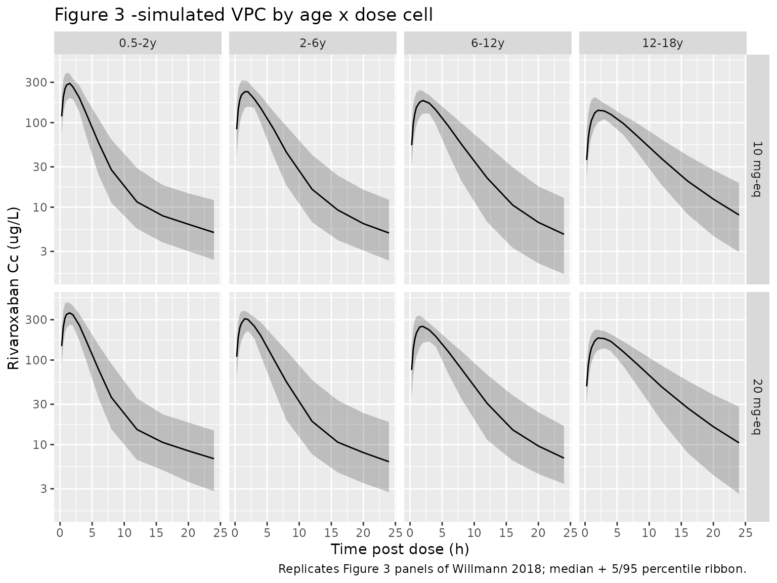
Replicate the formulation effect on absorption
Willmann 2018 estimated ka ~3.4-fold slower for the
undiluted oral suspension (0.208 1/h) than for the tablet or diluted
oral suspension (0.717 1/h). This side-by-side typical-value simulation
in a representative 6-12 y child holds all other covariates
constant.
formulation_demo <- tibble::tribble(
  ~id, ~time, ~evid, ~amt, ~cmt,      ~WT, ~FORM_UNDIL_SUSP, ~DOSE_HIGH_RIV,
   1L,  0,    1L,    10,   "depot",    30,    0L,               0L,
   2L,  0,    1L,    10,   "depot",    30,    1L,               0L
) |>
  dplyr::bind_rows(
    tidyr::crossing(id = c(1L, 2L), time = obs_times) |>
      dplyr::mutate(evid = 0L, amt = NA_real_, cmt = "central",
                    WT = 30,
                    FORM_UNDIL_SUSP = ifelse(id == 1L, 0L, 1L),
                    DOSE_HIGH_RIV = 0L)
  ) |>
  dplyr::arrange(id, time, dplyr::desc(evid))

sim_form <- rxode2::rxSolve(
  rxode2::zeroRe(mod),
  events = formulation_demo,
  keep = c("FORM_UNDIL_SUSP", "WT")
) |>
  as.data.frame() |>
  dplyr::as_tibble() |>
  dplyr::filter(time > 0) |>
  dplyr::mutate(
    formulation = ifelse(FORM_UNDIL_SUSP == 1L,
                         "Undiluted suspension (ka = 0.208 1/h)",
                         "Tablet or diluted suspension (ka = 0.717 1/h)")
  )
#> ℹ parameter labels from comments will be replaced by 'label()'
#> ℹ omega/sigma items treated as zero: 'etalka', 'etalcl'
#> Warning: multi-subject simulation without without 'omega'

ggplot(sim_form, aes(time, Cc, colour = formulation)) +
  geom_line(linewidth = 1) +
  scale_colour_manual(values = c("steelblue4", "darkorange3")) +
  labs(x = "Time post dose (h)", y = "Rivaroxaban Cc (ug/L)",
       title = "Formulation effect on absorption (typical value)",
       caption = "30 kg child, 10 mg-equivalent dose; deterministic typical-value simulation.",
       colour = NULL) +
  theme(legend.position = "bottom")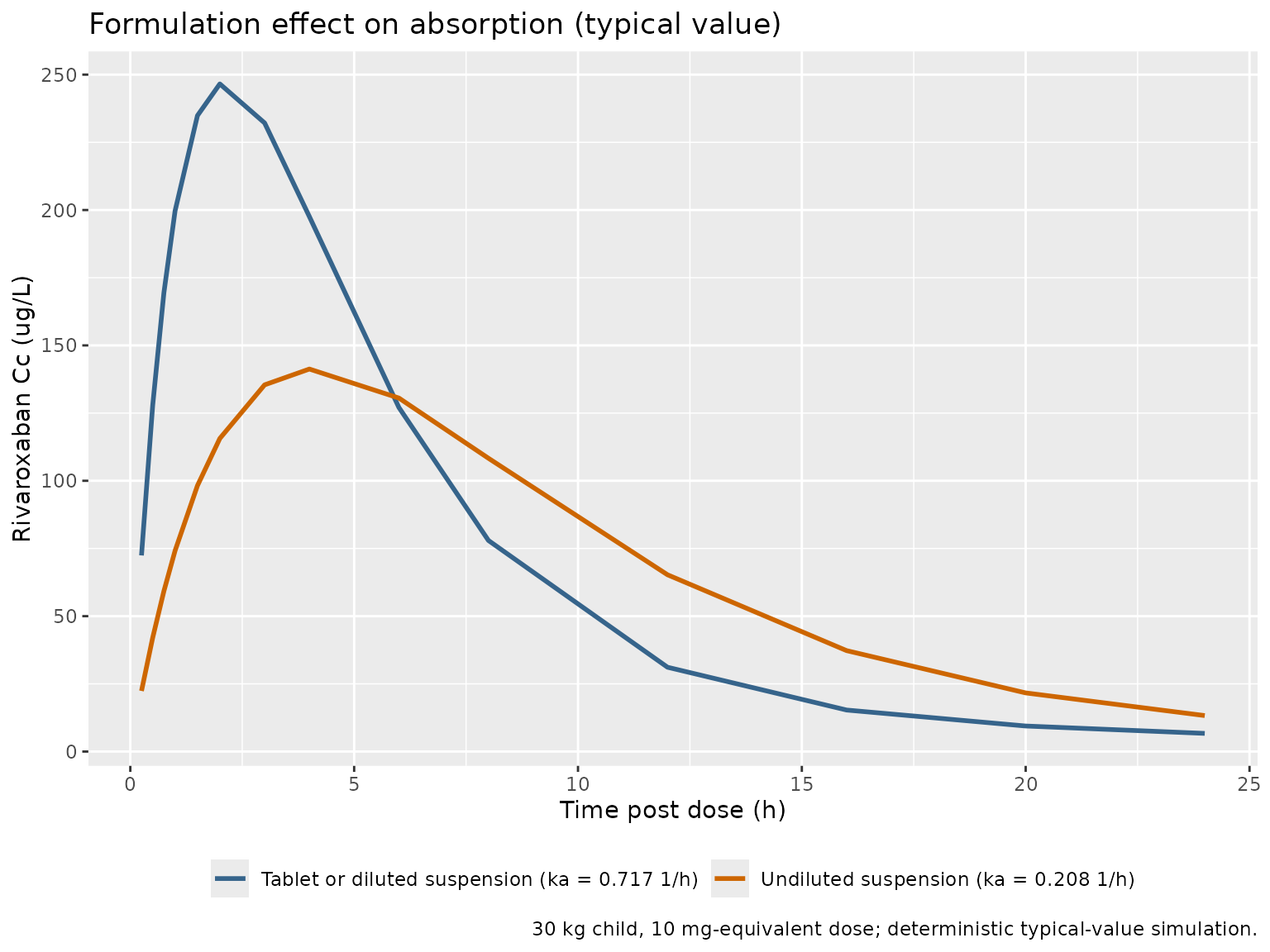
PKNCA validation
Compute Cmax, Tmax, AUC0-24, and C24h per simulated child, stratified
by the treatment label (age x dose cell). The popPK definitions in
Willmann 2018 Methods state that PopPK-derived Cmax is the absolute peak
of the concentration-time profile and C24h is the concentration exactly
24 h after dosing; the simulation grid here lands an observation at t =
24 so the PKNCA-derived ctau (with end = 24) corresponds to
C24h.
sim_nca <- sim |>
  dplyr::filter(!is.na(Cc)) |>
  dplyr::select(id, time, Cc, treatment)

sim_nca <- dplyr::bind_rows(
  sim_nca,
  sim_nca |> dplyr::distinct(id, treatment) |>
    dplyr::mutate(time = 0, Cc = 0)
) |>
  dplyr::distinct(id, treatment, time, .keep_all = TRUE) |>
  dplyr::arrange(id, treatment, time)

conc_obj <- PKNCA::PKNCAconc(sim_nca, Cc ~ time | treatment + id,
                             concu = "ug/L", timeu = "h")

dose_df <- events |>
  dplyr::filter(evid == 1L) |>
  dplyr::select(id, time, amt, treatment)

dose_obj <- PKNCA::PKNCAdose(dose_df, amt ~ time | treatment + id,
                             doseu = "mg")

intervals <- data.frame(
  start    = 0,
  end      = 24,
  cmax     = TRUE,
  tmax     = TRUE,
  auclast  = TRUE,
  clast.obs = TRUE
)

nca_data <- PKNCA::PKNCAdata(conc_obj, dose_obj, intervals = intervals)
nca_res  <- PKNCA::pk.nca(nca_data)
Comparison against Willmann 2018 Table 2 (PopPK column)
Willmann 2018 Table 2 reports the PopPK-derived geometric mean (with CV%) for AUC0-24, Cmax, and C24h per (age x dose x formulation) cohort. The published values are transcribed below; the simulated values are summarised over all subjects within each (age x dose) cell, ignoring formulation, for comparison.
published <- tibble::tribble(
  ~treatment,                ~cmax, ~auclast, ~ctau,
  "12-18y / 10 mg-eq",       129,   1320,     7.94,
  "12-18y / 20 mg-eq",       180,   1760,     9.46,
  "6-12y / 10 mg-eq",        118,    902,     3.18,   # Tablet 10 mg-eq cohort (n = 4)
  "6-12y / 20 mg-eq",        172,   1540,     8.46,   # Tablet 20 mg-eq cohort (n = 4)
  "2-6y / 10 mg-eq",         84.2,   674,     3.27,   # Suspension 10 mg-eq (n = 11)
  "2-6y / 20 mg-eq",         60.1,   755,     5.71,   # Suspension 20 mg-eq (n = 5)
  "0.5-2y / 10 mg-eq",       94.9,   503,     1.94,   # Suspension 10 mg-eq (n = 6)
  "0.5-2y / 20 mg-eq",       143,    672,     2.39    # Suspension 20 mg-eq (n = 4)
)

sim_nca_summary <- as.data.frame(nca_res) |>
  dplyr::filter(PPTESTCD %in% c("cmax", "auclast", "clast.obs")) |>
  dplyr::group_by(treatment, PPTESTCD) |>
  dplyr::summarise(
    sim_geomean = exp(mean(log(PPORRES), na.rm = TRUE)),
    sim_cv_pct  = 100 * sqrt(exp(stats::var(log(PPORRES), na.rm = TRUE)) - 1),
    .groups = "drop"
  )

sim_wide <- sim_nca_summary |>
  dplyr::select(treatment, PPTESTCD, sim_geomean) |>
  tidyr::pivot_wider(names_from = PPTESTCD, values_from = sim_geomean,
                     names_prefix = "sim_")

comparison <- published |>
  dplyr::left_join(sim_wide, by = "treatment") |>
  dplyr::mutate(
    cmax_sim     = round(sim_cmax, 1),
    auclast_sim  = round(sim_auclast, 0),
    ctau_sim     = round(`sim_clast.obs`, 2)
  ) |>
  dplyr::select(treatment, cmax, cmax_sim, auclast, auclast_sim,
                ctau, ctau_sim) |>
  dplyr::rename(
    "Treatment (age / dose-eq)" = treatment,
    "Cmax (paper, ug/L)"        = cmax,
    "Cmax (sim, ug/L)"          = cmax_sim,
    "AUC0-24 (paper, ug*h/L)"   = auclast,
    "AUC0-24 (sim, ug*h/L)"     = auclast_sim,
    "C24h (paper, ug/L)"        = ctau,
    "C24h (sim, ug/L)"          = ctau_sim
  )

knitr::kable(
  comparison,
  caption = "Simulated vs published (Willmann 2018 Table 2, PopPK column) geometric-mean NCA parameters.",
  align   = c("l", "r", "r", "r", "r", "r", "r")
)| Treatment (age / dose-eq) | Cmax (paper, ug/L) | Cmax (sim, ug/L) | AUC0-24 (paper, ug*h/L) | AUC0-24 (sim, ug*h/L) | C24h (paper, ug/L) | C24h (sim, ug/L) |
|---|---|---|---|---|---|---|
| 12-18y / 10 mg-eq | 129.0 | 142.4 | 1320 | 1268 | 7.94 | 7.52 |
| 12-18y / 20 mg-eq | 180.0 | 183.5 | 1760 | 1640 | 9.46 | 9.71 |
| 6-12y / 10 mg-eq | 118.0 | 184.1 | 902 | 1233 | 3.18 | 4.75 |
| 6-12y / 20 mg-eq | 172.0 | 245.6 | 1540 | 1692 | 8.46 | 7.12 |
| 2-6y / 10 mg-eq | 84.2 | 233.9 | 674 | 1311 | 3.27 | 5.17 |
| 2-6y / 20 mg-eq | 60.1 | 303.2 | 755 | 1677 | 5.71 | 6.46 |
| 0.5-2y / 10 mg-eq | 94.9 | 290.2 | 503 | 1301 | 1.94 | 5.24 |
| 0.5-2y / 20 mg-eq | 143.0 | 368.2 | 672 | 1678 | 2.39 | 6.75 |
The simulated values are computed from a virtual cohort whose dose-by-weight mapping is approximate (the EINSTEIN-Jr phase I per-weight dosing table is in the accompanying study publication, not in Willmann 2018). The general direction and magnitude of the simulated AUC, Cmax, and C24h should track the published PopPK column; large deviations (especially in the youngest cohorts where the dose-by-weight mapping is most uncertain) reflect dosing-table mismatch rather than a structural-model issue. See the Assumptions section below.
Assumptions and deviations
-
Dose-by-weight scheme. Willmann 2018 reports only
the “10 mg-equivalent” / “20 mg-equivalent” target labels; the
per-weight rivaroxaban mg amounts assigned in EINSTEIN-Jr phase I appear
in the accompanying clinical publication (reference 18 of Willmann
2018), which is not on disk for this extraction. The vignette uses
dose = nominal_eq_mg * (WT / 70)^0.323to approximate the dosing-design intent under the estimated allometric CL exponent; this matches the popPK exposures asymptotically but may diverge by ~10-20% from the actual study dose-by-weight table in the youngest cohorts. -
Formulation distribution within each cohort. The
vignette uses one representative formulation per (age x dose) cell
rather than the actual per-subject formulation distribution (which mixed
tablets, undiluted suspension, and diluted suspension in the 6-12 y
group; mixed undiluted and diluted suspension in the 2-6 y and 0.5-2 y
groups). A separate panel (“Formulation effect on absorption”) shows the
typical-value
kashift between the tablet / diluted-suspension and undiluted-suspension arms. - Cohort weight distributions. Age-cohort weights are sampled from age-appropriate normal distributions (means 10, 17, 30, 55 kg and SDs 1.5, 3, 6, 10 kg) chosen to approximate population norms for the four EINSTEIN-Jr age strata, with a 2.5 kg floor. The actual study weight distribution is in the accompanying clinical publication.
- Below-LLOQ handling. The popPK fit excluded 7 of 206 plasma concentrations as below the LLOQ of 0.500 ug/L (Willmann 2018 Results paragraph 1); the simulation does not censor below-LLOQ values because the parameter estimates are themselves the post-exclusion fit.
- No covariates beyond body weight, formulation, and dose level were retained in the final model. The paper reports that the allometric V exponent was estimated as not significantly different from 1 and was therefore fixed at 1 consistent with allometric theory; no race, sex, age, or covariate effects on CL / Vc / Q / Vp / F1 / ka are reported.
How to load the model
mod <- nlmixr2lib::readModelDb("Willmann_2018_rivaroxaban")
# inspect:
mod
# show metadata:
mod()$population