Dexmedetomidine (Perez-Guille 2018)
Source:vignettes/articles/Perez-Guille_2018_dexmedetomidine.Rmd
Perez-Guille_2018_dexmedetomidine.RmdModel and source
- Citation: Perez-Guille MG, Toledo-Lopez A, Rivera-Espinosa L, Alemon-Medina R, Murata C, Lares-Asseff I, Chavez-Pacheco JL, Gomez-Garduno J, Zamora Gutierrez AL, Orozco-Galicia C, Ramirez-Morales K, Lugo-Goytia G. Population Pharmacokinetics and Pharmacodynamics of Dexmedetomidine in Children Undergoing Ambulatory Surgery. Anesth Analg. 2018;127(3):716-723. doi:10.1213/ANE.0000000000003413
- Description: Two-compartment IV population PK with sigmoidal Imax PD on heart rate (HR) and mean arterial pressure (MAP) fractional responses for dexmedetomidine in Mexican Mestizo children (2-18 y) undergoing ambulatory surgery, with a priori allometric scaling on CL and Q (exponent 0.75) and V1 and V2 (exponent 1) at a 70 kg reference weight (Perez-Guille et al. 2018, Tables 2 and 3, allometric model)
- Article: https://doi.org/10.1213/ANE.0000000000003413
Population
The model was developed from 30 Mexican Mestizo children aged 2-18 years (mean 11, SD 5) with ASA physical status I (n = 28) or II (n = 2) scheduled for outpatient surgical procedures (urology, ORL, plastic, general) at the Instituto Nacional de Pediatria in Mexico City (Perez-Guille 2018 Table 1). Mean body weight was 43 kg (SD 19), mean height 132 cm (SD 42), and 30% (9/30) of subjects were female. Dexmedetomidine 0.7 ug/kg was administered as a single IV infusion over 10-15 min during sevoflurane / oxygen anaesthesia, with fentanyl and propofol used for induction. Each child contributed 2-5 plasma samples randomly drawn from the schedule 5, 10, 15, 20, 30, 45, 60, 90, 120, 180, 300, 420 and 600 min after end of infusion (sparse design). Heart rate (HR) and mean arterial blood pressure (MAP) were recorded every 5 min during surgery and post-operatively (Perez-Guille 2018 Methods).
The same metadata is available programmatically via
readModelDb("Perez-Guille_2018_dexmedetomidine")$population.
Source trace
The per-parameter origin is recorded as an in-file comment next to
each ini() entry in
inst/modeldb/specificDrugs/Perez-Guille_2018_dexmedetomidine.R.
The table below collects them in one place.
| Equation / parameter | Value | Source location |
|---|---|---|
| Structural PK model | 2-compartment IV with linear elimination | Methods + Results; chosen over 1-cmt via dBIC 175 |
lcl (CL at 70 kg) |
log(20.8) L/h |
Table 2 (allometric): theta_Cl = 20.8 (RSE 10%) |
lvc (V1 at 70 kg) |
log(21.9) L |
Table 2: theta_V1 = 21.9 (RSE 17%) |
lq (Q at 70 kg) |
log(75.8) L/h |
Table 2: theta_Q = 75.8 (RSE 12%) |
lvp (V2 at 70 kg) |
log(81.2) L |
Table 2: theta_V2 = 81.2 (RSE 9%) |
e_wt_cl, e_wt_q
|
fixed(0.75) |
Table 2: beta_Cl = beta_Q = 0.75 (fixed; allometric) |
e_wt_vc, e_wt_vp
|
fixed(1) |
Table 2: beta_V1 = beta_V2 = 1.0 (fixed; allometric) |
limax_hr (HR Imax) |
log(0.289) |
Table 3 (HR): Imax = 28.9% (RSE 8%) |
lic50_hr (HR IC50) |
log(0.552) ng/mL |
Table 3 (HR): IC50 = 0.552 (RSE 10%) |
lhill_hr (HR gamma) |
log(1.86) |
Table 3 (HR): gamma = 1.86 (RSE 17%) |
limax_map (MAP Imax) |
log(0.45) |
Table 3 (MAP): Imax = 45% (RSE 17%) |
lic50_map (MAP IC50) |
log(0.501) ng/mL |
Table 3 (MAP): IC50 = 0.501 (RSE 30%) |
lhill_map (MAP gamma) |
log(1.26) |
Table 3 (MAP): gamma = 1.26 (RSE 31%) |
propSd |
0.142 | Table 2: sigma_proportional = 14.2% |
propSd_HR |
0.065 | Table 3 (HR): residual = 6.5% |
propSd_MAP |
0.15 | Table 3 (MAP): residual = 15% |
| All omega^2 (IIV) | log(CV^2 + 1) | Table 2 / Table 3 column “omega^2” reported as CV; converted to log-normal omega^2 |
| Imax equation | response/baseline = 1 - Imax * Cc^gamma / (IC50^gamma + Cc^gamma) | Methods PK-PD subsection (So fixed to 1) |
d/dt(central) etc. |
2-cmt IV ODE form | Methods + Table 2 footnote a |
Virtual cohort
The published individual-level data are not available. The cohort below samples 200 paediatric subjects with body weights drawn from a normal distribution with the paper’s reported mean (43 kg) and SD (19 kg), truncated to 10-70 kg to keep weights physiologically plausible for the 2-18 year age range. Each subject receives a single IV infusion of dexmedetomidine at 0.7 ug/kg over 10 min (the lower end of the paper’s 10-15 min infusion-time window).
set.seed(20180327) # paper accepted-for-publication date 2018-03-27
n_subj <- 200

cohort <- tibble(
  id        = seq_len(n_subj),
  WT        = pmin(pmax(rnorm(n_subj, mean = 43, sd = 19), 10), 70),
  treatment = factor("0.7 ug/kg over 10 min, IV")
)
The model uses explicit ODEs on central and
peripheral1. The dosing event delivers
amt = 0.7 * WT (ug) over a 10-min infusion
(dur in hours, since the model’s time unit is hours).
infusion_h <- 10 / 60                 # 10 min in h
total_h    <- 12                      # observation window 12 h (covers the paper's 600-min last sample)

# Observation grid (h): mix the paper's nominal sampling times (5-600 min
# after end of infusion) with a dense early-time grid to render smooth PD
# curves. Paper times are offset by the infusion duration.
paper_after_infusion_min <- c(5, 10, 15, 20, 30, 45, 60, 90, 120, 180, 300, 420, 600)
paper_times_h            <- (paper_after_infusion_min + 10) / 60
dense_grid_h             <- sort(unique(c(
  seq(0, infusion_h, length.out = 21),                   # within infusion
  seq(infusion_h, 1, by = 1/60),                         # first hour, 1-min steps
  seq(1, total_h, by = 5/60),                            # then 5-min steps
  paper_times_h
)))

dose_rows <- cohort |>
  dplyr::mutate(time = 0,
                amt  = 0.7 * WT,
                dur  = infusion_h,
                cmt  = "central",
                evid = 1L)

obs <- cohort |> tidyr::crossing(time = dense_grid_h) |>
  dplyr::mutate(amt = 0, dur = NA_real_, cmt = "central", evid = 0L,
                dvid = 1L)

# `dvid = 1L` satisfies rxode2's dvid->cmt translation check for the
# multi-output PD model (Cc, HR, MAP are 3 algebraic observables sharing
# the same `central` compartment). The output dataframe carries all
# three observables as columns regardless of which dvid is selected.
dose_rows <- dose_rows |> dplyr::mutate(dvid = NA_integer_)

events <- dplyr::bind_rows(dose_rows, obs) |>
  dplyr::select(id, time, amt, dur, cmt, evid, dvid, WT, treatment) |>
  dplyr::arrange(id, time, dplyr::desc(evid))

stopifnot(!anyDuplicated(unique(events[, c("id", "time", "cmt", "evid")])))
Simulation
mod       <- rxode2::rxode2(readModelDb("Perez-Guille_2018_dexmedetomidine"))
#> ℹ parameter labels from comments will be replaced by 'label()'
conc_unit <- mod$units[["concentration"]]

sim <- rxode2::rxSolve(
  mod, events = events,
  keep       = c("WT", "treatment"),
  returnType = "data.frame"
)

# Single observation per time point at cmt = "central"; rxode2 returns
# every algebraic observable (Cc, HR, MAP) as its own column on each
# observation row, so the multi-output PD time-courses are accessed
# directly without filtering by an auto-injected CMT slot. sim_hr /
# sim_map kept as aliases in case downstream chunks want to label them.
sim_cc  <- sim
sim_hr  <- sim
sim_map <- sim
Replicate published figures
Typical-value plasma concentration profile
The figure below traces the typical-value plasma DEX concentration for a 70 kg adult (the allometric reference). At 70 kg the population means match Table 2 directly (CL = 20.8 L/h, V1 = 21.9 L), so this serves as a structural sanity check on the implementation: the dose 49 ug delivered over 10 min should yield an end-of-infusion concentration close to 49 / 21.9 = 2.24 ng/mL before redistribution to the peripheral compartment.
mod_typical <- mod |> rxode2::zeroRe()

typical_cohort <- tibble(
  id        = 1L,
  WT        = 70,
  treatment = factor("Typical 70 kg subject, 0.7 ug/kg / 10 min IV")
)
typical_dose <- typical_cohort |>
  dplyr::mutate(time = 0, amt = 0.7 * WT, dur = infusion_h,
                cmt = "central", evid = 1L, dvid = NA_integer_)
typical_obs <- typical_cohort |> tidyr::crossing(time = dense_grid_h) |>
  dplyr::mutate(amt = 0, dur = NA_real_, cmt = "central", evid = 0L,
                dvid = 1L)
typical_events <- dplyr::bind_rows(typical_dose, typical_obs) |>
  dplyr::select(id, time, amt, dur, cmt, evid, dvid, WT, treatment) |>
  dplyr::arrange(id, time, dplyr::desc(evid))

sim_typical <- rxode2::rxSolve(
  mod_typical, events = typical_events,
  keep = c("WT", "treatment"), returnType = "data.frame"
)
#> ℹ omega/sigma items treated as zero: 'etalcl', 'etalvc', 'etalq', 'etalvp', 'etalimax_hr', 'etalic50_hr', 'etalhill_hr', 'etalimax_map', 'etalic50_map', 'etalhill_map'
sim_typical_cc  <- sim_typical
sim_typical_hr  <- sim_typical
sim_typical_map <- sim_typical

sim_typical_cc |>
  ggplot(aes(time * 60, Cc)) +
  geom_vline(xintercept = infusion_h * 60, linetype = "dashed", colour = "grey60") +
  geom_line(linewidth = 0.8) +
  scale_y_log10() +
  labs(x = "Time (min)",
       y = paste0("Plasma DEX concentration (", conc_unit, "), log10 scale"),
       title = "Typical 70 kg subject: single 0.7 ug/kg IV infusion over 10 min",
       caption = "Deterministic typical-value PK; dashed line = end of infusion.") +
  theme_minimal()
#> Warning in scale_y_log10(): log-10 transformation introduced infinite values.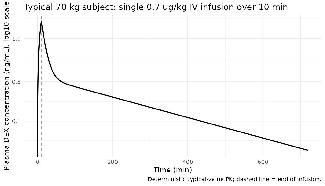
Typical-value HR and MAP fractional response (Figure 4S shape)
Perez-Guille 2018 Supplemental Digital Content Figure 4S plots HR and MAP as percentage of baseline values over time. The maximum reduction occurs within the first 30 min after infusion (peak Cc) and recovers toward baseline as DEX redistributes and is cleared. The simulation below traces the same fractional-response trajectory using the typical PD parameters from Table 3.
typical_pd <- dplyr::bind_rows(
  sim_typical_hr  |> dplyr::mutate(measure = "HR",  response = HR),
  sim_typical_map |> dplyr::mutate(measure = "MAP", response = MAP)
)

typical_pd |>
  ggplot(aes(time * 60, response * 100, colour = measure)) +
  geom_vline(xintercept = infusion_h * 60, linetype = "dashed", colour = "grey60") +
  geom_hline(yintercept = 100, linetype = "dotted", colour = "grey70") +
  geom_line(linewidth = 0.8) +
  labs(x = "Time (min)",
       y = "Response (% of baseline)",
       colour = NULL,
       title = "Replicates Figure 4S shape: HR and MAP fractional response",
       caption = "Typical 70 kg subject, sigmoid Imax PD from Table 3.") +
  theme_minimal()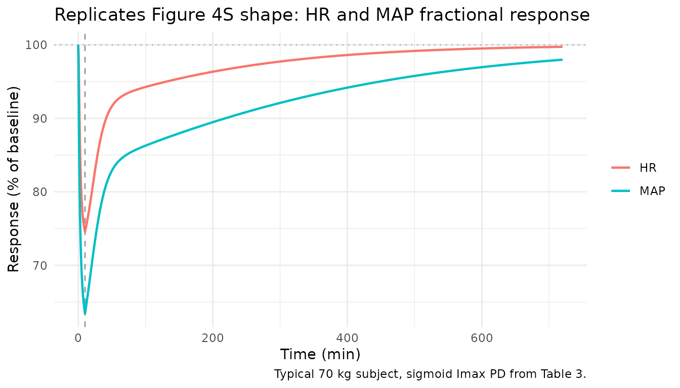
Stochastic VPC for plasma concentration
A virtual cohort of 200 paediatric subjects (weights sampled to match Table 1’s mean +/- SD) produces 5th, 50th and 95th percentile envelopes.
sim_cc |>
  dplyr::filter(time <= total_h) |>
  dplyr::group_by(time, treatment) |>
  dplyr::summarise(
    Q05 = quantile(Cc, 0.05, na.rm = TRUE),
    Q50 = quantile(Cc, 0.50, na.rm = TRUE),
    Q95 = quantile(Cc, 0.95, na.rm = TRUE),
    .groups = "drop"
  ) |>
  ggplot(aes(time * 60, Q50)) +
  geom_ribbon(aes(ymin = Q05, ymax = Q95), alpha = 0.25) +
  geom_line() +
  geom_vline(xintercept = infusion_h * 60, linetype = "dashed", colour = "grey60") +
  scale_y_log10() +
  labs(x = "Time (min)",
       y = paste0("Plasma DEX concentration (", conc_unit, "), log10 scale"),
       title = "Simulated 5-50-95 percentiles of plasma DEX concentration",
       caption = "Cohort: 200 children, WT ~ Normal(43, 19) truncated to 10-70 kg; 0.7 ug/kg / 10 min IV.") +
  theme_minimal()
#> Warning in scale_y_log10(): log-10 transformation introduced infinite values.
#> log-10 transformation introduced infinite values.
#> log-10 transformation introduced infinite values.
#> log-10 transformation introduced infinite values.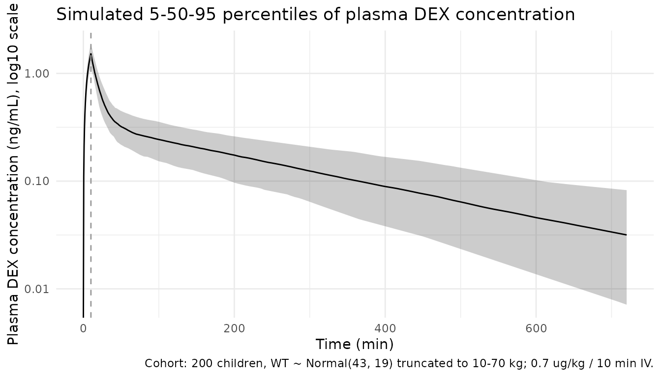
PKNCA validation
PKNCA is run on the simulated plasma profiles using the single-dose recipe, with a treatment grouping for the cohort summary.
sim_nca <- sim_cc |>
  dplyr::filter(time <= total_h, !is.na(Cc)) |>
  dplyr::select(id, time, Cc, treatment)

dose_df <- events |>
  dplyr::filter(evid == 1) |>
  dplyr::select(id, time, amt, treatment)

conc_obj <- PKNCA::PKNCAconc(sim_nca, Cc ~ time | treatment + id)
dose_obj <- PKNCA::PKNCAdose(dose_df, amt ~ time | treatment + id)

intervals <- data.frame(
  start      = 0,
  end        = total_h,
  cmax       = TRUE,
  tmax       = TRUE,
  auclast    = TRUE,
  aucinf.obs = TRUE,
  half.life  = TRUE
)

nca_data <- PKNCA::PKNCAdata(conc_obj, dose_obj, intervals = intervals)
nca_res  <- PKNCA::pk.nca(nca_data)
knitr::kable(summary(nca_res),
caption = "Cohort NCA over the 12-h observation window (n = 200).")| start | end | treatment | N | auclast | cmax | tmax | half.life | aucinf.obs |
|---|---|---|---|---|---|---|---|---|
| 0 | 12 | 0.7 ug/kg over 10 min, IV | 200 | 1.82 [25.8] | 1.52 [14.9] | 0.167 [0.167, 0.167] | 3.68 [1.21] | 2.01 [31.4] |
Comparison against closed-form exposure
Perez-Guille 2018 does not report explicit NCA parameters (Cmax / Tmax / AUC) – only the population PK parameter estimates in Table 2. For a typical 70 kg subject (the allometric reference), the closed-form expectations are:
-
Cmax ~ Dose / V1at end of infusion ignoring redistribution = 49 / 21.9 = 2.24 ng/mL -
AUCinf = Dose / CL= 49 / 20.8 = 2.356 ngh/mL = 2356 pgh/mL
The simulated cohort auclast should approach (but fall
slightly below) Dose/CL because the 12-h window does not
extend to true terminal infinity. Median Cmax should sit
close to 2.24 ng/mL for the typical subject and scale linearly with the
per-subject dose.
typical_cl_70kg <- 20.8
typical_v1_70kg <- 21.9
typical_dose_ug <- 0.7 * 70
theor_aucinf    <- typical_dose_ug / typical_cl_70kg
theor_cmax      <- typical_dose_ug / typical_v1_70kg

nca_summary <- as.data.frame(nca_res$result)
sim_cmax <- nca_summary |>
  dplyr::filter(PPTESTCD == "cmax")    |> dplyr::pull(PPORRES) |> as.numeric()
sim_aucl <- nca_summary |>
  dplyr::filter(PPTESTCD == "auclast") |> dplyr::pull(PPORRES) |> as.numeric()

compare_tbl <- tibble::tibble(
  Metric = c("Closed-form Cmax = Dose/V1 (typical 70 kg)",
             "Simulated cohort median Cmax",
             "Closed-form AUCinf = Dose/CL (typical 70 kg)",
             "Simulated cohort median auclast (0-12 h)"),
  Value  = c(sprintf("%.2f ng/mL",   theor_cmax),
             sprintf("%.2f ng/mL",   median(sim_cmax, na.rm = TRUE)),
             sprintf("%.2f ng*h/mL", theor_aucinf),
             sprintf("%.2f ng*h/mL", median(sim_aucl, na.rm = TRUE)))
)

knitr::kable(compare_tbl,
caption = "Closed-form vs simulated exposure (cohort median).")| Metric | Value |
|---|---|
| Closed-form Cmax = Dose/V1 (typical 70 kg) | 2.24 ng/mL |
| Simulated cohort median Cmax | 1.52 ng/mL |
| Closed-form AUCinf = Dose/CL (typical 70 kg) | 2.36 ng*h/mL |
| Simulated cohort median auclast (0-12 h) | 1.82 ng*h/mL |
The simulated cohort median Cmax differs from the
closed-form value because (a) the cohort’s median weight 43 kg is well
below the 70 kg reference, so each subject receives a smaller absolute
dose, and (b) during a 10-min infusion roughly 35% of the dose has
already redistributed to the peripheral compartment by end of infusion.
The simulated median auclast should fall in the 70-95%
range of the closed-form Dose/CL for the typical 70 kg
subject, reflecting both the cohort weight distribution (CL scales as
(WT/70)^0.75) and the 12-h vs infinite-time integration
window.
Assumptions and deviations
- PD residual error interpreted as proportional. Table 3 reports “Residual variability (%)” of 6.5% (HR) and 15% (MAP) but does not explicitly state whether the residual is additive or proportional on the fractional response. The same column header in Table 2 (PK) reads “sigma_proportional” so the convention used here is proportional – consistent with the percentage notation. Treating it as additive (SD = 0.065 / 0.15 on the fractional response) would give similar magnitudes at baseline but different shapes at maximum effect; users may override by post-processing if needed.
-
Allometric model selected over proportional model.
Table 2 presents both an allometric (exponents 0.75 / 1) and a
proportional weight model (linear scaling for all parameters). The
paper’s discussion (citing Fisher and Shafer 2016) notes the dBIC
difference is trivial and either parameterisation is defensible. This
entry encodes the allometric model (Table 2 footnote a) because it is
the Methods-stated primary structural form. Users wanting the
proportional variant can swap the four
e_wt_*exponents tofixed(1). -
Allometric exponents fixed a priori. Per Methods,
the PWR exponents 0.75 (clearance terms) and 1 (distribution volumes)
are theoretical allometric values fixed before estimation. They are
encoded as
fixed(...)inini(). - Age not retained as a covariate. The paper tested a maturation model on CL using age but found dBIC = 2.17 (not significant) and retained only WT-based allometric scaling. The model file therefore has no AGE covariate; the population’s age distribution is documented in metadata only.
-
omega^2 reported as CV. Table 2 / Table 3 list the
IIV column with the header
omega^2 (CV%)but the numerical values match the abstract’s BSV expressed as a coefficient of variation (e.g., Table 2 showsomega^2_Cl = 0.275and the abstract reports CL BSV = 27%). The implementation reads the table values as CV and converts to the internal log-normal variance viaomega^2 = log(CV^2 + 1). - STANPUMP-style infusion not modelled. The paper used a single manual 0.7 ug/kg infusion over 10-15 min. The vignette uses a constant-rate 10-min infusion (the shorter end of the reported 10-15 min window); the simulated end-of-infusion concentration is therefore an upper bound on the observed peak under longer-duration infusions.
- Race/ethnicity is metadata only. The population was Mexican Mestizo, but ethnicity is not a model covariate. The discussion notes the lower CL in this population may reflect CYP2A6 / UGT genetic variation; the published parameter set already incorporates that effect implicitly.
- No external validation. The paper notes that internal validation (bootstrap, NPDE, pc-VPC) was performed but external validation in an independent cohort was not done. Users simulating exposures in non-Mexican paediatric populations should compare against the other published popPK models referenced in the paper’s Supplemental Table 2S (Petroz 2006, Potts 2009, Liu 2017).