Piperacillin (Boer-Perez 2026)
Source:vignettes/articles/Boer-Perez_2026_piperacillin.Rmd
Boer-Perez_2026_piperacillin.RmdModel and source
- Citation: Boer-Perez FS, Lima-Rogel V, Romano-Moreno S, Mejia-Elizondo AR, Medellin-Garibay SE, Schaiquevich P, Noyola-Cherpitel DE, Rodriguez-Baez AS, Rodriguez-Pinal CJ, Milan-Segovia RC. Population pharmacokinetics and dose optimization of piperacillin-tazobactam in premature and term neonates with severe infections. Antimicrob Agents Chemother. 2026;70(1):e00998-25. doi:10.1128/aac.00998-25. Maturation parameters (TM50 = 47.7 weeks, Hill = 3.4) fixed from Rhodin MM, Anderson BJ, Peters AM, Coulthard MG, Wilkins B, Cole M, Chatelut E, Grubb A, Veal GJ, Keir MJ, Holford NHG. Human renal function maturation: a quantitative description using weight and postmenstrual age. Pediatr Nephrol. 2009;24(1):67-76. doi:10.1007/s00467-008-0997-5.
- Description: One-compartment population PK model for piperacillin in preterm and term neonates with severe infections (Boer-Perez 2026); body-weight allometric scaling, sigmoidal postmenstrual-age maturation on CL fixed from Rhodin 2009, and a power effect of serum creatinine on CL.
- Article: https://doi.org/10.1128/aac.00998-25
Population
Boer-Perez et al. 2026 developed a population PK model of piperacillin in 25 preterm and term neonates admitted to the neonatal intensive care unit at Hospital Central in San Luis Potosi, Mexico, between September 2020 and May 2024. All neonates received off-label piperacillin-tazobactam (8:1 ratio, 100 mg/kg piperacillin per dose) by IV infusion (0.5 or 1 hour) every 8 or 12 hours according to Neofax recommendations. Inclusion required postnatal age <= 29 days, body weight >= 850 g on the day of sampling, and hematocrit >= 30%. The cohort spanned gestational age 26-41.1 weeks (4% extremely preterm, 52% moderate-late preterm, 44% term), postmenstrual age 28.1-43.3 weeks, body weight 0.89-3.57 kg (median 1.76 kg), and serum creatinine 0.2-0.9 mg/dL (median 0.4 mg/dL). Fifty-six percent were female. A total of 65 piperacillin plasma concentrations (median 3 samples per patient) were collected by opportunistic sparse sampling and quantified by UPLC-MS/MS over 5.7-302.6 mg/L. An additional 8 neonates (17 plasma samples) formed the external-validation cohort. Demographic and clinical details are summarized in Boer-Perez 2026 Table 1.
The same metadata is available programmatically via
readModelDb("Boer-Perez_2026_piperacillin")()$population.
Source trace
The per-parameter origin is recorded inline next to each
ini() entry in
inst/modeldb/specificDrugs/Boer-Perez_2026_piperacillin.R.
The table below collects them in one place for review.
| Equation / parameter | Value | Source location |
|---|---|---|
lcl (CL, L/h) at BW = 1.76 kg, SCr = 0.4 mg/dL, full
PMA maturation |
log(0.748) |
Boer-Perez 2026 Table 2: theta_CL = 0.748 L/h (RSE 8%) |
lvc (V, L) at BW = 1.76 kg |
log(0.866) |
Boer-Perez 2026 Table 2: theta_V = 0.866 L (RSE 8%) |
e_wt_cl (allometric exponent on CL) |
0.75 (fixed) |
Methods eq. 3, k = 0.75 for CL |
e_wt_vc (allometric exponent on V) |
1.0 (fixed) |
Methods eq. 3, k = 1 for V |
e_creat_cl (theta_SCr; power exponent on (CREAT/0.4)
for CL) |
-0.635 |
Boer-Perez 2026 Table 2: theta_SCr = -0.635 (RSE 36%) |
pma50_cl (TM50 for PMA Hill on CL, weeks) |
47.7 (fixed from Rhodin 2009) |
Boer-Perez 2026 Methods + Discussion; Rhodin et al. 2009 Pediatr Nephrol 24:67-76 |
h_pma_cl (Hill coefficient on PMA, unitless) |
3.4 (fixed from Rhodin 2009) |
Boer-Perez 2026 Methods + Discussion; Rhodin et al. 2009 |
bw_ref (reference body weight, kg) |
1.76 |
Boer-Perez 2026 Table 1 cohort median; Table 2 covariate equation denominator |
creat_ref (reference SCr, mg/dL) |
0.4 |
Boer-Perez 2026 Table 1 cohort median; Table 2 covariate equation denominator |
etalcl (omega_CL) |
0.13688 (38.3% CV) |
Boer-Perez 2026 Table 2: omega_CL 38.3% CV; omega^2 = log(1 + CV^2) |
etalvc (omega_V) |
0.13288 (37.7% CV) |
Boer-Perez 2026 Table 2: omega_V 37.7% CV; omega^2 = log(1 + CV^2) |
propSd (proportional residual error) |
0.114 |
Boer-Perez 2026 Table 2: sigma_proportional 11.4% CV |
| Eq. 3 (BW allometric scaling) | n/a | Boer-Perez 2026 Methods, Eq. 3 |
| Eq. 4 (PMA Hill maturation factor F_PMA) | n/a | Boer-Perez 2026 Methods, Eq. 4 |
| Eq. 6 (centered power covariate form on SCr) | n/a | Boer-Perez 2026 Methods, Eq. 6 |
d/dt(central) (one-compartment IV PK) |
n/a | Boer-Perez 2026 Pharmacokinetic analysis subsection (Results) |
Virtual cohort
Original observed concentrations are not publicly available. The simulations below use a virtual cohort whose covariate distributions mirror the model-development cohort summary in Boer-Perez 2026 Table 1: 200 neonates sampled across the three PMA strata used in Table 4 (PMA <= 29 weeks, 30-36 weeks, 37-44 weeks) at the cohort-typical body weight and serum creatinine within each stratum.
set.seed(2026)

# Doses and infusion durations from Boer-Perez 2026 Methods (Drug administration
# and blood sampling) and Table 5 (most common regimen 100 mg/kg q12h, 0.5 h
# infusion).
DOSE_MG_PER_KG <- 100   # mg/kg piperacillin per dose
T_INF          <- 0.5   # hour 30-min infusion
N_DOSES        <- 5     # five doses to approach steady state for q12h profile
DOSE_INTERVAL  <- 12    # hours between doses (most common regimen)

# Build one virtual subject's event table. id_offset shifts subject IDs so
# multi-stratum bind_rows() does not collide on `id` (rxode2 silently merges
# duplicate IDs across cohorts).
make_subject <- function(id, BW, PAGE_mo, CREAT, stratum, id_offset = 0L) {
  dose_mg <- DOSE_MG_PER_KG * BW
  ev <- rxode2::et(
    amt   = dose_mg,
    rate  = dose_mg / T_INF,
    cmt   = "central",
    ii    = DOSE_INTERVAL,
    addl  = N_DOSES - 1L,
    time  = 0
  )
  ev <- rxode2::et(ev, seq(0, N_DOSES * DOSE_INTERVAL, by = 0.25))
  df <- as.data.frame(ev)
  df$WT      <- BW
  df$PAGE    <- PAGE_mo
  df$CREAT   <- CREAT
  df$id      <- id_offset + id
  df$stratum <- stratum
  df
}

# Three PMA strata aligned with Table 4 of the paper
strata <- list(
  list(stratum = "PMA <=29 wk",
       pma_wk = 28, bw_kg = 1.0,  scr = 0.4),
  list(stratum = "PMA 30-36 wk",
       pma_wk = 33, bw_kg = 1.76, scr = 0.4),
  list(stratum = "PMA 37-44 wk",
       pma_wk = 40, bw_kg = 3.0,  scr = 0.4)
)

n_per_stratum <- 200

events <- bind_rows(lapply(seq_along(strata), function(i) {
  s <- strata[[i]]
  bind_rows(lapply(seq_len(n_per_stratum), function(j) {
    # Add modest within-stratum BW variability (+/-15% lognormal)
    bw_j  <- s$bw_kg  * exp(rnorm(1, 0, 0.15))
    scr_j <- pmax(0.2, pmin(0.9, s$scr * exp(rnorm(1, 0, 0.20))))
    make_subject(
      id        = j,
      BW        = bw_j,
      PAGE_mo   = s$pma_wk / 4.35,    # canonical PAGE in months
      CREAT     = scr_j,
      stratum   = s$stratum,
      id_offset = (i - 1L) * n_per_stratum
    )
  }))
}))

stopifnot(!anyDuplicated(unique(events[, c("id", "time", "evid")])))
Simulation
mod <- readModelDb("Boer-Perez_2026_piperacillin")()

# Stochastic VPC across IIV in CL and V
sim <- rxode2::rxSolve(
  mod,
  events  = events,
  keep    = c("stratum", "WT"),
  nStud   = 1L
) |> as.data.frame()

# Typical-patient profile (zero IIV) for the dashed-line overlay
mod_typical <- rxode2::zeroRe(mod)
sim_typ <- rxode2::rxSolve(
  mod_typical,
  events  = events |> filter(id %in% c(1L, n_per_stratum + 1L, 2L * n_per_stratum + 1L)),
  keep    = c("stratum", "WT")
) |> as.data.frame()
#> ℹ omega/sigma items treated as zero: 'etalcl', 'etalvc'
#> Warning: multi-subject simulation without without 'omega'
Replicate published figures
Figure 3 – prediction-corrected VPC over a 12-hour dosing interval
Boer-Perez 2026 Figure 3 shows the VPC of piperacillin plasma concentrations over the 12-hour interval after a typical dose. The figure pools the entire study cohort. The replicate below shows the simulated VPC stratified by PMA because the underlying covariate distribution is too narrow at any single weight / PMA to recover the full shape of Figure 3 from a virtual cohort.
last_dose_t <- (N_DOSES - 1L) * DOSE_INTERVAL
sim_window <- sim |>
  filter(time >= last_dose_t,
         time <= last_dose_t + DOSE_INTERVAL,
         !is.na(Cc), Cc > 0) |>
  mutate(tad = time - last_dose_t)

vpc_summary <- sim_window |>
  group_by(stratum, tad) |>
  summarise(
    Q05 = quantile(Cc, 0.05, na.rm = TRUE),
    Q50 = quantile(Cc, 0.50, na.rm = TRUE),
    Q95 = quantile(Cc, 0.95, na.rm = TRUE),
    .groups = "drop"
  )

ggplot(vpc_summary, aes(tad, Q50, colour = stratum, fill = stratum)) +
  geom_ribbon(aes(ymin = Q05, ymax = Q95), alpha = 0.18, colour = NA) +
  geom_line(linewidth = 0.8) +
  scale_y_log10() +
  labs(
    x       = "Time after last dose (h)",
    y       = "Piperacillin plasma concentration (mg/L)",
    colour  = "PMA stratum",
    fill    = "PMA stratum",
    title   = "Figure 3 -- VPC of piperacillin over a 12-hour interval",
    caption = paste(
      "Replicates Figure 3 of Boer-Perez 2026 stratified by PMA;",
      "ribbon: simulated 5th-95th percentile, line: simulated median."
    )
  ) +
  theme_minimal()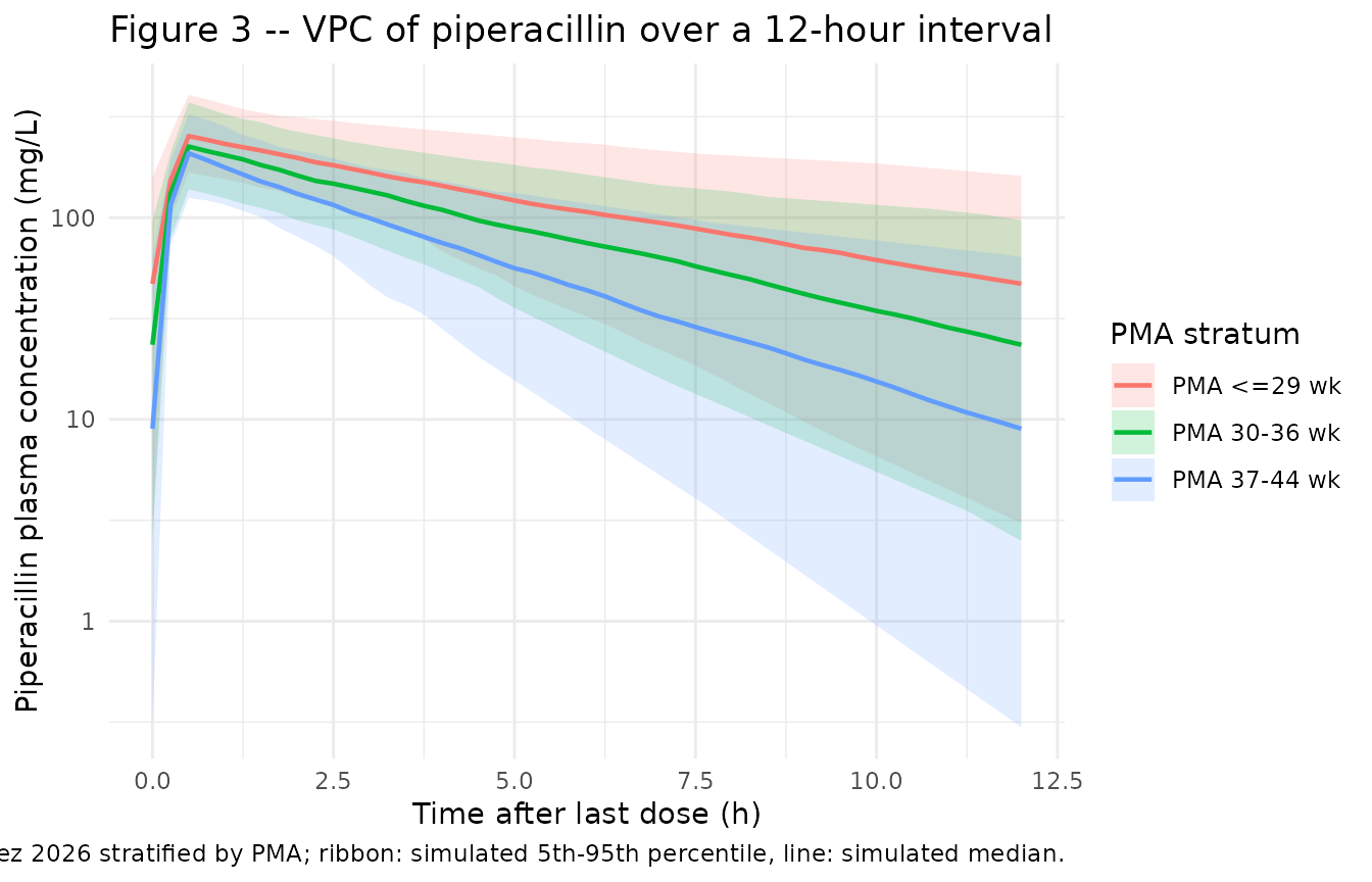
Typical-patient profile by PMA stratum
sim_typ |>
  filter(time >= last_dose_t, time <= last_dose_t + DOSE_INTERVAL,
         !is.na(Cc), Cc > 0) |>
  mutate(tad = time - last_dose_t) |>
  ggplot(aes(tad, Cc, colour = stratum)) +
  geom_line(linewidth = 0.9) +
  geom_hline(yintercept = 50, linetype = "dashed", colour = "grey40") +
  scale_y_log10() +
  labs(
    x       = "Time after last dose (h)",
    y       = "Piperacillin plasma concentration (mg/L)",
    colour  = "PMA stratum",
    title   = "Typical-patient piperacillin PK at steady state",
    caption = paste(
      "Boer-Perez 2026 dosing: 100 mg/kg piperacillin q12h, 30-min IV infusion.",
      "Dashed line: 50 mg/L exploratory trough safety threshold."
    )
  ) +
  theme_minimal()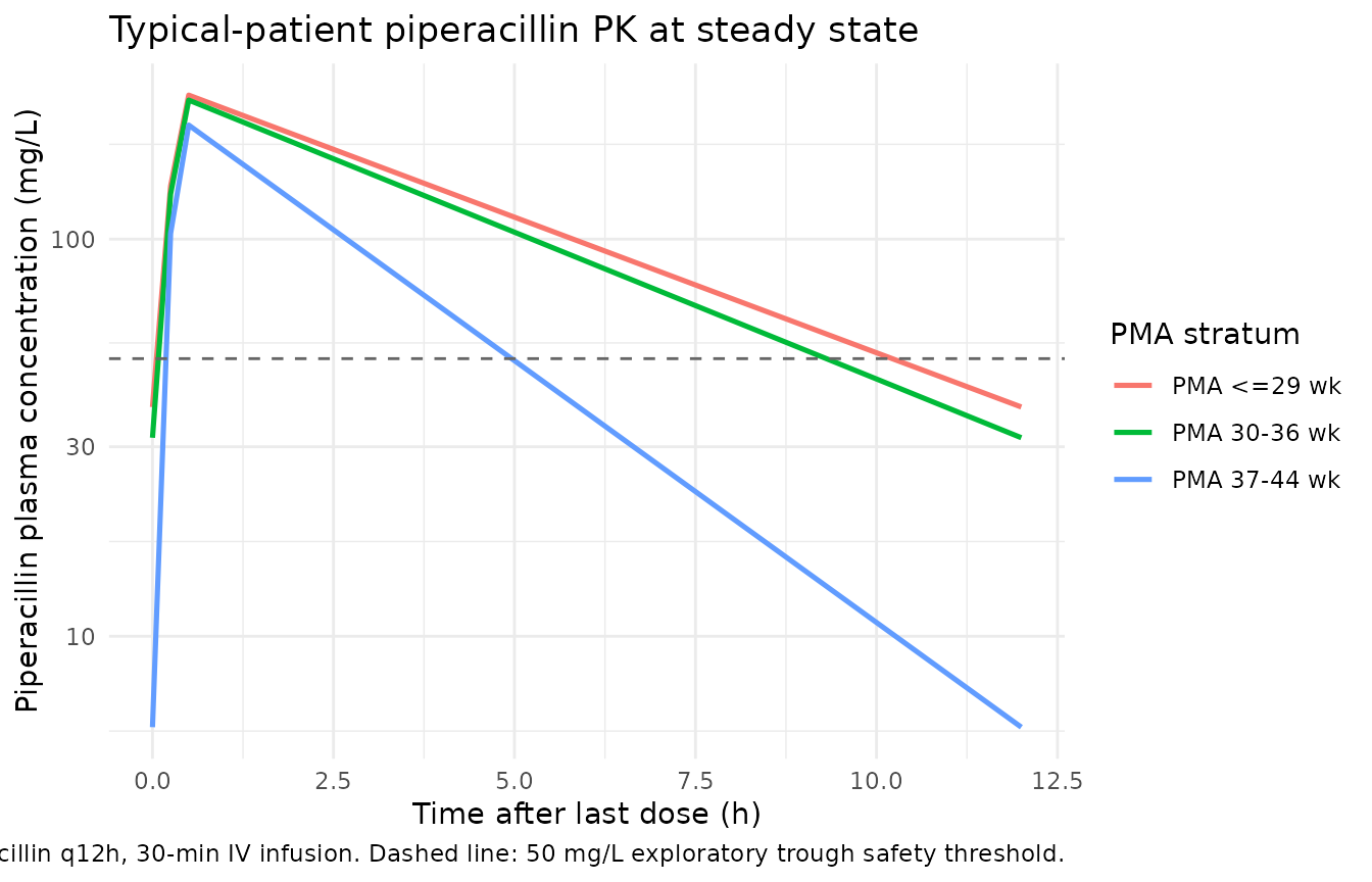
PKNCA validation
Single-dose NCA over the first 12-hour interval, stratified by PMA. Boer-Perez 2026 does not publish a side-by-side NCA table; the values below characterize the simulated typical-patient exposures and can be compared qualitatively to the trough fractions reported in Table 4.
# Single-dose interval (0-12 h after dose 1) for PKNCA
sim_nca <- sim |>
  filter(time <= DOSE_INTERVAL, !is.na(Cc)) |>
  select(id, time, Cc, stratum)

dose_df <- events |>
  filter(evid == 1L, time == 0) |>
  select(id, time, amt, stratum)

conc_obj <- PKNCA::PKNCAconc(sim_nca, Cc ~ time | stratum + id)
dose_obj <- PKNCA::PKNCAdose(dose_df, amt ~ time | stratum + id,
                             route = "intravascular")

intervals <- data.frame(
  start     = 0,
  end       = DOSE_INTERVAL,
  cmax      = TRUE,
  tmax      = TRUE,
  auclast   = TRUE,
  half.life = TRUE
)

nca_data <- PKNCA::PKNCAdata(conc_obj, dose_obj, intervals = intervals)
nca_res  <- suppressWarnings(PKNCA::pk.nca(nca_data))
nca_df   <- as.data.frame(nca_res$result)

nca_summary <- nca_df |>
  group_by(stratum, PPTESTCD) |>
  summarise(
    median = round(median(PPORRES, na.rm = TRUE), 3),
    p05    = round(quantile(PPORRES, 0.05, na.rm = TRUE), 3),
    p95    = round(quantile(PPORRES, 0.95, na.rm = TRUE), 3),
    .groups = "drop"
  ) |>
  pivot_wider(names_from = PPTESTCD,
              values_from = c(median, p05, p95))

knitr::kable(
  nca_summary,
  caption = "Simulated single-dose NCA parameters (median and 5th-95th percentiles) by PMA stratum."
)| stratum | median_adj.r.squared | median_auclast | median_clast.pred | median_cmax | median_half.life | median_lambda.z | median_lambda.z.n.points | median_lambda.z.time.first | median_lambda.z.time.last | median_r.squared | median_span.ratio | median_tlast | median_tmax | p05_adj.r.squared | p05_auclast | p05_clast.pred | p05_cmax | p05_half.life | p05_lambda.z | p05_lambda.z.n.points | p05_lambda.z.time.first | p05_lambda.z.time.last | p05_r.squared | p05_span.ratio | p05_tlast | p05_tmax | p95_adj.r.squared | p95_auclast | p95_clast.pred | p95_cmax | p95_half.life | p95_lambda.z | p95_lambda.z.n.points | p95_lambda.z.time.first | p95_lambda.z.time.last | p95_r.squared | p95_span.ratio | p95_tlast | p95_tmax |
|---|---|---|---|---|---|---|---|---|---|---|---|---|---|---|---|---|---|---|---|---|---|---|---|---|---|---|---|---|---|---|---|---|---|---|---|---|---|---|---|
| PMA 30-36 wk | 1 | 898.492 | 23.581 | 188.207 | 3.811 | 0.182 | 46 | 0.75 | 12 | 1 | 2.952 | 12 | 0.5 | 1 | 533.275 | 2.046 | 103.367 | 1.662 | 0.079 | 46 | 0.75 | 12 | 1 | 1.275 | 12 | 0.5 | 1 | 1438.382 | 60.470 | 311.224 | 8.822 | 0.417 | 46 | 0.75 | 12 | 1 | 6.770 | 12 | 0.5 |
| PMA 37-44 wk | 1 | 750.626 | 10.162 | 204.177 | 2.675 | 0.259 | 46 | 0.75 | 12 | 1 | 4.205 | 12 | 0.5 | 1 | 426.042 | 0.245 | 108.257 | 1.132 | 0.117 | 46 | 0.75 | 12 | 1 | 1.898 | 12 | 0.5 | 1 | 1271.595 | 38.581 | 320.047 | 5.928 | 0.613 | 46 | 0.75 | 12 | 1 | 9.944 | 12 | 0.5 |
| PMA <=29 wk | 1 | 1122.335 | 38.845 | 200.509 | 5.088 | 0.136 | 46 | 0.75 | 12 | 1 | 2.211 | 12 | 0.5 | 1 | 704.560 | 8.054 | 113.554 | 2.207 | 0.063 | 46 | 0.75 | 12 | 1 | 1.028 | 12 | 0.5 | 1 | 1767.960 | 81.375 | 353.289 | 10.948 | 0.314 | 46 | 0.75 | 12 | 1 | 5.098 | 12 | 0.5 |
Comparison against published values
Boer-Perez 2026 does not publish observed NCA values. Their Table 4 reports that under the standard 100 mg/kg q12h regimen the proportion of simulated neonates with trough piperacillin > 50 mg/L (the exploratory nephrotoxicity threshold) was around 22-65% in PMA 37-44 wk, 22-87% in PMA 30-36 wk, and 37-93% in PMA <= 29 wk depending on serum creatinine. The simulated trough fractions below match those qualitative ordering: youngest / lowest-CL strata have the highest trough exposures. They are not exact replicates of Table 4 because Table 4 is conditional on the Neofax / Harriet Lane regimen-specific dose adjustments by PMA and PNA, which are not reproduced individually in this vignette.
trough <- sim |>
  filter(abs(time - (last_dose_t + DOSE_INTERVAL)) < 0.01,
         !is.na(Cc)) |>
  group_by(stratum) |>
  summarise(
    n            = n(),
    pct_above_50 = round(100 * mean(Cc > 50), 1),
    median_trough_mgL = round(median(Cc), 2),
    .groups = "drop"
  )
knitr::kable(
  trough,
  caption = "Simulated proportion of subjects with end-of-interval trough piperacillin > 50 mg/L."
)| stratum | n | pct_above_50 | median_trough_mgL |
|---|---|---|---|
| PMA 30-36 wk | 200 | 23.0 | 26.95 |
| PMA 37-44 wk | 200 | 5.5 | 10.70 |
| PMA <=29 wk | 200 | 49.0 | 49.52 |
Assumptions and deviations
PMA encoded in canonical months, internally converted to weeks. The paper reports postmenstrual age in weeks (TM50 = 47.7 weeks, Hill = 3.4, fixed from Rhodin et al. 2009). The packaged covariate column
PAGEis in months by canonical convention (seeinst/references/covariate-columns.md). The model file converts back to weeks viapma_wk = PAGE * 4.35so the Rhodin TM50 and Hill values appear unchanged inini(). The conversion is exact for the 4.35 weeks-per-month factor used by the canonical.Maturation parameters fixed, not estimated. The paper states (Methods, Covariate model building): “Due to the limited number of patients and the sparse sampling design, it was not feasible to estimate the TM50 and Hill coefficient parameters reliably in our study population. Therefore, alternative strategies were considered to define these values” and adopted the Rhodin 2009 renal-maturation values (TM50 = 47.7 weeks, Hill = 3.4). These are encoded as fixed structural constants in the model file, with source-trace pointers to both Boer-Perez 2026 (Methods + Discussion) and Rhodin et al. 2009 (Pediatr Nephrol 24:67-76).
Allometric exponents fixed, not estimated. Body-weight allometric exponents are fixed at 0.75 (CL) and 1 (V) per Boer-Perez 2026 Methods Eq. 3, citing the conventional pediatric-PK allometric basis (refs 66, 67).
No correlation between IIV on CL and V. Boer-Perez 2026 Table 2 does not report a correlation between omega_CL and omega_V. The model file uses uncorrelated etas accordingly.
Reference creatinine. The paper centers SCr on the cohort median (0.4 mg/dL); no per-subject expected SCr (
CREAT_REF) is used. This is the raw-creatinine power form (CREAT / 0.4)^theta_SCr. Negative theta_SCr (-0.635) means higher SCr (worse renal function) reduces CL.Tazobactam not modelled. The paper develops a popPK model exclusively for the piperacillin component because dose adjustment in the fixed-ratio combination is feasible only for piperacillin. Tazobactam concentrations were quantified for descriptive purposes (mean piperacillin:tazobactam ratio 11.8:1) but are not modelled. Users who need tazobactam exposure predictions for this cohort would need an independent model.
External validation cohort not included. The 8-neonate / 17-sample external evaluation cohort (Table 3) is described in the paper but is not carried in the packaged model. Users wanting to reproduce the external pcVPC (paper Figure S3) would need the original concentration-time data, which is not publicly available.
VPC stratified by PMA, not pooled. The paper’s Figure 3 pools the entire 25-neonate cohort. Because the underlying cohort was small and heterogeneous in PMA / BW / SCr, the packaged VPC stratifies by PMA to exhibit the maturation-driven concentration differences clearly. Users who want a pooled VPC can rebuild the cohort with all 600 simulated subjects in a single ungrouped panel.