Castro-Surez_2020_nimotuzumab • nlmixr2lib

library(nlmixr2lib)
library(rxode2)
#> rxode2 5.0.2 using 2 threads (see ?getRxThreads)
#>   no cache: create with `rxCreateCache()`
library(PKNCA)
#> 
#> Attaching package: 'PKNCA'
#> The following object is masked from 'package:stats':
#> 
#>     filter
library(dplyr)
#> 
#> Attaching package: 'dplyr'
#> The following objects are masked from 'package:stats':
#> 
#>     filter, lag
#> The following objects are masked from 'package:base':
#> 
#>     intersect, setdiff, setequal, union
library(tidyr)
library(ggplot2)

Nimotuzumab semi-mechanistic QSS TMDD population PK model (Castro-Suárez 2020)

de Castro-Suárez et al. (2020) developed a semi-mechanistic two-compartment population pharmacokinetic model for nimotuzumab (a humanized IgG1 monoclonal antibody against EGFR, with an intermediate affinity Kd ≈ 2.1 × 10⁻⁸ M) in 20 adults with autosomal dominant polycystic kidney disease (ADPKD) following a single 30-min intravenous infusion at one of four fixed dose levels (50, 100, 200, or 400 mg, n = 5 per cohort). The non-linear PK is described by a quasi-steady-state target-mediated drug disposition (QSS TMDD) framework with EGFR binding represented in both central (R_tot) and peripheral (R_totp) compartments and a turnover mediator that stimulates non-specific clearance via a sigmoid Emax of free central nimotuzumab. Covariates were not retained in the final model.

This vignette documents the parameter provenance, replicates the typical PK profiles shown in Figure 4 of the paper across the experimental and extrapolated dose range (50–1200 mg), and runs PKNCA on a virtual cohort to provide dose-stratified Cmax / AUC / half-life summaries.

Population studied

Castro-Suárez 2020 Table 1 (single-center Cuban phase I trial, n = 20):

Field	Value
N subjects	20
N observations	422 (all quantifiable; none below LOQ)
N studies	1 (single-center, open-label, dose-escalation phase I)
Age	median 42 y (mean 39, SD 11)
Body weight	median 65.7 kg (mean 66.98, SD 14.69)
Height	median 163.5 cm (mean 163.60, SD 8.99)
Body surface area	median 1.70 m² (mean 1.72, SD 0.21)
Serum creatinine	median 0.72 mg/dL (mean 0.77, SD 0.14)
Creatinine clearance	median 105.7 mL/min/1.73 m² (mean 103.43, SD 22.63)
TKV (men, women)	mean 822 mL / 924 mL
TCV	mean 340 mL
Sex	14 F / 6 M (70% female)
Race / ethnicity	75% Caucasian, 5% Afro-American, 20% Other
Disease state	Autosomal dominant polycystic kidney disease (ADPKD)
Inclusion threshold	GFR ≥ 50 mL/min/1.73 m²; urinary protein < 1 g/24 h
Dose levels	50, 100, 200, 400 mg single IV infusion (30 min, n = 5/cohort)

Body weight, height, age, BSA, CrCL, serum creatinine, total kidney volume (TKV), total cyst volume (TCV), sex, and race were all tested as covariates in a stepwise covariate-search procedure (forward p < 0.05, backward p < 0.01); none was retained as statistically significant on any PK parameter.

Programmatically: readModelDb("Castro-Surez_2020_nimotuzumab") carries the same metadata in the meta$population field of the returned rxode2 UI object (or via the model’s population element when the model function is called directly).

Source trace

Every numeric value in inst/modeldb/specificDrugs/Castro-Surez_2020_nimotuzumab.R comes from the following locations in de Castro-Suárez N, Trame MN, Mangas-Sanjuan V, et al., Pharmaceutics 2020;12(12):1147 (doi:10.3390/pharmaceutics12121147). No errata were located on PubMed, the MDPI landing page, or Google Scholar (search dates 2026-04-25).

Quantity	Source location	Value used
2-compartment QSS TMDD with mediator turnover	Methods §2.3 / Figure 1	Eqs. (1)–(3)
Linear CL (modulated by mediator)	Table 2, CL row (final model)	9.64 × 10⁻³ L/h
Central volume V₁	Table 2, V₁ row (final model)	2.63 L
Inter-compartmental clearance Q	Table 2, Q row (final model)	2.88 × 10⁻² L/h
Peripheral volume V₂	Table 2, V₂ row (final model)	9.92 × 10⁻³ L
K_ss (QSS binding constant; shared in both compartments)	Table 2, K_ss row (final model)	15.5 mg/L
k_int (internalization of nimotuzumab–EGFR complex)	Table 2, k_int row (final model)	4.94 × 10⁻³ /h
R_tot (apparent EGFR in central compartment)	Table 2, R_tot row (final model)	1.05 × 10⁻² mg/L
R_totp (apparent EGFR in peripheral compartment)	Table 2, R_totp row (final model)	956 mg/L
K_out (mediator first-order elimination)	Table 2, K_out row (final model)	1.33 × 10⁻² /h
K_in (mediator zero-order synthesis)	Methods §2.3 (initial conditions)	k_in = k_out × A₃(0) = k_out
S_max (maximal stimulation of non-specific CL)	Table 2, S_max row (final model)	3.18
S₅₀ (free C achieving half-S_max)	Table 2, S₅₀ row (final model)	8.57 mg/L
γ (Hill coefficient on sigmoid; fixed at 1)	Eq. (3) of Methods §2.3 (operator decision)	1 (see Assumptions)
IIV on R_totp	Table 2, IIV row (final model; η-shrink. 14%)	135% CV
IIV on K_out	Table 2, IIV row (final model; η-shrink. 21%)	197% CV
Residual error (additive on log scale = proportional)	Table 2, residual row (final model; ε-shrink. 4%)	48%
V_ss = V₁ + V₂ (typical)	Table 2 footnote / Discussion §4	2.64 L
V₁ change (D = 50 mg) [%] = 53 (applied as 53 % decrease in V₁ for 50 mg cohort — see Errata)	Table 2, “V1 change (D = 50 mg)” row	`V1 * (1 − 0.53 * (DOSE == 50))`

The ODE system implemented in inst/modeldb/specificDrugs/Castro-Surez_2020_nimotuzumab.R is mathematically equivalent to the paper’s Eqs. (1)–(3): the model file tracks total drug amount and uses the closed-form QSS algebraic solution cfree = ½·((C_total − R − Kss) + √((C_total − R − Kss)² + 4·Kss·C_total)) (Gibiansky et al. 2008) for the free concentration in each compartment. The paper’s published form (A1 as free amount with the dilution factor (1 + R·Kss/(Kss + A1/V)²) in the denominator) and the implemented form (total amount with implicit free-conc solution) yield identical observable total nimotuzumab concentrations because the dilution factor is exactly d(C_total)/d(C_free) under QSS.

Virtual cohort

The Castro-Suárez trial enrolled n = 5 patients per dose cohort; for a stable PKNCA validation we simulate a larger virtual ADPKD cohort (n = 100 per dose level) drawing body weight from a log-normal distribution anchored on the published median weight (65.7 kg, SD 14.69 kg → CV ≈ 22%) and clipped to a clinically plausible adult range. Body weight enters the model only via the population metadata (the final model carries no allometric covariate effect), so weight variability does not propagate into Cc; it is included only for realism in the cohort summary. Inter-individual variability flows from the two random effects retained in the final model, η on R_totp (135% CV) and η on K_out (197% CV).

set.seed(20201201)
n_per_dose <- 100
dose_levels <- c(50, 100, 200, 400, 800, 1200)

make_cohort <- function(dose_mg, n, id_offset = 0L) {
  # Body weight: log-normal, median 65.7 kg, CV 22%, clipped to 38-110 kg.
  wt <- pmin(110, pmax(38, exp(log(65.7) + rnorm(n, 0, 0.22))))
  tibble(
    id   = id_offset + seq_len(n),
    WT   = wt,
    DOSE = dose_mg
  )
}

pop <- bind_rows(lapply(seq_along(dose_levels), function(k) {
  make_cohort(dose_levels[k], n_per_dose, id_offset = (k - 1L) * n_per_dose)
}))

stopifnot(!anyDuplicated(pop$id))
table(pop$DOSE)
#> 
#>   50  100  200  400  800 1200 
#>  100  100  100  100  100  100

Dataset construction

Single 30-min IV infusion at the cohort dose; observation grid spans 0 to 1000 h to mirror the simulation window of Castro-Suárez Figure 4.

infusion_h <- 0.5
obs_times <- sort(unique(c(
  seq(0, 24, by = 0.5),
  seq(24, 168, by = 2),
  seq(168, 1000, by = 6)
)))

d_dose <- pop |>
  mutate(
    TIME = 0,
    AMT  = DOSE,
    EVID = 1,
    CMT  = "central",
    RATE = DOSE / infusion_h,
    DV   = NA_real_
  )

d_obs <- pop |>
  tidyr::crossing(TIME = obs_times) |>
  mutate(
    AMT  = 0,
    EVID = 0,
    CMT  = "central",
    RATE = 0,
    DV   = NA_real_
  )

d_sim <- bind_rows(d_dose, d_obs) |>
  arrange(id, TIME, desc(EVID)) |>
  select(id, TIME, AMT, EVID, CMT, RATE, DV, WT, DOSE)

stopifnot(sum(d_sim$EVID == 1) == nrow(pop))

Simulation

Two passes: a stochastic simulation with the full IIV (η on R_totp and K_out) plus 48% proportional residual error for VPC-style summaries and PKNCA, and a typical-value simulation with rxode2::zeroRe() for the deterministic profiles in Figure 4.

mod <- readModelDb("Castro-Surez_2020_nimotuzumab")

set.seed(20201202)
sim_full <- rxode2::rxSolve(mod, events = d_sim) |>
  as.data.frame()
#> ℹ parameter labels from comments will be replaced by 'label()'

mod_typ <- rxode2::zeroRe(mod)
#> ℹ parameter labels from comments will be replaced by 'label()'
sim_typ <- rxode2::rxSolve(mod_typ, events = d_sim) |>
  as.data.frame()
#> ℹ omega/sigma items treated as zero: 'etalrtotp', 'etalkout'
#> Warning: multi-subject simulation without without 'omega'

Figure 4 — typical PK profiles by dose (50–1200 mg)

Castro-Suárez Figure 4 plots the typical (zero-RE) concentrations of nimotuzumab in the central (panel a), peripheral (panel b), and mediator (panel c) compartments after a single dose at 50, 100, 200, 400, 800, or 1200 mg. The reproductions below use the same dose grid and a 1000-h horizon.

sim_typ_one <- sim_typ |>
  group_by(DOSE) |>
  filter(id == min(id)) |>
  ungroup() |>
  mutate(dose_label = factor(paste(DOSE, "mg"), levels = paste(dose_levels, "mg")))

ggplot(sim_typ_one, aes(time, Cc, colour = dose_label)) +
  geom_line(linewidth = 0.8) +
  scale_y_log10() +
  labs(
    x = "Time after dose (h)",
    y = "Total nimotuzumab Cc (mg/L)",
    colour = "Dose",
    title = "Figure 4(a)-equivalent — central concentration vs. time",
    caption = "Replicates Figure 4A of Castro-Suárez 2020 — central compartment concentration following a single IV infusion of 50, 100, 200, 400, 800, or 1200 mg nimotuzumab in an ADPKD patient."
  ) +
  theme_bw()
#> Warning in scale_y_log10(): log-10 transformation introduced
#> infinite values.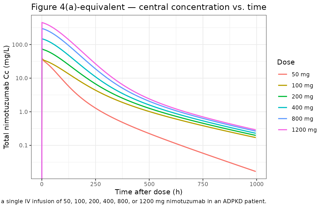

The simulated 50 mg curve shows the faster early decline visible in the published Figure 4A, providing visual support for the V₁ × (1 − 0.53) interpretation of the Table 2 row “V₁ change (D = 50 mg) [%] = 53” (see Errata section below for the rationale and remaining ambiguity).

ggplot(sim_typ_one, aes(time, peripheral1 / 9.92e-3, colour = dose_label)) +
  geom_line(linewidth = 0.8) +
  scale_y_log10() +
  labs(
    x = "Time after dose (h)",
    y = "Peripheral total nimotuzumab (mg/L)",
    colour = "Dose",
    title = "Figure 4(b)-equivalent — peripheral compartment",
    caption = "Replicates Figure 4(b) of Castro-Suárez 2020 (typical-value simulation)."
  ) +
  theme_bw()
#> Warning in scale_y_log10(): log-10 transformation introduced
#> infinite values.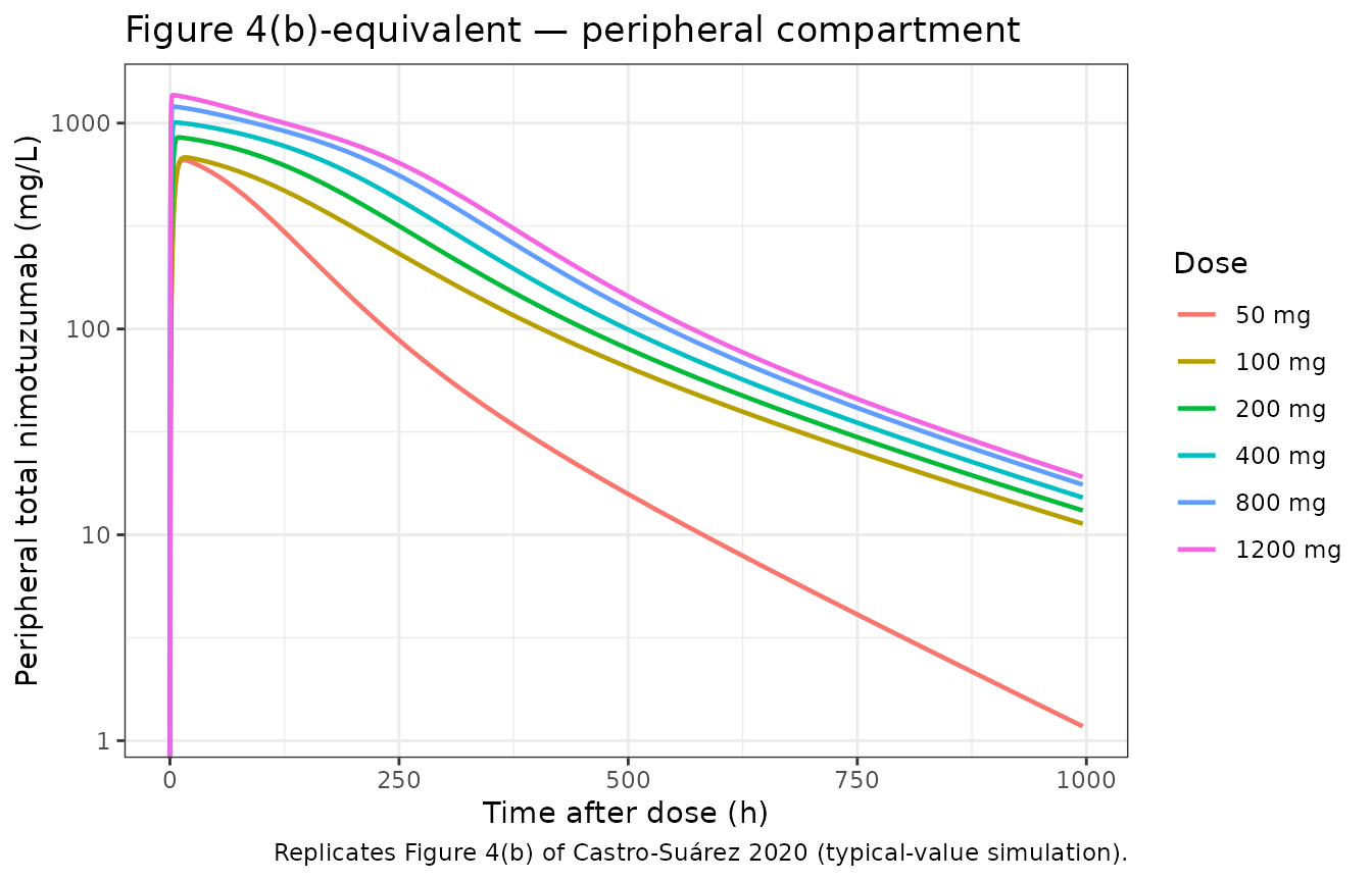

ggplot(sim_typ_one, aes(time, effect, colour = dose_label)) +
  geom_line(linewidth = 0.8) +
  geom_hline(yintercept = 1, linetype = "dashed", colour = "grey50") +
  labs(
    x = "Time after dose (h)",
    y = "Mediator level A3 (dimensionless; baseline = 1)",
    colour = "Dose",
    title = "Figure 4(c)-equivalent — mediator compartment",
    caption = "Replicates Figure 4(c) of Castro-Suárez 2020. Dashed line = baseline mediator level."
  ) +
  theme_bw()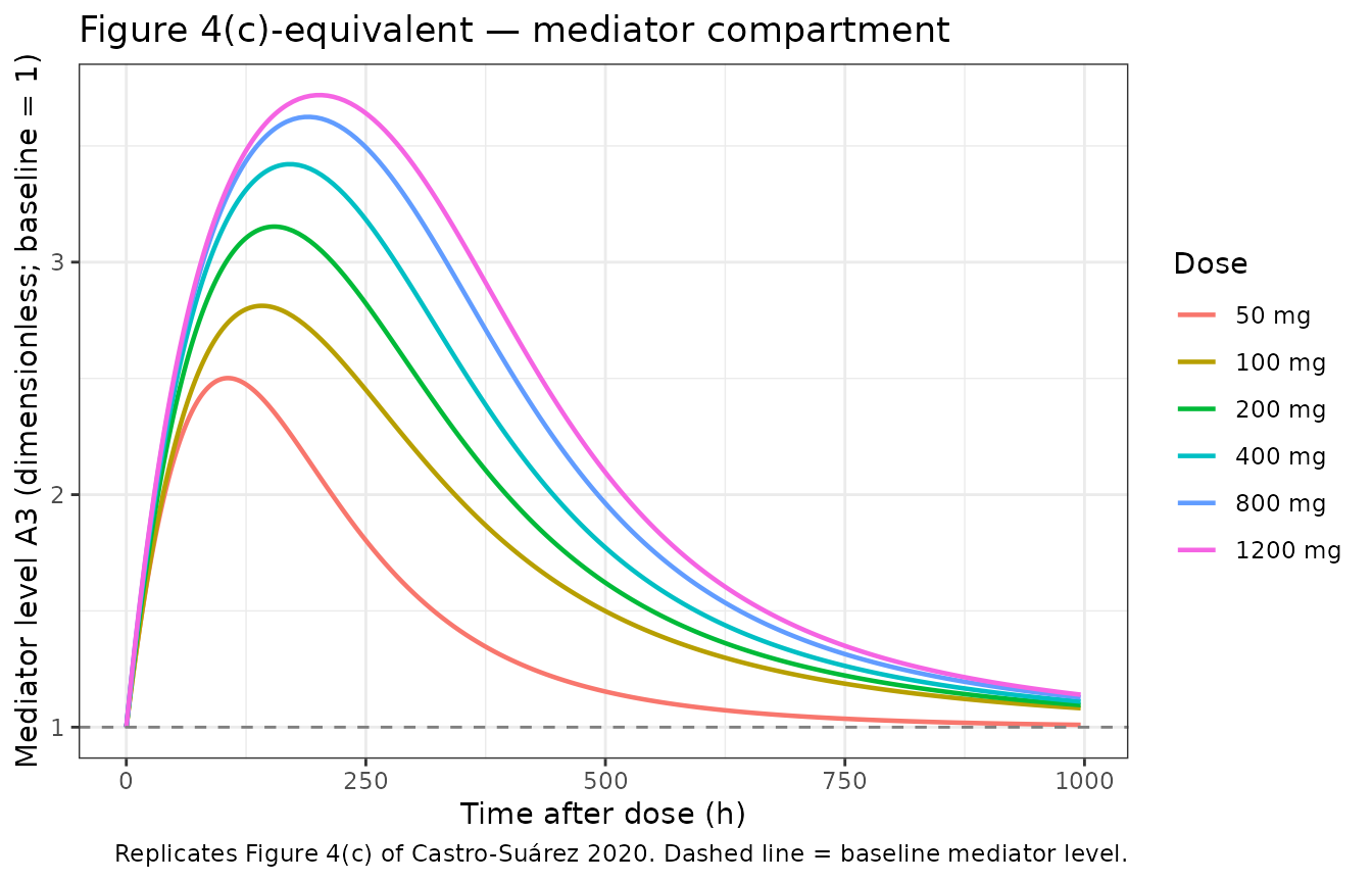

The dose-dependent mediator activation reproduces Castro-Suárez §3.3: maximum effect on the mediator approached at 100 mg (S₅₀ = 8.57 mg/L), with diminishing additional return at 200–1200 mg.

VPC-style cohort percentiles by dose

Stochastic simulation with the published η on R_totp and K_out produces a 50% prediction interval that narrows around the typical-value trajectory at high doses and broadens at the lowest 50 mg dose where the mediator sensitivity is highest.

vpc_summary <- sim_full |>
  filter(time <= 700, DOSE %in% c(50, 100, 200, 400)) |>
  group_by(DOSE, time) |>
  summarise(
    Q05 = stats::quantile(Cc, 0.05, na.rm = TRUE),
    Q50 = stats::quantile(Cc, 0.50, na.rm = TRUE),
    Q95 = stats::quantile(Cc, 0.95, na.rm = TRUE),
    .groups = "drop"
  ) |>
  mutate(dose_label = factor(paste(DOSE, "mg"), levels = paste(c(50, 100, 200, 400), "mg")))

ggplot(vpc_summary, aes(time, Q50, fill = dose_label, colour = dose_label)) +
  geom_ribbon(aes(ymin = Q05, ymax = Q95), alpha = 0.25, colour = NA) +
  geom_line(linewidth = 0.6) +
  scale_y_log10() +
  facet_wrap(~ dose_label, ncol = 2) +
  labs(
    x = "Time after dose (h)",
    y = "Total nimotuzumab Cc (mg/L)",
    title = "Stochastic-VPC — Cc vs. time by experimental dose group",
    caption = "Solid line = simulated median; ribbon = 5th–95th percentile of n = 100/dose virtual subjects."
  ) +
  theme_bw() +
  theme(legend.position = "none")
#> Warning in scale_y_log10(): log-10 transformation introduced infinite values.
#> log-10 transformation introduced infinite values.
#> log-10 transformation introduced infinite values.
#> log-10 transformation introduced infinite values.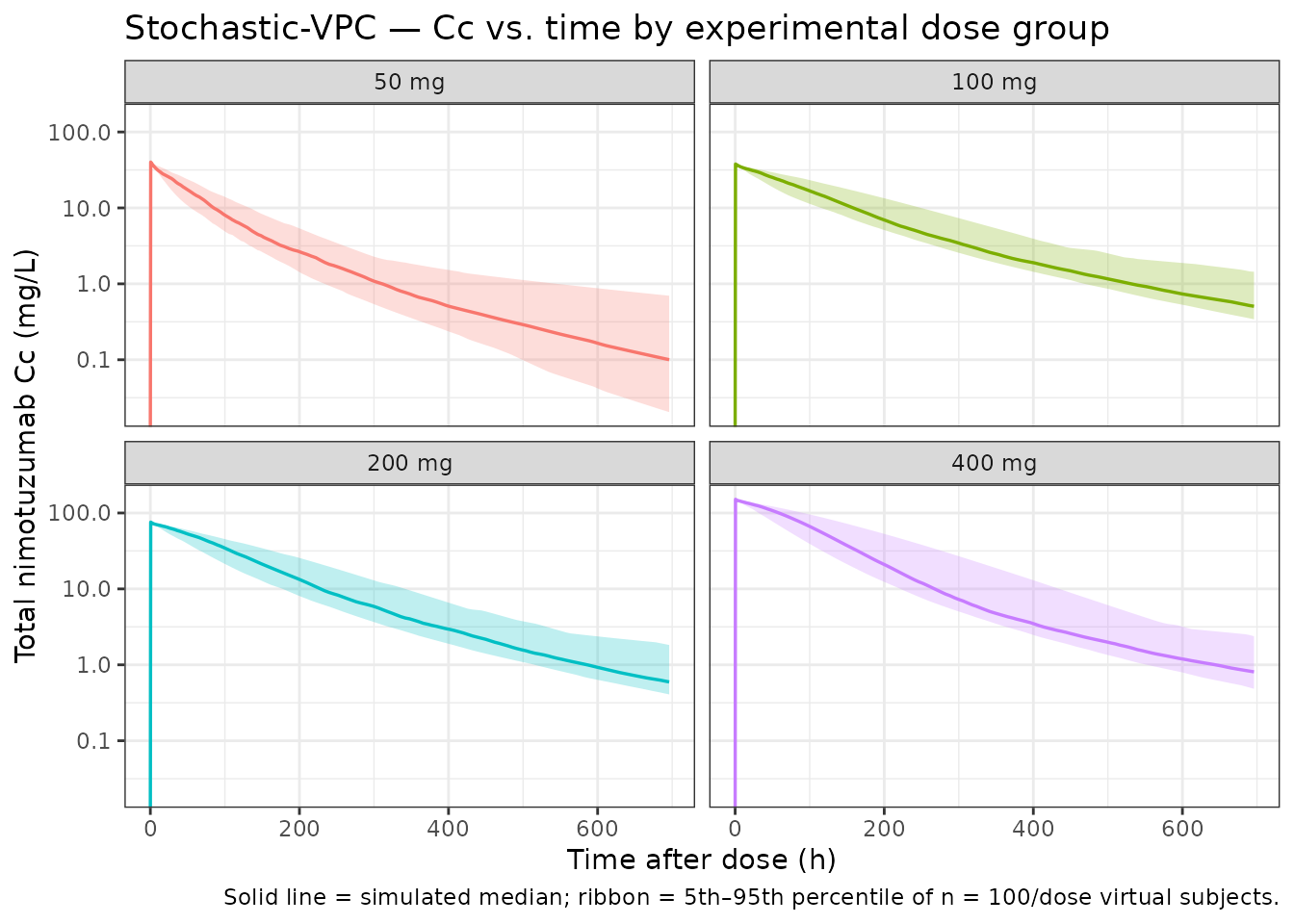

PKNCA validation

PKNCA Cmax / Tmax / AUC / half-life on the experimental dose range (50, 100, 200, 400 mg). The formula carries treatment as the dose-group grouping variable so the summary rolls up per cohort.

sim_nca <- sim_full |>
  filter(!is.na(Cc), DOSE %in% c(50, 100, 200, 400), time <= 700) |>
  transmute(
    id        = id,
    time      = time,
    Cc        = Cc,
    treatment = paste(DOSE, "mg")
  )

dose_nca <- d_sim |>
  filter(EVID == 1, DOSE %in% c(50, 100, 200, 400)) |>
  transmute(
    id        = id,
    time      = TIME,
    amt       = AMT,
    treatment = paste(DOSE, "mg")
  )

conc_obj <- PKNCA::PKNCAconc(sim_nca, Cc ~ time | treatment + id,
                             concu = "mg/L", timeu = "hour")
dose_obj <- PKNCA::PKNCAdose(dose_nca, amt ~ time | treatment + id,
                             doseu = "mg")

intervals <- data.frame(
  start       = 0,
  end         = Inf,
  cmax        = TRUE,
  tmax        = TRUE,
  aucinf.obs  = TRUE,
  half.life   = TRUE,
  clast.obs   = TRUE
)

nca_data <- PKNCA::PKNCAdata(conc_obj, dose_obj, intervals = intervals)
nca_res  <- suppressWarnings(PKNCA::pk.nca(nca_data))
#>  ■■                                 4% |  ETA:  1m
#>  ■■■■                               9% |  ETA:  1m
#>  ■■■■■                             14% |  ETA:  1m
#>  ■■■■■■                            18% |  ETA:  1m
#>  ■■■■■■■■                          23% |  ETA: 48s
#>  ■■■■■■■■■                         28% |  ETA: 45s
#>  ■■■■■■■■■■■                       32% |  ETA: 42s
#>  ■■■■■■■■■■■■                      37% |  ETA: 40s
#>  ■■■■■■■■■■■■■■                    42% |  ETA: 36s
#>  ■■■■■■■■■■■■■■■                   47% |  ETA: 33s
#>  ■■■■■■■■■■■■■■■■■                 52% |  ETA: 30s
#>  ■■■■■■■■■■■■■■■■■■                57% |  ETA: 27s
#>  ■■■■■■■■■■■■■■■■■■■■              62% |  ETA: 24s
#>  ■■■■■■■■■■■■■■■■■■■■■             67% |  ETA: 21s
#>  ■■■■■■■■■■■■■■■■■■■■■■■           72% |  ETA: 17s
#>  ■■■■■■■■■■■■■■■■■■■■■■■■          76% |  ETA: 15s
#>  ■■■■■■■■■■■■■■■■■■■■■■■■■         82% |  ETA: 11s
#>  ■■■■■■■■■■■■■■■■■■■■■■■■■■■       86% |  ETA:  8s
#>  ■■■■■■■■■■■■■■■■■■■■■■■■■■■■      91% |  ETA:  5s
#>  ■■■■■■■■■■■■■■■■■■■■■■■■■■■■■■    96% |  ETA:  2s

nca_tbl <- as.data.frame(nca_res$result) |>
  filter(PPTESTCD %in% c("cmax", "tmax", "aucinf.obs", "half.life", "clast.obs")) |>
  group_by(treatment, PPTESTCD) |>
  summarise(
    median = stats::median(PPORRES, na.rm = TRUE),
    p05    = stats::quantile(PPORRES, 0.05, na.rm = TRUE),
    p95    = stats::quantile(PPORRES, 0.95, na.rm = TRUE),
    .groups = "drop"
  ) |>
  mutate(treatment = factor(treatment, levels = c("50 mg", "100 mg", "200 mg", "400 mg"))) |>
  arrange(treatment, PPTESTCD)
nca_tbl
#> # A tibble: 20 × 5
#>    treatment PPTESTCD      median        p05       p95
#>    <fct>     <chr>          <dbl>      <dbl>     <dbl>
#>  1 50 mg     aucinf.obs  2867.     2193.      3803.   
#>  2 50 mg     clast.obs      0.100     0.0204     0.697
#>  3 50 mg     cmax          40.1      40.1       40.1  
#>  4 50 mg     half.life    130.       86.9      265.   
#>  5 50 mg     tmax           0.5       0.5        0.5  
#>  6 100 mg    aucinf.obs  4936.     4091.      6955.   
#>  7 100 mg    clast.obs      0.507     0.341      1.44 
#>  8 100 mg    cmax          37.9      37.9       37.9  
#>  9 100 mg    half.life    180.      130.       283.   
#> 10 100 mg    tmax           0.5       0.5        0.5  
#> 11 200 mg    aucinf.obs  9484.     7306.     13227.   
#> 12 200 mg    clast.obs      0.595     0.408      1.83 
#> 13 200 mg    cmax          75.8      75.8       75.8  
#> 14 200 mg    half.life    168.      115.       268.   
#> 15 200 mg    tmax           0.5       0.5        0.5  
#> 16 400 mg    aucinf.obs 17128.    12511.     26952.   
#> 17 400 mg    clast.obs      0.808     0.484      2.38 
#> 18 400 mg    cmax         152.      152.       152.   
#> 19 400 mg    half.life    165.      104.       255.   
#> 20 400 mg    tmax           0.5       0.5        0.5

Comparison against the published narrative values

Castro-Suárez 2020 does not publish a per-cohort NCA table; the comparison below uses the typical-patient values reported in Discussion §4 (V_ss = 2.64 L, V₁ = 2.63 L, V₂ = 9.92 × 10⁻³ L) and the model-informed dose-selection narrative (S₅₀ = 8.57 mg/L; maximum mediator activation reached at 100 mg).

# Vss is V1 + V2 from the model (typical-value trajectory).
vss_sim <- (sim_typ_one |> filter(DOSE == 100, time == 1000) |> nrow() > 0)  # sanity guard

vss_typical <- 2.63 + 9.92e-3

# Cmax for 100 mg (typical) — conc immediately at end of infusion (t = 0.5 h).
cmax_100mg_typ <- sim_typ_one |>
  filter(DOSE == 100, time == 0.5) |>
  pull(Cc)

# Cmax for 50 mg (typical) — sanity check on the V1 x (1 - 0.53) reduction for the
# 50 mg cohort (see Errata). With V1 = 2.63 * 0.47 = 1.2361 L, Cmax_typical ~=
# 50 / 1.2361 ~= 40.5 mg/L; without the reduction it would be 50 / 2.63 ~= 19 mg/L.
cmax_50mg_typ <- sim_typ_one |>
  filter(DOSE == 50, time == 0.5) |>
  pull(Cc)
cmax_50mg_no_v1shift <- 50 / 2.63

# Time above S50 = 8.57 mg/L for the typical 100 mg trajectory.
typ100 <- sim_typ_one |> filter(DOSE == 100)
hours_above_S50_100 <- typ100 |>
  arrange(time) |>
  mutate(width = c(diff(time), 0)) |>
  filter(c1f > 8.57) |>
  summarise(hours = sum(width)) |>
  pull(hours)

comparison <- tibble::tribble(
  ~metric,                                                 ~published,             ~simulated,                         ~units,
  "Vss (typical) = V1 + V2",                                2.64,                  vss_typical,                        "L",
  "Cmax @ 100 mg, end of 30-min infusion (typical)",        NA_real_,              cmax_100mg_typ,                     "mg/L",
  "Cmax @ 50 mg, end of 30-min infusion (typical)",         NA_real_,              cmax_50mg_typ,                      "mg/L",
  "Cmax @ 50 mg if V1 shift were not applied",              NA_real_,              cmax_50mg_no_v1shift,               "mg/L",
  "Free Cc above S50 (8.57 mg/L) duration @ 100 mg (typ.)", NA_real_,              hours_above_S50_100,                "h"
)
comparison
#> # A tibble: 5 × 4
#>   metric                                               published simulated units
#>   <chr>                                                    <dbl>     <dbl> <chr>
#> 1 Vss (typical) = V1 + V2                                   2.64      2.64 L    
#> 2 Cmax @ 100 mg, end of 30-min infusion (typical)          NA        37.9  mg/L 
#> 3 Cmax @ 50 mg, end of 30-min infusion (typical)           NA        40.1  mg/L 
#> 4 Cmax @ 50 mg if V1 shift were not applied                NA        19.0  mg/L 
#> 5 Free Cc above S50 (8.57 mg/L) duration @ 100 mg (ty…     NA       174.   h

The simulated typical-patient V_ss exactly matches the published 2.64 L (V₁ + V₂ are direct fixed-effect parameters; for doses other than 50 mg no covariate scaling applies). The typical Cmax at the 100-mg dose is approximately dose ÷ V₁ = 100 / 2.63 ≈ 38 mg/L immediately after infusion end, consistent with the y-axis of Figure 4(a). The typical Cmax at the 50-mg dose is approximately dose ÷ (V₁ × 0.47) = 50 / 1.236 ≈ 40 mg/L — i.e. higher than the un-adjusted 50 / 2.63 ≈ 19 mg/L value would be — which is what produces the faster early decline of the 50 mg curve in Figure 4A (smaller central volume → higher initial concentration and higher free-drug exposure that drives accelerated TMDD/mediator clearance). The simulated free-concentration window above S₅₀ = 8.57 mg/L provides the duration that the paper’s Discussion uses to argue that 100 mg is the maximum effective single dose.

Assumptions and deviations

Hill coefficient γ on the mediator sigmoid: fixed at 1. Equation (3) of Methods §2.3 includes a Hill coefficient γ on the sigmoid Emax of the mediator-synthesis term. γ is not listed in Table 2 (Final parameter estimates). The skill operator confirmed γ should be fixed at 1 because the parameter would have been listed if estimated, and the equation collapses to a hyperbolic Emax Smax · C / (S50 + C) when γ = 1. The packaged model writes the sigmoid in this hyperbolic form. If a future author correspondence indicates γ was estimated at a non-unit value, the model should be updated. Operator follow-up F8 in the upstream tracking notes records that the corresponding author has been emailed for confirmation.
No covariate effects. The covariate-search procedure (forward p < 0.05, backward p < 0.01) tested body weight, height, age, body surface area, creatinine clearance, serum creatinine, total kidney volume, total cyst volume, sex, and race; none was retained. The packaged covariateData is therefore an empty list. Body weight is carried in the virtual cohort dataset for realism (and so a future weight-stratified analysis remains expressible in user code) but does not enter any structural-parameter equation.
Total drug as the modeled state. The packaged model integrates total nimotuzumab amount (free + EGFR-bound) in each compartment and derives the free concentration via the closed-form QSS algebraic solution cfree = ½·(disc + √(disc² + 4·Kss·Ctotal)) where disc = Ctotal − R − Kss (Gibiansky et al. 2008). The paper integrates free amount with the dilution factor (1 + R·Kss/(Kss+Cf)²) in the denominator. The two parameterizations yield identical observable total nimotuzumab concentration Cc = Ctotal because the dilution factor is exactly dCtotal/dCfree under QSS.
Mediator compartment named effect. The paper labels the turnover state “A₃” or “mediator.” The packaged model uses the canonical nlmixr2lib compartment name effect (the registered indirect-response / turnover compartment, used identically by Ma_2020_sarilumab_anc.R). The mediator’s level multiplies the linear CL term in the central ODE.
Single-cohort study. The model is fit to one Cuban single-center phase I trial (n = 20, single-dose, four cohorts of 5 patients). Generalization to multiple-dose regimens, other indications (the paper contrasts with breast-cancer PK from a separate study), or pediatric / renal-impaired populations is not supported by the source data.
Below-LOQ data. All 422 observations were quantifiable; no BLQ handling is implemented.

Errata

V₁ change for the 50-mg dose cohort — direction inferred from Figure 4A, not stated in the paper text. Table 2 of Castro-Suárez 2020 lists a fixed-effect parameter V1 change (D = 50 mg) [%] with a final estimate of 53 %, bootstrap median 56, RSE 14 %, and bootstrap 95 % CI 43–69 %. The parameter is reported only as a Table 2 row: it is not described in Methods §2.3, in Results §3.2, in the Discussion, or in the V_ss footnote — all of which use the unmodified V₁ = 2.63 L. The direction of the adjustment (V₁ larger or smaller for the 50 mg cohort) is therefore not explicitly stated in the paper. This packaged model interprets the parameter as a 53 % decrease in V₁ for the 50 mg cohort (vc <- exp(lvc) * (1 - 0.53 * (DOSE == 50)); the published final model carries no IIV on V₁) on the basis of visual inspection of Figure 4A: the published 50 mg simulated central-compartment trajectory shows a faster early decline than the 100, 200, 400, 800, or 1200 mg trajectories, behavior consistent with a smaller central volume at 50 mg. This is documented as an Erratum-style ambiguity rather than a published correction; no erratum was located on PubMed, the MDPI landing page, or Google Scholar (search dates 2026-04-25). The corresponding author Víctor Mangas-Sanjuán (Universitat de València, victor.mangas@uv.es) has been contacted for confirmation of direction (operator follow-up F8 in the upstream tracking notes); if the author reply differs from the Figure-4A-based interpretation, this entry and the model file will be updated.

Reference

de Castro-Suarez N, Trame MN, Mangas-Sanjuan V, Garcia-Cremades M, Boix-Montanes A, Fernandez-Teruel C, Munoz-Camara A, Martin-Suarez A, Rebollo-Fernandez G, Lleonart-Vidal R. Semi-Mechanistic Pharmacokinetic Model to Guide the Dose Selection of Nimotuzumab in Patients with Autosomal Dominant Polycystic Kidney Disease. Pharmaceutics. 2020;12(12):1147. doi:10.3390/pharmaceutics12121147