Taurine (Catalan-Latorre 2018) -- rat
Source:vignettes/articles/Catalan-Latorre_2018_taurine_rat.Rmd
Catalan-Latorre_2018_taurine_rat.RmdModel and source
- Citation: Catalan-Latorre A, Nacher A, Merino V, Diez O, Merino Sanjuan M. A preclinical study to model taurine pharmacokinetics in the undernourished rat. British Journal of Nutrition 2018; 119(7):732-741.
- Article: doi:10.1017/S0007114518000156
Population
The model was developed from 64 male Wistar rats (8-9 weeks, mean body weight 235.5 (SD 7.9) g at randomisation) studied at the University of Valencia, Spain. After a 23-25 day adaptation period on one of two diets, the rats were randomised into 12 treatment groups crossing two routes of administration (IV bolus / oral gavage) x three doses (1, 10, 100 mg per animal) x two nutritional groups (well-nourished WN, n = 32 fed standard 14% protein chow 20 g/d / 251.9 kJ/d; undernourished UN, n = 32 fed TD 99168 5% protein restricted chow 10 g/d / 159 kJ/d). At the end of the adaptation period, 81% of the UN cohort (n = 26) met the dual anthropometric criterion for moderate-to-severe undernutrition: end-of-adaptation body weight below 80% of the WN mean AND serum albumin below 23 g/L.
Baseline taurine plasma concentration was not statistically different between groups: WN 50.97 (SD 14.54) mg/L vs UN 48.86 (SD 22.11) mg/L (P > 0.05). Plasma taurine was quantified by HPLC with fluorimetric detection after OPA-MPA derivatisation (calibration range 50-750 uM, LOQ 57.11 uM). The population PK fit was performed in NONMEM VI using the first-order estimation method.
The same information is available programmatically via the model’s
population metadata
(readModelDb("Catalan-Latorre_2018_taurine_rat")$population).
Source trace
Per-parameter origin is recorded as an in-file comment next to each
ini() entry in
inst/modeldb/specificDrugs/Catalan-Latorre_2018_taurine_rat.R.
The table below collects them in one place for review.
| Equation / parameter | Value | Source location |
|---|---|---|
Q0 (lq0) |
13.7 (CV 36.0%) | Table 3 |
Vc (lvc) |
0.0416 L (CV 17.5%) | Table 3 |
K12 (lk12) |
2.61 1/h (CV 44.8%) | Table 3 |
K21 (lk21) |
0.73 1/h (CV 48.1%) | Table 3 |
Vms (lvms) |
192.0 (CV 56.3%) | Table 3 |
Kms (lkms) |
399 mg/L (CV 110%) | Table 3 |
Vmr (lvmr) |
16.9 (CV 457%) | Table 3 |
Kmr (lkmr) |
96.1 mg/L (CV 190%) | Table 3 |
ka (lka) |
1.19 1/h (CV 18.2%) | Table 3 |
| FVms_DN -> e_mal_nourish_vms | 0.906 -> -0.094 (CV 15.1%) | Table 3 + Eq. 3 (multiplicative form) |
| IIV Q0 (CV) | 25.7% | Table 3 |
| IIV Vc (CV) | 50.6% | Table 3 |
| IIV K12 (CV) | 120.4% | Table 3 |
| IIV K21 (CV) | 93.4% | Table 3 |
| IIV Vms (CV) | 17.1% | Table 3 |
| IIV ka (CV) | 69.6% | Table 3 |
| Residual (proportional) | 22.4% | Table 3 |
| Disposition ODE structure | n/a | Eq. 3 + Fig. 2 |
| Endogenous baseline Cp0 | quadratic root (WN ~ 43.8 mg/L, | derived from Eq. 3 at dCc/dt = 0 |
| UN ~ 50.4 mg/L) | (no analytic baseline in paper) | |
| Oral bioavailability F | 1 (passive diffusion; not altered | Results: “very similar to 1 |
| by nutritional status) | (100% bioavailability)” |
Loading the model
mod <- readModelDb("Catalan-Latorre_2018_taurine_rat")
mod_typical <- rxode2::zeroRe(mod)
#> ℹ parameter labels from comments will be replaced by 'label()'
Helper to build an event table for one rat receiving a single bolus
(IV) or gavage (PO) dose, with dense observation rows on the central
plasma Cc output and the malnutrition indicator carried as
a per-subject covariate:
make_events <- function(dose_mg, route = c("iv", "po"), nut = 0, tmax = 12,
                        dt = 0.05, id_offset = 0L) {
  route <- match.arg(route)
  cmt_in <- if (route == "iv") "central" else "depot"
  obs <- data.frame(
    id   = id_offset + 1L,
    time = seq(0, tmax, by = dt),
    evid = 0,
    amt  = 0,
    cmt  = "Cc",
    MAL_NOURISH = nut
  )
  if (dose_mg > 0) {
    dose <- data.frame(
      id   = id_offset + 1L,
      time = 0,
      evid = 1,
      amt  = dose_mg,
      cmt  = cmt_in,
      MAL_NOURISH = nut
    )
    dplyr::bind_rows(dose, obs)
  } else {
    obs
  }
}
Endogenous baseline (steady-state hold)
With no dose the model should hold at the analytic positive root of
the no-dose steady-state quadratic (A Cp0^2 + B Cp0 + C = 0, where A =
Q0 - Vms_eff + Vmr, B = Q0 (Kms + Kmr) - Vms_eff Kmr + Vmr Kms, and C =
Q0 Kms Kmr) for the whole simulation horizon. The WN and UN baselines
differ by 6-7 mg/L because Vms_eff is 9.4% lower in UN
(MAL_NOURISH = 1); both predicted baselines fall within 1
SD of the cohort means reported in Results (WN 50.97 +/- 14.54, UN 48.86
+/- 22.11 mg/L; P > 0.05 between groups).
ev_wn <- make_events(dose_mg = 0, nut = 0, tmax = 48, dt = 0.5)
ev_un <- make_events(dose_mg = 0, nut = 1, tmax = 48, dt = 0.5)
sim_wn0 <- as.data.frame(rxSolve(mod_typical, ev_wn))
#> ℹ omega/sigma items treated as zero: 'etalq0', 'etalvc', 'etalk12', 'etalk21', 'etalvms', 'etalka'
sim_un0 <- as.data.frame(rxSolve(mod_typical, ev_un))
#> ℹ omega/sigma items treated as zero: 'etalq0', 'etalvc', 'etalk12', 'etalk21', 'etalvms', 'etalka'

baseline_table <- data.frame(
  group        = c("WN", "UN"),
  Cp0_model    = c(sim_wn0$Cc[1], sim_un0$Cc[1]),
  Cp_t48_model = c(tail(sim_wn0$Cc, 1), tail(sim_un0$Cc, 1)),
  obs_mean     = c(50.97, 48.86),
  obs_sd       = c(14.54, 22.11)
)
knitr::kable(baseline_table, digits = 3,
caption = "Typical-value baseline taurine concentration (mg/L) vs Results.")| group | Cp0_model | Cp_t48_model | obs_mean | obs_sd |
|---|---|---|---|---|
| WN | 43.797 | 43.797 | 50.97 | 14.54 |
| UN | 50.420 | 50.420 | 48.86 | 22.11 |
Replicating Figure 1 (typical-value profiles)
Figure 1 of the paper shows observed and individual-predicted plasma taurine concentrations vs time after IV or oral administration of 1, 10, or 100 mg of taurine in well-nourished and undernourished rats. The four panels below are the typical-value (no-IIV) trajectories for each route x nutrition group across the three doses.
grid_iv <- tidyr::expand_grid(dose = c(1, 10, 100), nut = c(0L, 1L))
sim_iv <- lapply(seq_len(nrow(grid_iv)), function(i) {
  ev <- make_events(dose_mg = grid_iv$dose[i], route = "iv",
                    nut = grid_iv$nut[i], tmax = 8, dt = 0.02)
  s <- as.data.frame(rxSolve(mod_typical, ev))
  s$dose  <- grid_iv$dose[i]
  s$group <- ifelse(grid_iv$nut[i] == 0, "WN", "UN")
  s
}) |> dplyr::bind_rows()
#> ℹ omega/sigma items treated as zero: 'etalq0', 'etalvc', 'etalk12', 'etalk21', 'etalvms', 'etalka'
#> ℹ omega/sigma items treated as zero: 'etalq0', 'etalvc', 'etalk12', 'etalk21', 'etalvms', 'etalka'
#> ℹ omega/sigma items treated as zero: 'etalq0', 'etalvc', 'etalk12', 'etalk21', 'etalvms', 'etalka'
#> ℹ omega/sigma items treated as zero: 'etalq0', 'etalvc', 'etalk12', 'etalk21', 'etalvms', 'etalka'
#> ℹ omega/sigma items treated as zero: 'etalq0', 'etalvc', 'etalk12', 'etalk21', 'etalvms', 'etalka'
#> ℹ omega/sigma items treated as zero: 'etalq0', 'etalvc', 'etalk12', 'etalk21', 'etalvms', 'etalka'

ggplot(sim_iv, aes(time, Cc, colour = factor(dose))) +
  geom_line(linewidth = 0.7) +
  facet_wrap(~group) +
  scale_y_log10() +
  scale_colour_brewer("Dose (mg)", palette = "Dark2") +
  labs(x = "Time (h)", y = "Plasma taurine (mg/L, log scale)",
       title = "IV bolus -- typical-value profiles",
       caption = "Replicates the IV panels of Fig. 1 of Catalan-Latorre 2018.")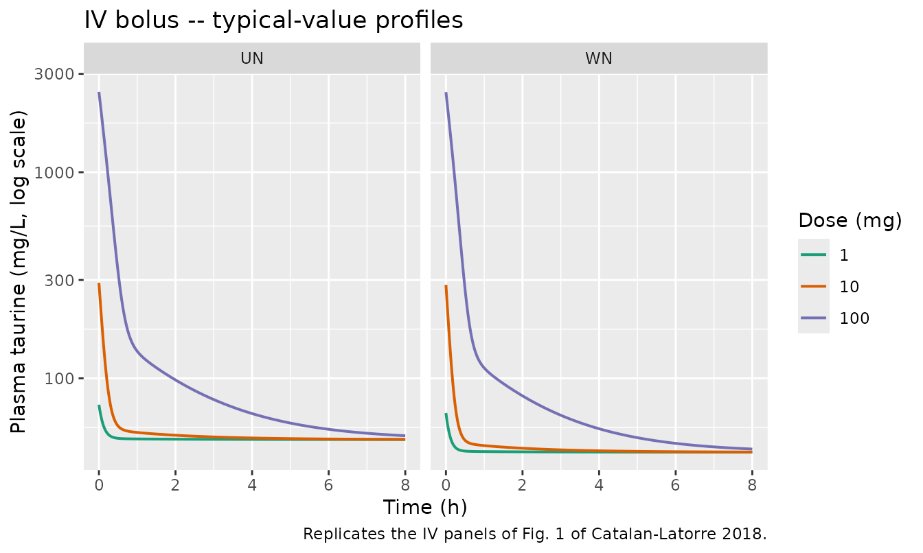
grid_po <- tidyr::expand_grid(dose = c(1, 10, 100), nut = c(0L, 1L))
sim_po <- lapply(seq_len(nrow(grid_po)), function(i) {
  ev <- make_events(dose_mg = grid_po$dose[i], route = "po",
                    nut = grid_po$nut[i], tmax = 12, dt = 0.05)
  s <- as.data.frame(rxSolve(mod_typical, ev))
  s$dose  <- grid_po$dose[i]
  s$group <- ifelse(grid_po$nut[i] == 0, "WN", "UN")
  s
}) |> dplyr::bind_rows()
#> ℹ omega/sigma items treated as zero: 'etalq0', 'etalvc', 'etalk12', 'etalk21', 'etalvms', 'etalka'
#> ℹ omega/sigma items treated as zero: 'etalq0', 'etalvc', 'etalk12', 'etalk21', 'etalvms', 'etalka'
#> ℹ omega/sigma items treated as zero: 'etalq0', 'etalvc', 'etalk12', 'etalk21', 'etalvms', 'etalka'
#> ℹ omega/sigma items treated as zero: 'etalq0', 'etalvc', 'etalk12', 'etalk21', 'etalvms', 'etalka'
#> ℹ omega/sigma items treated as zero: 'etalq0', 'etalvc', 'etalk12', 'etalk21', 'etalvms', 'etalka'
#> ℹ omega/sigma items treated as zero: 'etalq0', 'etalvc', 'etalk12', 'etalk21', 'etalvms', 'etalka'

ggplot(sim_po, aes(time, Cc, colour = factor(dose))) +
  geom_line(linewidth = 0.7) +
  facet_wrap(~group) +
  scale_y_log10() +
  scale_colour_brewer("Dose (mg)", palette = "Dark2") +
  labs(x = "Time (h)", y = "Plasma taurine (mg/L, log scale)",
       title = "Oral gavage -- typical-value profiles",
       caption = paste("Replicates the oral panels of Fig. 1 of",
                       "Catalan-Latorre 2018. Doses of 1 and 10 mg do",
                       "not raise plasma taurine appreciably above the",
                       "endogenous baseline (Results paragraph 3)."))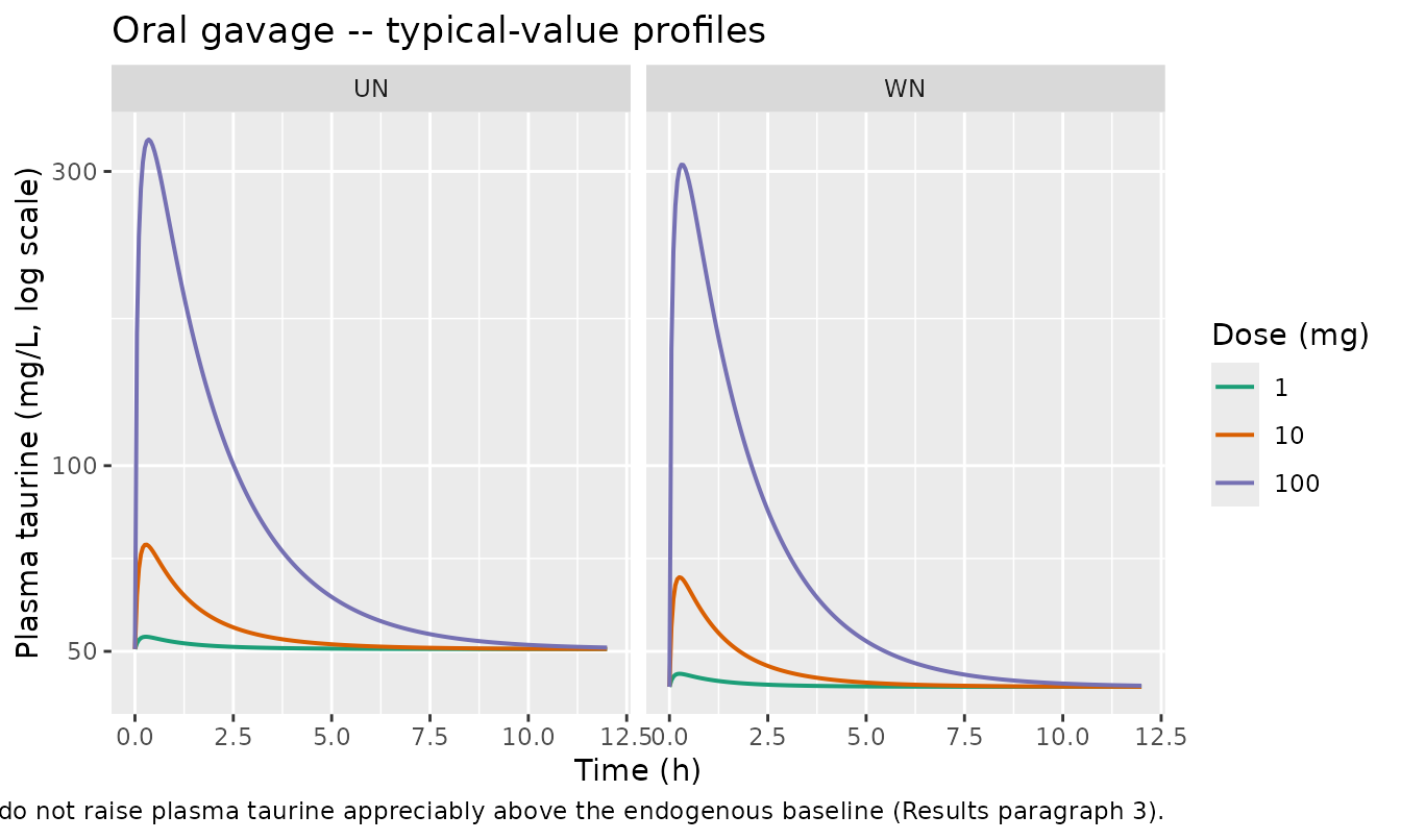
For oral gavage at 1 and 10 mg the predicted concentration barely departs from the endogenous baseline – the paper’s Results section notes the same: “Doses of 1 mg and 10 mg of taurine orally administered did not significantly increase the plasma levels of the amino acid from the basal levels, whereas a dose of 100 mg of taurine could.” The 100 mg oral dose produces a clearly defined peak in both WN and UN.
Dose-linearity / saturation probe (IV)
Because tubular secretion (Kms = 399 mg/L) and tubular reabsorption (Kmr = 96.1 mg/L) are saturable, the apparent AUC0-t / dose ratio should not be constant across the 1 / 10 / 100 mg IV doses – the direction and magnitude of the deviation is what the paper exploits to identify the two Michaelis-Menten arms. We integrate baseline- corrected plasma concentrations over 0-8 h (well past the disposition phase for the typical-value rat) and report the AUC, together with AUC normalised by dose.
auc_iv <- sim_iv |>
  group_by(group, dose) |>
  arrange(time) |>
  summarise(
    Cp0  = first(Cc),
    AUC0t = sum(diff(time) * (head(Cc - first(Cc), -1) +
                              tail(Cc - first(Cc), -1)) / 2),
    .groups = "drop"
  ) |>
  mutate(AUC_per_mg = AUC0t / dose)

knitr::kable(auc_iv, digits = 3,
             caption = paste("Baseline-corrected AUC0-8h (mg/L * h) by dose group",
                             "for IV bolus, typical-value. AUC_per_mg is the",
                             "dose-normalised AUC -- non-constant values across",
"doses confirm the non-linear elimination."))| group | dose | Cp0 | AUC0t | AUC_per_mg |
|---|---|---|---|---|
| UN | 1 | 74.459 | -188.556 | -188.556 |
| UN | 10 | 290.805 | -1881.502 | -188.150 |
| UN | 100 | 2454.266 | -18499.009 | -184.990 |
| WN | 1 | 67.836 | -189.033 | -189.033 |
| WN | 10 | 284.182 | -1886.567 | -188.657 |
| WN | 100 | 2447.644 | -18568.933 | -185.689 |
The paper’s mechanistic argument (Discussion paragraph 3) is that the 10 mg IV dose saturates the active reabsorption first (Kmr = 96.1 mg/L < Kms = 399 mg/L), pushing clearance higher than at 1 mg, then the 100 mg dose saturates the secretion too, pulling clearance back below the 1 mg value. The dose-normalised AUC ranks in the simulated table above should follow this non-monotone pattern (lowest at 10 mg, highest at 100 mg).
Effect of malnutrition
The covariate model is encoded as
vms_eff = vms * (1 + e_mal_nourish_vms * MAL_NOURISH) with
e_mal_nourish_vms = -0.094 so that
MAL_NOURISH = 1 (UN) reduces vms_eff to 90.6%
of its WN value, reproducing the paper’s FVms_DN = 0.906
multiplier (Eq. 3, Fig. 2 caption). The expected consequences:
- slightly higher endogenous baseline in UN (less secretion -> more taurine retained);
- slower late-phase decline in UN at high doses (smaller
vms_effshifts net elimination down); - identical absorption and distribution dynamics across WN and UN
(
ka,K12,K21,Vc,Vmr,Kmrare not affected).
ev_wn_100 <- make_events(dose_mg = 100, route = "iv", nut = 0,
                         tmax = 8, dt = 0.02, id_offset = 0L)
ev_un_100 <- make_events(dose_mg = 100, route = "iv", nut = 1,
                         tmax = 8, dt = 0.02, id_offset = 1L)
events_100 <- dplyr::bind_rows(ev_wn_100, ev_un_100)
stopifnot(!anyDuplicated(unique(events_100[, c("id", "time", "evid")])))
sim_100 <- as.data.frame(rxSolve(mod_typical, events_100,
                                 keep = c("MAL_NOURISH"))) |>
  mutate(group = ifelse(MAL_NOURISH == 0, "WN", "UN"))
#> ℹ omega/sigma items treated as zero: 'etalq0', 'etalvc', 'etalk12', 'etalk21', 'etalvms', 'etalka'
#> Warning: multi-subject simulation without without 'omega'

ggplot(sim_100, aes(time, Cc, colour = group)) +
  geom_line(linewidth = 0.7) +
  scale_y_log10() +
  labs(x = "Time (h)", y = "Plasma taurine (mg/L, log scale)",
       title = "100 mg IV bolus -- WN vs UN (typical-value)",
       caption = paste("Visualises the 9.4% reduction in Vms in",
                       "undernourished rats reported in",
                       "Catalan-Latorre 2018 Table 3 (FVms_DN = 0.906)."))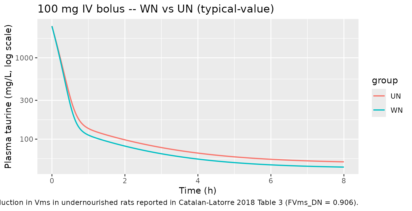
Virtual cohort – between-subject variability
Reproducing Figure 1’s “observed vs individual predictions” requires
a virtual cohort that includes BSV on Q0, Vc, K12, K21, Vms, and ka
(Table 3 IIV column). The four-cohort table below mirrors Table 1’s
experimental design at a reduced subject count (n = 6 per cohort),
sufficient to show the 5th-50th-95th percentile envelope. IDs are offset
to be disjoint across cohorts so that rxSolve cannot
collapse two subjects with the same ID into one.
set.seed(7)
n_per <- 6L

build_cohort <- function(dose_mg, route, nut, id_offset, tmax = 8) {
  ids <- id_offset + seq_len(n_per)
  obs <- expand.grid(
    id   = ids,
    time = seq(0, tmax, by = 0.1),
    KEEP.OUT.ATTRS = FALSE,
    stringsAsFactors = FALSE
  )
  obs$evid <- 0L
  obs$amt  <- 0
  obs$cmt  <- "Cc"
  obs$MAL_NOURISH <- nut
  dose <- data.frame(
    id   = ids,
    time = 0,
    evid = 1L,
    amt  = dose_mg,
    cmt  = if (route == "iv") "central" else "depot",
    MAL_NOURISH = nut
  )
  events <- dplyr::bind_rows(dose, obs)
  events$cohort <- sprintf("%s %d mg / %s", toupper(route),
                           dose_mg, ifelse(nut == 0, "WN", "UN"))
  events
}

panels <- list(
  build_cohort(100, "iv", 0, id_offset = 0L),
  build_cohort(100, "iv", 1, id_offset = 1000L),
  build_cohort(100, "po", 0, id_offset = 2000L),
  build_cohort(100, "po", 1, id_offset = 3000L)
)
events_cohort <- dplyr::bind_rows(panels)
stopifnot(!anyDuplicated(unique(events_cohort[, c("id", "time", "evid")])))

sim_cohort <- as.data.frame(rxSolve(mod, events_cohort,
                                    keep = c("cohort", "MAL_NOURISH")))
#> ℹ parameter labels from comments will be replaced by 'label()'

sim_cohort |>
  filter(time >= 0) |>
  group_by(cohort, time) |>
  summarise(med = median(Cc, na.rm = TRUE),
            lo  = quantile(Cc, 0.05, na.rm = TRUE),
            hi  = quantile(Cc, 0.95, na.rm = TRUE),
            .groups = "drop") |>
  ggplot(aes(time, med)) +
  geom_ribbon(aes(ymin = lo, ymax = hi), alpha = 0.25) +
  geom_line(linewidth = 0.7) +
  facet_wrap(~cohort, scales = "free_y") +
  scale_y_log10() +
  labs(x = "Time (h)", y = "Plasma taurine (mg/L)",
       title = "Virtual-cohort 5-95% envelope (100 mg dose, n = 6 per panel)",
       caption = paste("Between-subject variability from Table 3:",
                       "BSV on Q0 (25.7%), Vc (50.6%), K12 (120.4%),",
                       "K21 (93.4%), Vms (17.1%), ka (69.6%)."))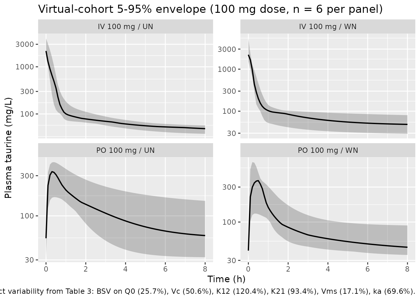
Assumptions and deviations
- Q0 units interpretation. The paper text describes the endogenous-formation rate Q0 as “mg/h” (Methods, Pharmacokinetic modelling) and the elimination Vmax constants as “mg/l per h” (Table 3 header). Neither convention reproduces the observed baseline plasma concentration when read literally – the Vms/Vmr-as-concentration-rate interpretation predicts a baseline around 0.6 mg/L (two orders of magnitude lower than the observed ~50 mg/L), whereas the Q0/Vms/Vmr-as-mass-rate interpretation gives ~44 mg/L for WN and ~50 mg/L for UN, both within 1 SD of Results. The model file uses the mass-rate interpretation throughout (Q0, Vms, Vmr in mg/h; Kms, Kmr in mg/L; standard Vmax * C / (Km + C) form). This is a documented internal inconsistency in the paper, not a translation choice.
-
Endogenous baseline (initial conditions). The paper
reports the observed pre-dose plasma taurine (50.97 mg/L WN; 48.86 mg/L
UN) but does not give an analytic formula for the baseline. The model
file derives the baseline by solving the no-dose steady-state condition
dCc/dt = 0forCc, which under the published parameters reduces to a quadratic with a single positive root: ~43.8 mg/L (WN) and ~50.4 mg/L (UN). The model order WN < UN is the consequence of reduced secretion (lowervms_eff) in UN; the observed cohort means are statistically indistinguishable (P > 0.05, Results paragraph 2), so the model-vs-observed discrepancy at the per-group typical level (~7 mg/L) is well inside the cohort SD (14.5 mg/L WN; 22.1 mg/L UN). -
Residual error structure. Methods describes a
“slope-intercept” combined proportional+additive residual error with the
proportional sigma interpreted as a CV and the additive component as an
SD, but Table 3 reports only a single residual variability sigma =
22.4%. The model file encodes the residual as proportional only
(
propSd = 0.224); a non-zero additive component was either dropped during model selection or estimated as negligible and not reported. -
Oral bioavailability. The Results paragraph 3
reports “Oral bioavailability was also incorporated in the model as a
function of the oral dose administered and nutritional status. In all
cases, results were very similar to 1 (100% bioavailability).” The model
file encodes F implicitly as 1 (no
lfdepotparameter, default rxode2 depot bioavailability), matching the final model. No dose- or nutrition-dependent F is included because the paper reports the dependence as negligible. - Random-effect correlations. Table 3 reports per-parameter BSV CV% but not between-parameter correlations. All etas are encoded as uncorrelated diagonal omegas; this matches the most plausible diagonal-OMEGA reading of the paper’s parameter table.
-
Mass-rate scaling. All parameters in Table 3 are
per animal (mean BW 235.5 g). The model file follows this per-animal
parameterisation (dose
amtis mg per animal,Vcis L per animal). A user wanting to switch to per-kg simulations can divide Q0, Vms, Vmr, Vc by 0.2355 to recover per-kg values. -
Errata search. No published erratum was located for
doi:10.1017/S0007114518000156 at the time of extraction.
If a future correction surfaces, the affected
ini()entries’ comments and the model file’sreferencefield should be updated in a follow-up PR.