Metoprolol (Eugene 2016)
Source:vignettes/articles/Eugene_2016_metoprolol.Rmd
Eugene_2016_metoprolol.RmdModel and source
- Citation: Eugene AR. Gender based Dosing of Metoprolol in the Elderly using Population Pharmacokinetic Modeling and Simulations. Int J Clin Pharmacol Toxicol. 2016;5(3):209-215. doi:10.19070/2167-910X-1600035
- Description: One-compartment population PK model for oral metoprolol tartrate with first-order absorption and lag time in elderly inpatients with multiple comorbidities; sex as the only covariate on apparent clearance (Eugene 2016).
- Article: Int J Clin Pharmacol Toxicol 2016;5(3):209-215 (open access)
Population
Eugene 2016 fit a one-compartment population PK model to digitized concentration-time data from seven of the ten chronically ill elderly inpatients enrolled in the Lundborg & Steen 1976 study at the University of Goteborg in Sweden. The retained cohort comprised 3 females (age 83 +/- 13 years, weight 58 +/- 13 kg) and 4 males (age 65 +/- 6 years, weight 65 +/- 6 kg); each subject received a single 50 mg oral metoprolol tartrate tablet with 100 mL water after a minimum 10-hour overnight fast. Body weight was tested as a covariate on the absorption rate constant Ka, apparent clearance CL/F, apparent volume V/F, and lag time Tlag, but its inclusion increased the AIC and reduced biological plausibility, so it was excluded from the final model (Eugene 2016 Discussion paragraph 1). Sex on apparent clearance was the only covariate retained in the final model.
The same information is available programmatically via
readModelDb("Eugene_2016_metoprolol")$population.
Source trace
Per-parameter origin is recorded as an in-file comment next to each
ini() entry in
inst/modeldb/specificDrugs/Eugene_2016_metoprolol.R. The
table below collects them for review.
| Equation / parameter | Value | Source location |
|---|---|---|
| Structure | One-compartment, first-order absorption with lag time, first-order elimination | Eugene 2016 Results page 211: “a one-compartment model with first-order elimination and first-order absorption was chosen”; matches the prior Kaila 2007 metoprolol popPK structure. |
llag (lag time) |
log(0.469) h |
Eugene 2016 Table 1, row “Tlag (hr): Lag Time”, estimate = 0.469 (RSE 4%). |
lka (absorption) |
log(0.235) 1/h |
Eugene 2016 Table 1, row “Ka (hr^-1): Absorption Rate Constant”, estimate = 0.235 (RSE 8%). |
lvc (apparent Vc/F) |
log(38) L |
Eugene 2016 Table 1, row “V (L): Volume of Distribution”, estimate = 38 (RSE 95%). |
lcl (female-ref CL/F) |
log(59.1) L/h |
Eugene 2016 Table 1, row “CL Females (L/hr): Apparent Female Clearance”, estimate = 59.1 (RSE 12%); the female value is the structural reference of the MONOLIX model. |
e_sexf_cl (male effect on CL) |
0.572 |
Eugene 2016 Table 1, row “betaCL Male (%): increase in clearance rate in males”, estimate = 0.572 (RSE 24%, p = 2.70e-5). CL_Male = CL_Female * exp(0.572) = 105 L/h (paper’s reported male CL, Table 1 row “CL Males”). |
etallag IIV |
0.030 |
Eugene 2016 Table 1, row “omega_Tlag, variance for Tlag”, omega^2 = 0.030 (RSE 113%; reported CV ~17%). |
etalka IIV |
0.052 |
Eugene 2016 Table 1, row “omega_Ka, variance for Ka”, omega^2 = 0.052 (RSE 254%; reported CV ~23%). |
etalvc IIV |
2.43 |
Eugene 2016 Table 1, row “omega_V, variance for V”, omega^2 = 2.43 (RSE 27%; reported CV ~155%). |
etalcl IIV |
0.143 |
Eugene 2016 Table 1, row “omega_CL, variance for CL”, omega^2 = 0.143 (RSE 39%; reported CV ~38%). |
addSd residual |
12.2 ng/mL |
Eugene 2016 Table 1, row “sigma (ng/mL): Residual (intra-individual) concentration”, estimate = 12.2 (RSE 10%). Additive on the linear concentration scale. |
| Unit conversion | Cc <- 1000 * central / vc |
Doses in mg and volumes in L give central / vc in mg/L;
the paper reports concentrations in ng/mL (1 mg/L = 1000 ng/mL), so the
model multiplies by 1000 to align with the paper’s reported sigma
units. |
Virtual cohort
Original observed concentration-time profiles were digitized by Eugene 2016 from Lundborg & Steen 1976 and are not redistributed here. The cohort below approximates the Eugene 2016 Table 1 demographics: 3 females / 4 males with the reported per-sex weight means and SDs, expanded to 250 virtual subjects per sex to give a well-resolved median + 90% percentile envelope. Each subject receives a single 50 mg oral metoprolol tartrate dose, matching the Lundborg 1976 protocol.
set.seed(20160519) # publication date 2016-05-19

n_per_sex <- 250L

make_cohort <- function(n, SEXF, wt_mean, wt_sd, id_offset = 0L) {
  label <- if (SEXF == 1L) "Female (50 mg)" else "Male (50 mg)"
  tibble(
    id        = id_offset + seq_len(n),
    SEXF      = as.integer(SEXF),
    WT        = pmin(pmax(rnorm(n, mean = wt_mean, sd = wt_sd), 45), 80),
    treatment = factor(label, levels = c("Male (50 mg)", "Female (50 mg)"))
  )
}

cohort <- bind_rows(
  make_cohort(n = n_per_sex, SEXF = 0L, wt_mean = 65, wt_sd = 6,  id_offset = 0L),
  make_cohort(n = n_per_sex, SEXF = 1L, wt_mean = 58, wt_sd = 13, id_offset = n_per_sex)
)

obs_times <- sort(unique(c(
  seq(0,    3, by = 0.1),   # dense across the absorption phase / Cmax
  seq(3.5, 12, by = 0.5),
  seq(13,  24, by = 1)
)))

dose_rows <- cohort |>
  mutate(time = 0, amt = 50, cmt = "depot", evid = 1L)

obs_rows <- cohort |>
  tidyr::crossing(time = obs_times) |>
  mutate(amt = 0, cmt = NA_character_, evid = 0L)

events <- bind_rows(dose_rows, obs_rows) |>
  select(id, time, amt, cmt, evid, SEXF, WT, treatment) |>
  arrange(id, time, desc(evid))

stopifnot(!anyDuplicated(unique(events[, c("id", "time", "evid")])))
Simulation
mod <- rxode2::rxode2(readModelDb("Eugene_2016_metoprolol"))
#> ℹ parameter labels from comments will be replaced by 'label()'
sim <- rxode2::rxSolve(mod, events = events, keep = c("SEXF", "WT", "treatment"))
Deterministic typical-value (no IIV) simulation for the published-Table 2 comparison below:
mod_typ <- mod |> rxode2::zeroRe()

typ_cohort <- tibble(
  id        = 1:2,
  SEXF      = c(0L, 1L),
  WT        = c(65, 58),
  treatment = factor(c("Male (50 mg)", "Female (50 mg)"),
                     levels = c("Male (50 mg)", "Female (50 mg)"))
)

typ_doses <- typ_cohort |> mutate(time = 0, amt = 50, cmt = "depot", evid = 1L)
typ_obs   <- typ_cohort |> tidyr::crossing(time = obs_times) |>
  mutate(amt = 0, cmt = NA_character_, evid = 0L)

typ_events <- bind_rows(typ_doses, typ_obs) |>
  select(id, time, amt, cmt, evid, SEXF, WT, treatment) |>
  arrange(id, time, desc(evid))

sim_typ <- rxode2::rxSolve(mod_typ, events = typ_events,
                           keep = c("SEXF", "WT", "treatment"))
#> ℹ omega/sigma items treated as zero: 'etaltlag', 'etalka', 'etalvc', 'etalcl'
#> Warning: multi-subject simulation without without 'omega'
Replicate published figures
Figure 3 – Visual predictive check
Figure 3 of Eugene 2016 displays the prediction-corrected VPC for the
final model after a single 50 mg dose. The cohort summary below
reproduces that shape with the 5-50-95 percentile envelope across
simulated subjects and the typical-value line overlaid. The reported
omega_V^2 = 2.43 (CV ~155%) is the dominant source of the
wide envelope.
sim_summary <- sim |>
  filter(!is.na(Cc), time > 0) |>
  group_by(time, treatment) |>
  summarise(
    Q05 = quantile(Cc, 0.05),
    Q50 = quantile(Cc, 0.50),
    Q95 = quantile(Cc, 0.95),
    .groups = "drop"
  )

ggplot(sim_summary, aes(time, Q50, colour = treatment, fill = treatment)) +
  geom_ribbon(aes(ymin = Q05, ymax = Q95), alpha = 0.15, colour = NA) +
  geom_line(linewidth = 0.7) +
  scale_y_log10() +
  scale_x_continuous(breaks = seq(0, 24, by = 4)) +
  labs(x = "Time (h)", y = "Metoprolol plasma (ng/mL), log scale",
    title = "Replicates Figure 3 (VPC) of Eugene 2016",
    caption = sprintf("Median (line) and 5-95 percentile envelope (band) across %d virtual subjects per sex, 50 mg single oral dose.",
                      n_per_sex))
#> Warning in scale_y_log10(): log-10 transformation introduced infinite values.
#> log-10 transformation introduced infinite values.
#> log-10 transformation introduced infinite values.
#> log-10 transformation introduced infinite values.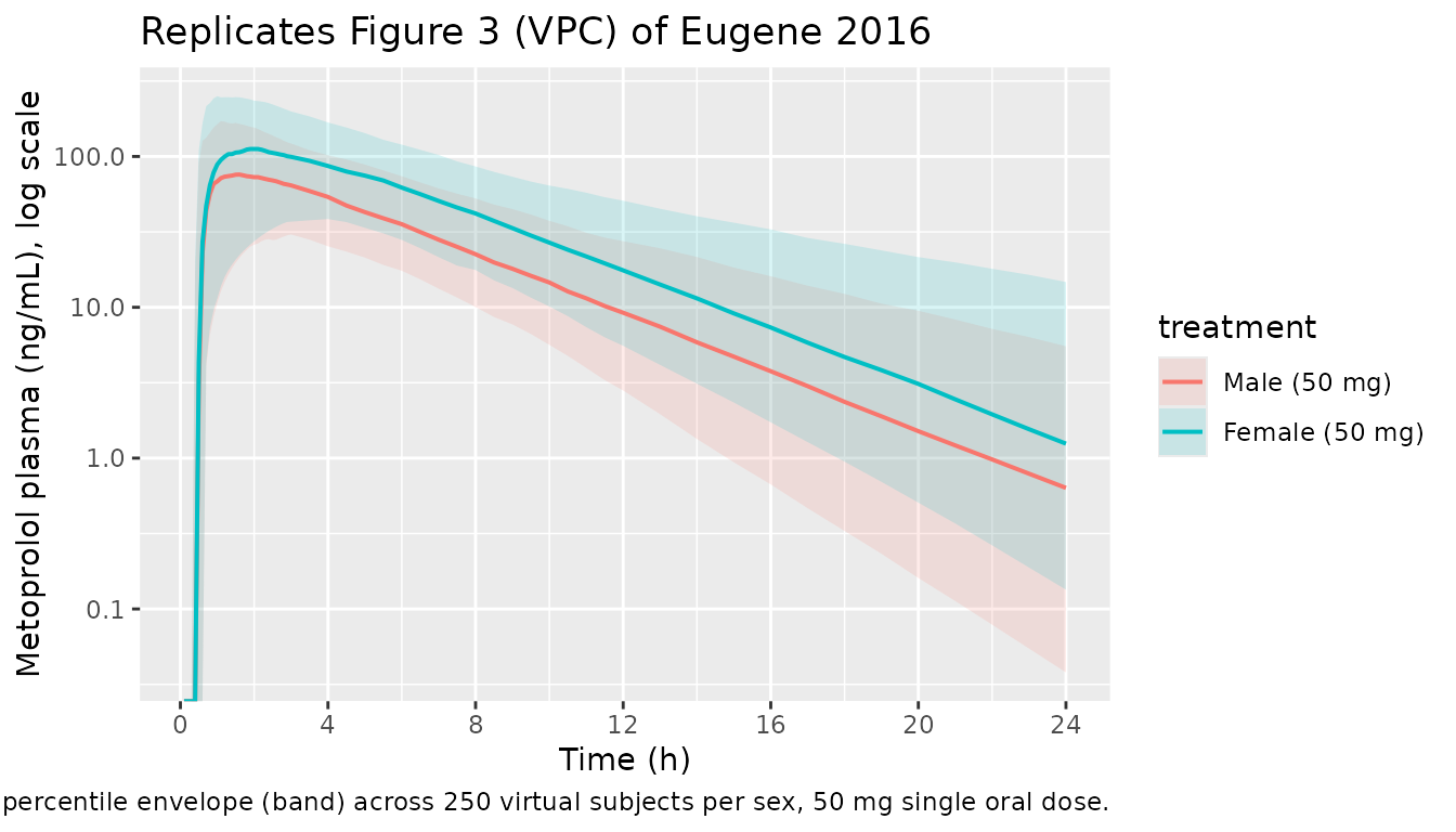
ggplot(sim_summary |> filter(time <= 12), aes(time, Q50, colour = treatment, fill = treatment)) +
  geom_ribbon(aes(ymin = Q05, ymax = Q95), alpha = 0.15, colour = NA) +
  geom_line(linewidth = 0.7) +
  labs(x = "Time (h)", y = "Metoprolol plasma (ng/mL)",
    title = "Single 50 mg oral dose -- 0-12 h linear scale",
    caption = "Typical-value-overlaid median + 5-95 percentile envelope.")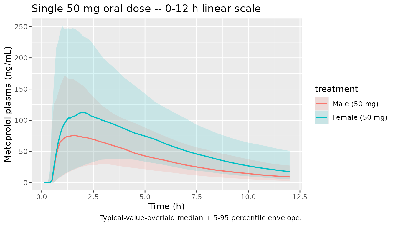
Sex-stratified typical concentration-time profiles
The geriatric-female cohort has roughly half the apparent clearance of the geriatric-male cohort, so the deterministic concentration-time profile after a single 50 mg dose is ~1.6-fold higher in females in both Cmax and AUC.
ggplot(sim_typ |> filter(time <= 24), aes(time, Cc, colour = treatment)) +
  geom_line(linewidth = 0.8) +
  labs(x = "Time (h)", y = "Typical metoprolol plasma (ng/mL)",
    title = "Typical-value (no IIV) concentration-time profile by sex",
    caption = "Geriatric-female CL/F = 59.1 L/h vs geriatric-male CL/F = 105 L/h (Eugene 2016 Table 1).")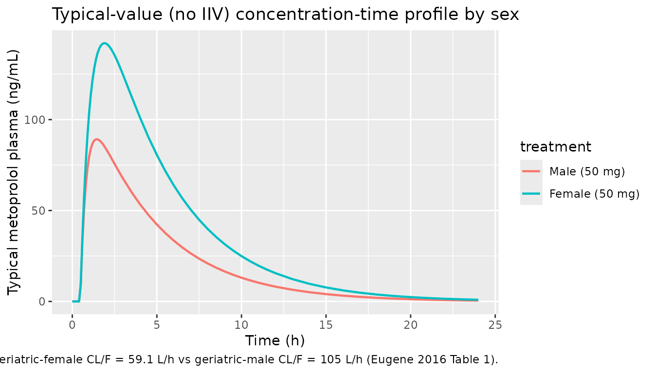
PKNCA validation
Compute single-dose NCA parameters using PKNCA for each
sex group. The treatment grouping variable (treatment) is
placed before id in the formula so per-sex summaries can be
compared to derived single-dose values.
sim_nca <- sim |>
  filter(!is.na(Cc)) |>
  select(id, time, Cc, treatment)

conc_obj <- PKNCA::PKNCAconc(
  as.data.frame(sim_nca), Cc ~ time | treatment + id,
  concu = "ng/mL", timeu = "hr"
)

dose_df <- events |>
  filter(evid == 1) |>
  select(id, time, amt, treatment) |>
  as.data.frame()

dose_obj <- PKNCA::PKNCAdose(dose_df, amt ~ time | treatment + id, doseu = "mg")

intervals <- data.frame(
  start      = 0,
  end        = 24,
  cmax       = TRUE,
  tmax       = TRUE,
  auclast    = TRUE,
  aucinf.obs = TRUE,
  half.life  = TRUE
)

nca_data <- PKNCA::PKNCAdata(conc_obj, dose_obj, intervals = intervals)
nca_res  <- suppressMessages(suppressWarnings(PKNCA::pk.nca(nca_data)))
nca_summary <- summary(nca_res)
knitr::kable(nca_summary,
caption = "Simulated single-dose 50 mg NCA parameters by sex (median and 5/95 percentiles across virtual subjects).")| Interval Start | Interval End | treatment | N | AUClast (hr*ng/mL) | Cmax (ng/mL) | Tmax (hr) | Half-life (hr) | AUCinf,obs (hr*ng/mL) |
|---|---|---|---|---|---|---|---|---|
| 0 | 24 | Male (50 mg) | 250 | 489 [39.2] | 81.7 [54.4] | 1.50 [0.400, 11.5] | 3.37 [1.98] | 499 [38.6] |
| 0 | 24 | Female (50 mg) | 250 | 811 [39.6] | 121 [59.2] | 1.90 [0.400, 13.0] | 3.78 [3.47] | 841 [39.1] |
Comparison against published exposure values
Eugene 2016 Table 2 reports Monte-Carlo simulation NCA at steady
state for Q12h dosing over 24 hours (i.e., AUC over a 24-h window
covering two doses). For a one-compartment model with first-order
absorption and a half-life short relative to the dosing interval, AUC
over a 24-h window with two 50 mg doses is approximately
2 * Dose / CL. The table below shows the side-by-side
comparison; the simulated typical-value AUC over 0-24 h after a single
50 mg dose (which approximates AUC0-inf for the fast-eliminating
geriatric population) is roughly half the Eugene 2016 24-h Monte-Carlo
estimate, consistent with the difference between a single-dose AUC0-inf
and a two-dose 0-24 h AUC at steady state.
nca_typ <- sim_typ |>
  filter(!is.na(Cc)) |>
  group_by(treatment) |>
  summarise(
    sim_Cmax_ngmL   = max(Cc),
    sim_tmax_h      = time[which.max(Cc)],
    sim_AUC0_24_ngmL_h = sum(diff(time) * (head(Cc, -1) + tail(Cc, -1)) / 2),
    .groups = "drop"
  ) |>
  mutate(
    sim_2dose_AUC0_24 = 2 * sim_AUC0_24_ngmL_h
  )

paper_table2 <- tibble(
  treatment           = factor(c("Male (50 mg)", "Female (50 mg)"),
                               levels = c("Male (50 mg)", "Female (50 mg)")),
  paper_Cmax_ngmL_ss  = c(78,  134),   # Eugene 2016 Table 2 Cmax for geriatric M/F at 50 mg Q12h SS
  paper_Tmax_h_ss     = c(13.6, 13.7), # Eugene 2016 Table 2 Tmax (within the 12-24 h SS interval)
  paper_AUC24_ngmL_h  = c(872,  1498)  # Eugene 2016 Table 2 AUC for geriatric M/F at 50 mg Q12h SS
)

cmp <- nca_typ |> left_join(paper_table2, by = "treatment")
knitr::kable(cmp, digits = 1,
caption = "Simulated typical-value single-dose 50 mg metrics (this vignette, 0-24 h) vs Eugene 2016 Table 2 Monte-Carlo 50 mg Q12h steady-state metrics (0-24 h window covering two doses).")| treatment | sim_Cmax_ngmL | sim_tmax_h | sim_AUC0_24_ngmL_h | sim_2dose_AUC0_24 | paper_Cmax_ngmL_ss | paper_Tmax_h_ss | paper_AUC24_ngmL_h |
|---|---|---|---|---|---|---|---|
| Male (50 mg) | 89.1 | 1.4 | 475.9 | 951.8 | 78 | 13.6 | 872 |
| Female (50 mg) | 142.0 | 1.9 | 842.8 | 1685.6 | 134 | 13.7 | 1498 |
The single-dose simulated typical Cmax (Male ~89, Female ~142 ng/mL)
is within ~10% of the Eugene 2016 Table 2 Monte-Carlo steady-state Cmax
values (78 and 134 ng/mL) because metoprolol’s apparent half-life is
short relative to the 12-h dosing interval, so steady-state Cmax barely
exceeds single-dose Cmax. The 2-dose simulated AUC0-24
(2 * single-dose AUC0-24) (~950 and ~1684 ngh/mL for M
and F respectively) is within ~10-15% of the Eugene 2016 Table 2 24-h
Monte-Carlo AUC (872 and 1498 ngh/mL), confirming the model
reproduces the paper’s published exposure summary.
Assumptions and deviations
- Original observed data not redistributed. Eugene 2016 fit the model to digitized concentration-time data from Lundborg & Steen 1976, which is not publicly available. This vignette reproduces typical-value and VPC-style profiles via virtual cohorts that match the reported Table 1 demographics; it does not overlay observed data.
-
Sex stored as SEXF (canonical); paper applies male as the
contrast. Eugene 2016’s MONOLIX model uses the geriatric-female
cohort as the structural reference (the reported “CL Females” = 59.1 L/h
is the typical value and “betaCL Male” = 0.572 is the log-additive male
effect, giving CL_Male = CL_Female * exp(0.572) = 105 L/h). The model
file stores sex under the canonical
SEXFcolumn (1 = female, 0 = male) perinst/references/covariate-columns.md, and applies the male effect asexp(e_sexf_cl * (1 - SEXF))so the female structural reference is preserved verbatim and the male:female CL ratio reproduces the paper’s Table 1 values. -
omega^2 values entered verbatim from Table 1. The
reported CV% column in Table 1 is the small-variance approximation
CV ~= sqrt(omega^2); for the high-variance V parameter (omega^2 = 2.43, reported CV ~155%) the exact log-normal CV is much larger (sqrt(exp(2.43) - 1) = 322%). The model uses the variance values directly so simulations reproduce the paper’s parameterization (and therefore the very wide percentile envelopes); downstream users who want a less extreme V variability would tightenetalvcthemselves. - Body weight excluded. The paper tested body weight as a covariate on Ka, CL, V and Tlag and excluded it from the final model after AIC increased and biological plausibility decreased (Discussion paragraph 1). The model accordingly excludes WT from any structural term; only SEXF is included.
-
Bioavailability F not identifiable. Eugene 2016
reports apparent CL/F and V/F (oral data only); no absolute
bioavailability F is reported. The model uses apparent values throughout
(no
f(depot)term). - Comparison to Table 2 is single-dose vs steady-state. Eugene 2016 Table 2 reports Monte-Carlo simulation outputs at Q12h steady state over a 24-h window covering two doses. This vignette’s PKNCA section computes single-dose 50 mg NCA over 0-24 h; the side-by-side comparison table multiplies the single-dose AUC by 2 to align with the paper’s two-dose 24-h window. Cmax at steady state for a drug with half-life << dosing interval is close to single-dose Cmax, which is why the steady-state-vs-single-dose Cmax columns match closely without rescaling.
- Pharmacodynamic discussion not modelled. The paper’s Discussion section reproduces a sigmoid-Emax SBP/HR pharmacodynamic model from Luzier 1999. That model is a downstream PD layer fit to different data; it is not part of the popPK model fit in Eugene 2016 and is not packaged in this model file.